Computational fluid dynamics-based hull form optimization using approximation method

ABSTRACT

With the rapid development of the computational technology, computational fluid dynamics (CFD) tools have been widely used to evaluate the ship hydrodynamic performances in the hull forms optimization. However, it is very time consuming since a great number of the CFD simulations need to be performed for one single optimization. It is of great importance to find a high-effective method to replace the calculation of the CFD tools. In this study, a CFD-based hull form optimization loop has been developed by integrating an approximate method to optimize hull form for reducing the total resistance in calm water. In order to improve the optimization accuracy of particle swarm optimization (PSO) algorithm, an improved PSO (IPSO) algorithm is presented where the inertia weight coefficient and search method are designed based on random inertia weight and convergence evaluation, respectively. To improve the prediction accuracy of total resistance, a data prediction method based on IPSO-Elman neural network (NN) is proposed. Herein, IPSO algorithm is used to train the weight coefficients and self-feedback gain coefficient of ElmanNN. In order to build IPSO-ElmanNN model, optimal Latin hypercube design (Opt LHD) is used to design the sampling hull forms, and the total resistance (objective function) of these hull forms are calculated by Reynolds averaged Navier–Stokes (RANS) method. For the purpose of this article, this optimization framework has been employed to optimize two ships, namely, the DTMB5512 and WIGLEY III, and these hull forms are changed by arbitrary shape deformation (ASD) technique. The results show that the optimization framework developed in this study can be used to optimize hull forms with significantly reduced computational effort.

KEYWORDS:

• Hull forms optimization
• approximate method
• IPSO-Elman neural network
• optimal Latin hypercube design
• arbitrary shape deformation

1. Introduction

In recent years, hull form optimization has gained great interest for the purpose of minimizing the total resistance which results in minimizing the running cost. At the end of the 1990s, the optimization theory was introduced into the field of hull form design by potential flow theory. Dawson method was used to calculate the sum of flat friction resistance and wave-making resistance which was as the objective function to design the ship-type (Kim, 1995). Wave-making resistance was calculated by potential flow method, and optimal design of hull form was carried out with adjoint optimization method (Huan & Huang, 1998). Rankine source was used to calculate the wave resistance and viscous resistance of Series60, and the hull form with the lowest resistance was obtained by nonlinear programing method (Zhang & Zhang, 2015).

With the rapid development of computational fluid dynamics (CFD) technique and optimization technique, hull forms design based on simulation-based design (SBD) technique has become the main trend in the twenty-first century (Kim & Yang, 2010; Tahara, Peri, Campana, & Stern, 2008). The CFD tools have become the main method for calculating the hull resistance and simulating the flow field, but its calculation time is rather long. In order to promote the application of SBD technique to the practical engineering, and to reduce the computational time of a typical CFD work, the application of approximate technique has become the key to the development in ship-type optimization. By processing of approximate technique, the original complex problem is turned into a relatively small approximate sub-problem, and the optimal solution of the original problem is obtained by successive approximation. The issue of predictions using the approximate model has been highlighted by some designers not only in the engineering (Chang, Feng, Liu, Zhan, & Cheng, 2012; Kamiński, 2015; Qian, Mao, Wang, & Yun, 2012) but also in the real-life (Chau & Wu, 2010; Wang, Kwokwing, Xu, & Chen, 2015; Wu, Chau, & Li, 2009). In recent years, one of the approximate techniques widely used is the neural network, which is a kind of information processing method developed according to the enlightenment of biological nervous system. On account of the computer simulation, it can predict and analysis the data by learning, control and identification. Now, it has been applied into different kinds of optimization problems (Hu & Balakrishnan, 2005; Liu & Luo, 2005; Liu, Tian, Liang, & Li, 2015; Puig, Witczak, Nejjari, Quevedo, & Korbicz, 2007; Zhang, 2016). The ElmanNN is a typical multi-layer dynamic recurrent neural network, and it has a stronger global stability and a characteristic of time-varying since adding the contest nodes to the hidden nodes of feed-forward network as time delay operator (Ding, Jia, Su, Xu, & Zhang, 2008). Besides, ElmanNN has been compared with BPNN which is derived from data prediction (Ding et al., 2008; Zhang, Hao, Kong, & Li, 2013; Zhou, Yang, & Yang, 2011), and they all found that the predicting precision and convergence rate of ElmanNN are much higher than BPNN. Li and Liang (2007) carried out a comparison of ElmanNN and RBFNN for flood freeway speed limitation and assumed that the ElmanNN has stronger adaptation and better generalization ability and can build the approximate model more accurately. On the basis of the local feedback network function, the ElmanNN can process the data more precision for nonlinear problem (Liu et al., 2015), which is of great important for the hull resistance prediction. Up to now, hull resistance has been predicted by using radial basis function (RBF) (Huang, Wang, & Yang, 2015; Huang & Yang, 2016), artificial neural networks (Couser, Mason, Mason, Smith, & Konsky, 2004), Holtrop and Mennen’s method (Ortigosa, López, & García, 2009), genetic neural network (Chen & Ye, 2009), and BP neural network (Hou, Liu, & Liang, 2016). However, there are few literatures have been published for predicting hull resistance using ElmanNN. In the light of these considerations, an ElmanNN has been used into the hull form optimization in this study to approximately calculate the total resistance values.

Particle swarm optimization (PSO), a kind of intelligent optimization algorithm, was developed by Kennedy and Eberhart in 1995 (Kennedy & Eberhart, 1995). It has obtained a lot of interest in diverse optimization problems because of the advantages of fast convergence, easy implementation and simple calculation rules. Although PSO algorithm has become a relative mature method, it is easy to fall into the local optimal solution. Therefore, many researchers have put forward a variety of improvement measures to prove that the new methods are superior to traditional PSO algorithm. The hybridized technique named PSO-GA algorithm was presented by taking the advantages of both PSO and GA algorithm for solving the nonlinear design optimization problems (Garg, 2016; Nik, Nejad, & Zakeri, 2016). The weighted particle for incorporation into the particle swarm optimization, and the enhanced particle swarm optimizer incorporating a weighted particle (EPSOWP) was developed to improve the evolutionary performance for a set of benchmark function (Li, Wang, Hsu, & Chen, 2014). Based on the random linear combination between the local best position and the global best position, the particle swarm without velocity equation (PSWV) algorithm was studied by Tungadio, Jordaan, and Siti (2016). A novel multi-sub-swarm particles warm optimization (MSSPSO) was used to find multi-solutions for multilayer ensemble pruning model by Zhang and Chau (2009). In this model, the MSSPSO algorithm was used to generate a different pruning based on previous oracle output for each layer. A more fast and accurate input variable selection (IVS) algorithm has been developed by Taormina and Chau (2015) integrating binary-coded discrete fully informed particle swarm optimization (BFIPS) and extreme learning machines (ELM). As we all know, the evaluation of the convergence is one of the most important factors for the PSO algorithm. If the convergence is decreased, the convergence rate of this algorithm will be affected heavily (Han, Li, & Wei, 2006). However, the article above did not mention how to evaluate the premature convergence. In this paper, an improved PSO (IPSO) algorithm has been developed by integrating the randomly distributed inertia weight coefficient and the evaluation of premature convergence. The performance of this new method has been evaluated by employing them in the optimization of the four mathematical functions.

Although ElmanNN has some advantages, there also exist some problems in its application. When dealing with high dimensional data, such as ship resistance values, useful information can be overwhelmed by large quantities of redundant data and relevant redundant information may take up much storage space and may consume a lot of calculation time (Ding et al., 2008). It is also easy to fall into local minimum because the gradient descent method is used to train the network parameters. By developing the improved ElmanNN (Shen et al., 2015; Song & Zhao, 2016; Zhou, Ding, & He, 2013), these problems can be overcome effectively. In this article, to improve the accuracy of the resistance prediction using ElmanNN, an effective IPSO algorithm developed is used to optimize the inertia weight coefficients and self-feedback gain coefficient of ElmanNN. Then the performance of the IPSO-ElmanNN method is compared in the prediction of the ship resistance with the original ElmanNN.

The aim of present work is to describe a practical ship hull form optimization loop using the IPSO-ElmanNN method. An arbitrary shape deformation (ASD) technique is used to alter the geometry of hull. Total resistance in calm water is selected as the objective function, and optimization is carried out at design speed. The IPSO-Elman algorithm is proposed to approximately calculate the total resistance, and the hull form is optimized using an IPSO algorithm. Finally, two ships are presented and discussed: namely, the David Taylor Model Basin (DTMB) model5512 (a ship model of the US Navy Combatant) and the WIGLEY III (a mathematical ship form widely used on the international) ships.

2. Optimizers

2.1. Particle swarm optimization (PSO) algorithm

On the D-dimensional space, the i-th particle velocity and position can be written as Vⁱ = (v_i,1v_i,2v_i,3 … v_i,d) and Xⁱ = (x_i,1 x_i,2 x_i,3 … x_i,d) , respectively. pbest is used to denote the local best solution and gbest is used to denote the global optimal solution. In each of iteration, the particle updates itself by tracking pbest and gbest. After finding these two optimal values, the velocity and position of each particle is updated using the following formulas: (1) (2) where ω is the inertia weight coefficient, c₁ and c₂ are the acceleration coefficients with positive values called cognitive and social parameters, respectively. r₁ and r₂ are the random variables between 0 and 1. Generally, the range of the total number of particles N, c₁ and c₂are reported as follows: 20 ≤ N ≤ 40; c₁ + c₂≤ 4 (Azimifar & Payan, 2016).

2.2. Improved particle swarm optimization (IPSO) algorithm

The inertia weight coefficient ω is a parameter to influence the trade-off between global and local searches within the solution domain. In order to improve the precision of the PSO algorithm, the adjustment of ω will become very important. Large ω can avoid getting into local optimal solution, and small one can effectively accelerate convergence speed of iteration. It can be calculated by constant method, linear decrement method, self-adaptation method and so on. In this paper, ω is subject to a random distribution, so that it can overcome the instability caused by the linear decline of the two aspects.

The formula of ω can be written as: (3) (4) where is the mean value of random weight, σ is the variance of random weight. N(0,1) is the random variable of standard normal distribution. is the minimum value of random weight. is the maximum value of random weight. rand (0,1) is the random variable between 0 and 1.

The convergent degree of PSO algorithm can be obtained from (Wang, Ma, Wang, & Wang, 2011): (5) where Δ is the evaluation index of convergent degree, the smaller the Δ is, the better convergent it will be. is the fitness of the optimal particle, is the fitness average which is calculated by the particles with better fitness than (fitness average of the whole particles) which can be got from , is the i-th particle fitness, n is the size of the particle swarm.

The particle tends to premature convergence if Δ is less than threshold and the optimal solution and the expected optimal solution is not obtained. Consider the minimization problem: (6) (7) At this time, partially inactive particles are modified by Gaussian mutation to early jump out of local optimum and quickly find the global optimal solution. The formal can be written as: (8) where θ is the threshold, for i-th particle satisfying the inequality (8), the mutation is carried out with random one-dimensional location: (9) where η is the coefficient of variation, ξ is the random variable in accordance with N(0,1) distribution.

The general flow chart of IPSO algorithm is as follows:

1. Initialize the velocities and positions of a set of particles randomly.

2. Update the velocities and positions of particles according to Equations (1) and (2).

3. Update the inertia weight coefficient ω using Equations (3) and (4).

4. Calculate the fitness f_i.

5. Update the individual extremum pbest and the group extremum gbest.

6. Determine whether the premature convergence is produced by Equations (6) and (7). If the answer is yes, the population needs to mutate by Equations (8) and (9). If not, repeat the steps 2–6 until the stopping criterion is met.

7. Output the global optimal result.

2.3. Verification and validation for the IPSO algorithm

To verify the applicability of the IPSO algorithm, four functions are studied, as shown in Equations (10–13). PSO and IPSO algorithm are used to find the minimum value of four functions respectively. The parameters of two algorithms are shown in Table 1. (10) (11) (12) (13)

Table 1. Parameters.

Method	N	c1	c2	ω			Δd	θ	η
PSO	40	2	2	0.5	–	–	–	–	–
IPSO	40	2	2	–	0.8	0.5	1e^−4	0.2	0.1

After the completion of optimization, the results are tabulated in Table 2. The optimization results of the IPSO algorithm can get the global optimal solution for four functions, while PSO algorithm and IPSO algorithm with self-adaptive weight and experimental design by Li (2012) were trapped in a local optimum. It can be seen that the IPSO algorithm developed in this paper has very high-precision results in the optimization.

Table 2. Optimization results of different algorithms.

	D	Minimum value	PSO	IPSO	IPSO (Li, 2012)
f1(x) (Rosenbrock)	10	0	5.3067	0	4.855
f2(x) (Schaffer)	10	0	0.009716	0	0.0097
f3(x) (Rastrigrin)	10	0	16.9250	0	3.669
f4(x) (Griewank)	10	0	1.0277	0	0.0694

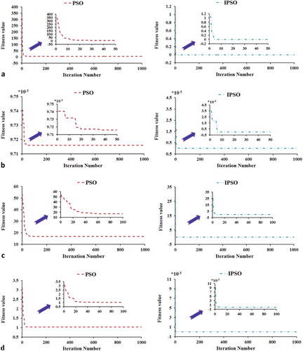
Figure 1 shows a comparison of the iterative processes of the optimization using the PSO and IPSO algorithms individually. As can be seen from the figure, in 1000 iterations, the IPSO algorithm can give a better fitness value which is near to the global optimal solution at the initial stage of optimization compared to the PSO algorithm. Although the mutation operation is added in the IPSO algorithm, the convergence speed of this algorithm is still not affected. The improving of the convergence speed is mainly because the weight coefficient is not a fixed value but a random distribution value. At the early stage of optimization, if the particle is near the global optimum, it can automatically produce a relatively small value to accelerate the convergence speed. If the optimization has got into local extremum at the early stage of optimization, the constantly change of the weight coefficient and the convergence evaluation algorithm can help to overstep the local extremum.

Figure 1. Convergence history of the different algorithms (a) f₁(x), (b) f₂(x), (c) f₃(x), (d) f₄(x).

3. Geometry reconstruction

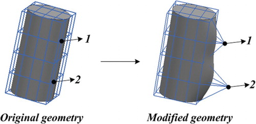
Based on B-spline technique, arbitrary shape deformation (ASD) technique is a method to change the shape of different models by Sculptor tool (Sun, Song, & An, 2010). It requires that the ASD volume is set up outside the body with many control points and connections. When the control points are moved, the shape of the relevant areas can be changed. The new surface can be achieved by the movements of control points, in which the continuity of 3-order can be maintained. This can insure the smoothness of the new model even under the conditions of large deformations. This direct deformation method can make it easy for the change of the complex geometric. Taking a cylinder as an example, the deformation process can be written as follows:

1. Build an ASD volume around the cylinder with many control points and connections between them, as shown in Figure 2. The deformation volume can be finer or coarser, depending on the shape change control desired.

2. Define the control parameters including the position of point and the direction of movement. As can be seen from Figure 2, point 1 and point 2 are taken as control parameters in order to change the geometry shape.

3. Freeze the ASD volume, and change control parameters by the movements of the points according to the requirements of the designers.

4. Get new geometry in term of geometry generation algorithm with modified control points.

Figure 2. Geometry deformation using two parameters.

4. Calculation of total resistance based on CFD

4.1. Mesh generation and boundary conditions

Overset mesh is a method (CD-Adapco, 2014) in which grids are divided for two parts (background grids and overset grids) of the model and then nested into the background grids. The background grids are static and the overset grids can be moved. The flow field information is exchanged at the interface according to the interpolation between each other. Then, the whole flow field can be calculated (Zhao, Gao, & Xia, 2011). In this article, an overset mesh is used to divide the computational domain with linear interpolation, as shown in Figure 3. Figure 3(a) shows the mesh of the whole physical model, and the refined mesh is adopted near the free surface. Figure 3(b) shows the mesh of hull surface.

Figure 3. Grid division of computational domain and hull (a) Mesh of the computational domain, (b) Computational mesh on the ship geometries.

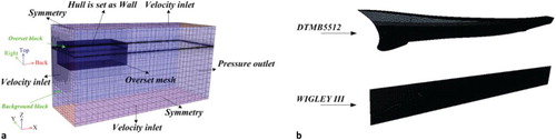
Figure 3(a) also shows the boundary conditions of the computational domain. In the light of the requirement of the overset mesh, the whole model needs two individual blocks which are named as background block and overset block. Background block is only a cuboid, and overset block is a model with Boolean subtraction between the cuboid and the hull. For the background block, the length in front, back, top, bottom and left of the hull are taken as 1.5 L_pp (L_pp is the length between perpendiculars of hull), 6 L_pp, 1 L_pp, 4 L_pp and 3 L_pp, respectively. For the overset block, the length in front, back and left of the hull are taken as 1 L_pp, 1.5 L_pp and 2 L_pp, respectively.

1. Background block: front, top and bottom boundaries are selected as velocity inlet. Back boundary is selected as pressure outlet and both sides of tank are selected as symmetry plane.

2. Overset block: the right side of the cuboid is set as the symmetry plane and the rest of surface is set as overset mesh. A no-slip boundary condition is set for the hull geometry.

4.2. Calculation methods

In this study, Star-CCM+ is used as a RANS solver. Based on the user manual of the software (CD-Adapco, 2014), the hull is set as the fixed model and floating on the water under design draft. The total resistance in calm water is calculated by using RANS equations (Ferziger & Peric, 2002) based on the SIMPLE (Patankar & Spalding, 1972) algorithm. The RNG k-ϵ model (Yakhot & Orszag, 1986) is selected as turbulence model. A Volume of Fluid (VOF) model (Hirt & Nichols, 1981) is selected to model and position the free surface. The whole computational domain is discretized by finite volume method. The second-order upwind difference scheme is adopted for the convection term and the centric difference scheme for the dissipation term. The ship speed is taken as the initial velocity to start the iterative calculation.

5. The establishment of approximation method for CFD data

5.1. Optimal Latin Hypercube Design (Opt LHD)

There are a variety of experimental designs, such as central composite, orthogonal design, full factorial design and so on. Among them, the random Latin hypercube design algorithm is improved to obtain better uniform, space-filling and equilibrium, which is known as optimal Latin hypercube design (Opt LHD) algorithm (Morris & Mitchell, 1995). Matrix generating step is as follows:

m test points, n factors constitute the n*m matrix: (14) Analyze the i-th test point: (15) The Latin hypercube design algorithm is used to generate an initial design matrix according to the formula (15), and then update the design matrix through element exchange. Finally, optimal space filling is obtained by principle of max-min distance: (16) where t = 1 or 2, 1 ≤ i, j ≤ m, i≠j, the sampling point d(x_i,x_j) is the minimum distance between x_i and x_j.

Now take 3 levels of 3 factors as example. The samples distributions are obtained by random Latin hypercube design and optimal Latin hypercube design for nine experiments, as shown in Figure 4. As can be seen from the figure, the samples are more uniform and accurate to express the characteristics of spatial distribution by the optimal Latin hypercube design.

Figure 4. Comparison of samples (a) Random latin hypercube design, (b) Optimal latin hypercube design (above: Present study, below: Wang & Lu, 2015).

Based on the Opt LHD algorithm, 200 schemes are designed to calculate the total resistance, as shown in Table 3. The space distributions of samples are shown in Figure 5. The total resistance R_T is calculated by RANS-CFD method in Section 4. The total resistance coefficient C_T can be obtained using the following equation: (17) where ρ is the fluid density, v_hull is the speed of hull, S is the wetted surface area.

Figure 5. Space distributions of samples (a) DTMB5512, (b) WIGLEYIII.

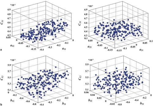
Table 3. Experiment samples.

	DTMB5512					WIGLEY III
No.	a11	a12	a21	a22	CT1*10^−3	b11	b12	b21	b22	CT2*10^−3
1	−0.0201	−0.02442	0.0623	−0.0479	4.341	−0.0369	−0.5494	−0.061	−0.00275	5.536
2	−0.2533	−0.03809	0.0573	−0.0468	4.373	−0.3791	−0.5237	−0.6747	0.04178	5.206
3	−0.1065	−0.09362	−0.1148	0.0884	4.343	−0.0932	−0.7357	−0.0161	0.00361	5.577
4	−0.201	−0.02528	−0.0143	−0.0214	4.342	−0.3068	−0.2731	−0.2924	0.03976	5.369
5	−0.3075	−0.08337	−0.0721	−0.1115	4.472	−0.249	−0.0867	−0.7229	0.04294	5.297
6	−0.2432	−0.01503	−0.145	−0.019	4.341	−0.008	−0.3373	−0.1221	0.036	5.426
7	−0.3176	−0.0808	−0.0759	−0.0329	4.387	−0.3936	−0.3502	−0.1896	0.02993	5.311
8	−0.0422	−0.00392	−0.1136	0.0769	4.352	−0.1044	−0.5783	−0.1542	0.01287	5.502
9	−0.0683	−0.10131	−0.0683	−0.0075	4.497	−0.2506	−0.1382	−0.4305	−0.00969	5.402
10	−0.203	−0.13975	0.0824	0.0561	4.383	−0.3438	−0.045	−0.3181	0.04612	5.536
…	…	…	…	…	…	…	…	…	…	…
…	…	…	…	…	…	…	…	…	…	…
197	−0.2915	−0.12779	−0.057	−0.0098	4.493	−0.355	−0.4016	−0.7454	0.02212	5.211
198	−0.3437	−0.06286	0.0673	0.0792	4.361	−0.3213	−0.0257	−0.2024	0.01402	5.291
199	−0.3276	−0.07739	0.0523	0.0098	4.362	−0.1141	−0.3181	−0.6008	0.05913	5.358
200	−0.2854	−0.10387	−0.0043	0.033	4.451	−0.0273	−0.498	−0.3566	0.00448	5.502

In the Table 3: a₁₁, a₁₂, a₂₁, and a₂₂ are the design variables of the DTMB5512 ship, which have been listed in Section 6. C_T1 is the total resistance coefficient of the DTMB5512 ship. b₁₁, b₁₂, b₂₁, and b₂₂ are the design variables of the WIGLEY III ship, which have been listed in Section 6. C_T2 is the total resistance coefficient of WIGLEY III ship.

5.2. Elman neural network

The ElmanNN was proposed by Elman in 1990 (Elman, 1990). Its main structure is feed forward connection, which includes the input nodes, hidden nodes, context nodes and output nodes, as shown in Figure 6. The input nodes, hidden nodes and output nodes are similar to the feed forward neural network. The input nodes unit only plays the role of signal transmission, and output nodes unit plays the role of the linear weighting. The context nodes are used to memory the previous output value of the hidden nodes and then return to the input.

Figure 6. The framework of ElmanNN (above: Present study, below: Wang et al., 2011).

Nonlinear state space equations of ElmanNN can be written as: (18) (19) (20) where w³ represents the connection weight from the hidden nodes to the output nodes, x(k) means the output of the hidden nodes. w¹ represents the connection weight from the context nodes to the hidden nodes, w² represents the connection weight from the input nodes to the hidden nodes. x_c(k) means the output of the context nodes. β is the self-feedback gain coefficient. g(*) represents the transfer function of the output nodes, f(*) represents the transfer function of the hidden nodes.

The error function can be written as: (21) The dynamic learning algorithm can be summarized as follows: (22) (23) (24) where , and are the learning step. (25) (26) (27)

5.3. IPSO-Elman neural network

The IPSO-ElmanNN can be expressed as follows:

1. First, the samples are trained according to the input and output. Secondly, the note numbers of the input nodes, hidden nodes and output nodes are designed. Finally, the topology structure of ElmanNN is defined.

2. Define the parameters of IPSO algorithm, which includes the population size, number of iterations, inertia factor and acceleration coefficients.

3. Define the evaluation function of particles. The mean square error function G is used as the fitness evaluation function of the particles. The position of the particle with the lowest fitness is the optimal solution of the model when the iteration is stopped. The fitness function can be defined by the following equation: (28) where y_i(Elman) is the i-th predicted value by ElmanNN, y_i(CFD) is the i-th expected output by CFD method.

4. The velocities and positions of a set of particles are initialized randomly.

5. Update the velocities and positions of particles and inertia weight coefficient ω.

6. Calculate the fitness using the formula (28).

7. Update the individual extremum pbest and the group extremum gbest according to the fitness of the particles.

8. Update the solution, and adjust the weights w¹, w², w³, and self-feedback gain coefficient β.

9. Evaluate whether the premature convergence is produced. If the answer is yes, mutate the population. If not, repeat the steps 5–9 until the final end is met.

10. The optimal result is used to train the weights and self-feedback gain coefficient, and then output prediction results of hull resistance.

5.4. Verification and validation for IPSO-ElmanNN

In order to test the effect of the IPSO-ElmanNN, ElmanNN and IPSO-ElmanNN prediction models are implemented in MATLAB (R2016a) with the samples from Table 3. Two algorithms are then used to predict the total resistance subsequently. The cell numbers of input nodes, hidden nodes and output nodes are 4, 12 and 1, respectively. Figures 7 and 8 show the predictions results of the total resistance coefficients for two ships in question. α is the deviation between the ElmanNN//IPSO-ElmanNN and the CFD methods. Table 4 shows the average error results of these predictions.

Figure 7. Prediction results of C_T1 for DTMB5512ship (a) The prediction of the C_T1using ElmanNN, (b) The prediction of the C_T1using IPSO-ElmanNN.

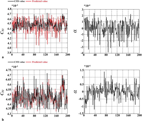
Figure 8. Prediction results of C_T2 for WIGLEYIIIship (a) The prediction of the C_T2using ElmanNN, (b) The prediction of the C_T2using IPSO-ElmanNN.

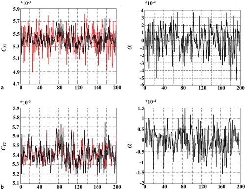
Table 4. Result of the total resistance coefficient prediction based on the different algorithms.

	Average Error (%) for 200 sampling hull forms
Training algorithms	DTMB5512	WIGLEY III
ElmanNN	8.89*10^−5	1.41*10^−4
IPSO-ElmanNN	3.2*10^−5	4.7*10^−5

When comparing the IPSO-ElmanNN with the ElmanNN for predicting the total resistance coefficients, the former has improved the prediction accuracy, not only for the DTMB5512 (with the average error about 3.2*10⁻⁵%), but also for the WIGLEY III (with the average error about 4.7*10⁻⁵%). The reason of this improved performance is that the IPSO algorithm has found a set of more suitable coefficients to train the ElmanNN in order to avoid the difficulty in choosing the coefficients through experience. Although the forecasting precision of the IPSO-Elman algorithm is preferable to the Elman algorithm, there are some errors between the CFD data and prediction data. The main reason for such errors is that the number of samples is not adequate. The network training results can be improved effectively by increasing the number of training samples.

6. Hull form optimization problems

6.1. Optimize processes

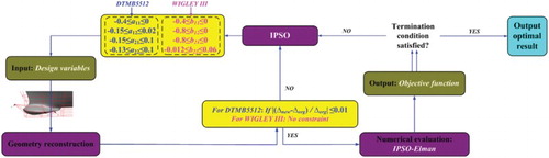
In this paper, optimization process is shown in Figure 9, including the following five steps:

1. Change design variables using the IPSO algorithm.

2. On the basis of a set of design variables, change hull form shape using the ASD technique.

3. Calculate the displacement of each new hull and compare with the constraint. If the condition is met, continue to calculate, otherwise return to step 1 to recalculate the new hull.

4. Calculate the total resistance in calm water using IPSO-ElmanNN, and then save the result.

5. Repeat steps 1–4 until the stopping criterion is met. Then the new hull can be output. The whole work is completed on the ISIGHT platform (Wang, Mo, & Zhang, 2011).

Figure 9. Flow chart of the optimization loop.

6.2. Geometry

In this paper, the DTMB5512 and WIGLEY III ships are selected as optimization models. The modified area have been shown in Figure 10. The major characteristics are shown in Table 5.

Figure 10. Modified region of hull forms.

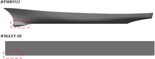
Table 5. Major characteristics of two ships.

Hull forms	DTMB5512	WIGLEY III
Design speed Fr	0.28	0.3
Length between perpendiculars Lpp(m)	3.048	3
Draft d (m)	0.132	0.1875
Breath B (m)	0.409	0.3
Displacement Δ (kg)	86.4	78
Block Coefficient CB	0.507	0.4622

6.3. Optimization strategy

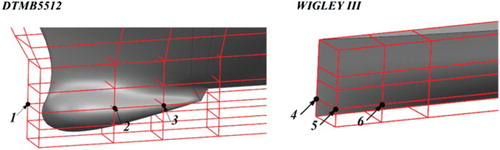
The objective function is the total resistance coefficients C_T1 (DTMB5512) and C_T2 (WIGLEY III) in calm water at design speed. The displacement constraint has been defined in formula (29) (only for DTMB5512). The design variables, a₁₁, a₁₂, a₂₁ and a₂₂ (DTMB5512) and b₁₁, b₁₂, b₂₁ and b₂₂(WIGLEY III) have been shown in Table 6. (29) where _new represents the variable of new hull, and _org represents the variable of parent hull.

Table 6. Control parameters of two ships.

Hull forms	Design variables	No.	Moving directions	Constraints
DTMB5512	a11	1	X	−0.4 ≤ a11 ≤ 0
	a12	1	Z	−0.15 ≤ a12 ≤ 0.02
	a21	2	Y	−0.15 ≤ a21 ≤ 0.1
	a22	3	Y	−0.13 ≤ a22 ≤ 0.1
WIGLEY III	b11	4	X	−0.4 ≤ b11 ≤ 0
	b12	5	Y	−0.8 ≤ b12 ≤ 0
	b21	6	Y	−0.8 ≤ b21 ≤ 0
	b22	4	Z	−0.012 ≤ b22 ≤ 0.06

In the Table 6: No.1 to No.6 are the positions of design variables, as shown in Figure 11.

Figure 11. Control positions of two ships.

6.4. Results and discussion

Since the calculation of the total resistance costs less than two minute under the help of the IPSO-ElmanNN, the optimization efficiency has been greatly improved compared with CFD runs optimization loop. After the completion of the optimization, the excellent hull forms with lower total resistance are obtained. The work is carried out on the Intel Corei5-5200U CPU @2.2 GHz, and the CFD runs in this paper are using the ARCHIE-WeSt Height Performance Computer (http://www.archie-west.ac.uk). Table 7 shows the comparison of the obtained optimization results. The results clearly state that the total resistance of the optimized hull-A is decreased by 5.58%, and the optimized hull-B is decreased by 5.19%. Following this, further calculations are carried out for other speeds and comparison is made against the parent hull by RANS-CFD results and the EFD data obtained from Iowa Institute of Hydraulic Research (Gui, Longo, & Stern, 2001a,2001b; Longo & Stern, 2005) and Delft University of Technology (1992), as shown in Figure 12. For the optimized hull-A, C_T1 decreases at all speeds especially in design speed and high speed, and for the optimized hull-B, C_T2 decreases at all speeds especially in the design speed.

Figure 12. The total resistance coefficients for a range of Fr numbers (a) DTMB5512, (b) WIGLEYIII.

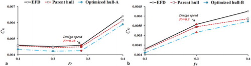
Table 7. Resistance results of the optimized hulls.

Method	Parent hulls	Optimized hulls	Fr	CTorg/CTopt
IPSO-ElmanNN + IPSO	DTMB5512	Optimized hull-A	0.28	1.0591
	WIGLEY III	Optimized hull-B	0.3	1.05468

Figure 13 shows the comparison of the hull lines for parent hull and optimized hulls. Figure 14 shows the comparison of longitudinal wave cut for parent hull and optimized hulls along the y/L_pp = 0.082 plan (z represents the height of free surface). It can be found that the amplitude of waves has been reduced which indicates the reduction in total resistance for the optimized hulls.

Figure 13. Comparison of hull lines (a) DTMB5512, (b) WIGLEYIII.

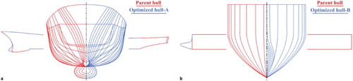
Figure 14. Comparison of wave profile at y/L_pp = 0.082 (a) DTMB5512, (b) WIGLEYIII.

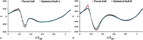
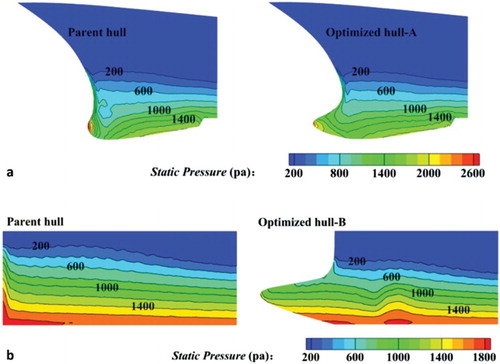
Figure 15 presents the wave patterns for the parent hull and the optimized hulls. As the change of the bow shape for both of the ships, the wave patterns in the forward shoulder have been reduced significant, while the change of the shoulder waves and the stern waves are not very significant. Figure 16 is the comparison of the static pressure on hull surface. The new hull forms have changed the pressure distribution near the bow, and wave-resistance has been decreased which ends the decrease of the total resistance.

Figure 15. Comparison of the wave patterns around the vessels (a) DTMB5512, (b) WIGLEYIII.

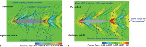
Figure 16. Comparison of the static pressure on the ship surfaces (a) DTMB5512, (b) WIGLEYIII.

7. Conclusion

1. In order to overcome the shortcomings of the PSO algorithm, an IPSO algorithm has been proposed with random weighting method and the evaluation of convergence. Through the test of four mathematical functions, it can be concluded that IPSO algorithm developed in this paper can effectively improve the optimization accuracy.

2. ElmanNN parameters are trained by IPSO algorithm, and IPSO-ElmanNN prediction model is proposed. Then ElmanNN and IPSO-ElmanNN are carried out on the prediction of the hull resistance. The results indicate that the IPSO-ElmanNN has the advantages of precision and stability.

3. Aiming to deal with the challenge of larger surface variation, the ASD technique is used to change the shape of geometry. The new model can be quickly obtained while ensuring the smoothness of surfaces. Because of less design variables, it also can improve the efficiency of ship-type optimization.

4. In terms of hull form optimization problem, IPSO-ElmanNN-based approximate optimization approach is developed and then two ships have been applied in this loop. It is concluded that the approximate optimization system is feasible and rational for optimization of hull forms which can provide relevant technical support in ship-type design.

5. Since the optimization loop in this paper is developed for single objective function (minimum total resistance in calm water), and the seakeeping performances are not taken into account. To obtain a hull form with a better performance, future work will force on the multi-objective optimization including rapidity, seakeeping and manipulation.

Disclosure statement

No potential conflict of interest was reported by the authors.

ORCID

Shenglong Zhang http://orcid.org/0000-0002-9348-4395

Tahsin Tezdogan http://orcid.org/0000-0002-7032-3038

Additional information

Funding

The study in this paper was supported by the grants of the National Science Foundation of China, (No. 51009087) and the grants from the National Science Foundation of Shanghai (No.14ZR1419500). Results were obtained using the EPSRC funded ARCHIE-WeSt High Performance Computer (www.archie-west.ac.uk). EPSRC grant no. EP/K000586/1.