Shape optimization of a feedback-channel fluidic oscillator

ABSTRACT

In this study, a fluidic oscillator was optimized based on the three-dimensional unsteady Reynolds-averaged Navier-Stokes analysis to enhance peak jet velocity at the outlet and simultaneously reduce pressure drop. A multi-objective genetic algorithm performed the optimization with surrogate modeling. The ratios of the inlet nozzle width and the distance between the splitters to the throat width were chosen as the design variables. And, two objective functions related to peak jet velocity at the outlet and pressure drop through the fluidic oscillator were selected for the optimization. Ten design points were selected in the design space using a Latin hypercube sampling method; the objective functions were calculated by unsteady Reynolds-averaged Navier-Stokes analysis at these design points to construct surrogate models that were used to approximate the objective functions. Two different surrogate models, namely response surface approximation and Kriging models were tested. Pareto-optimal front representing a compromise between the two objective functions was obtained from the multi-objective optimization. The optimization results indicated that a jet velocity-oriented optimum design increased the peak jet velocity ratio at the outlet and the friction factor by 11.18% and 16.82%, respectively, when compared to those of a friction factor-oriented design.

KEYWORDS:

• Fluidic oscillator
• multi-objective optimization
• unsteady Reynolds-averaged Navier-Stokes equations
• response surface approximation
• Kriging
• Pareto-optimal solutions

1. Introduction

Any viscous flow subjected to an adverse pressure gradient is prone to separation from a wall. The separated flow on a fluid machinery blade or aircraft wing has an undesirable effect on the aerodynamic performance of the entire system. Separation control using fluidic oscillators is a fast growing state of the art technology. In separation control, a fluidic oscillator injects high momentum fluid into the boundary layer. A jet ejected from the fluidic oscillator entrains high momentum fluid and energizes the boundary layer. Additionally, the pulsing jet increases the mixing rate across the flow field and thereby enhances momentum transfer. In this manner, the pulsing jet ejected from the fluidic oscillator allows viscous fluid to overcome a strong adverse pressure gradient and thus controls the flow separation.

The first fluidic oscillator with feedback loop channels was invented by Warren (1960). The fluidic oscillator again attracted research attention in the past decade and was applied to various processes such as fluid mixing in channels (Joen et al., 2005) and separation control (Burns, 2015; Cerretelli, Wuerz, & Gharaibah, 2010; Lee, Chung, Cho, & Shon, 2007; Nagib, Kiedaisch, Reinhard, & Demanett, 2006; Seele, Graff, Lin, & Wygnanski, 2013; Woszidlo & Wygnanski, 2011; You & Moin, 2008).

A few previous studies examined the effects of fluidic oscillators on airfoil flow characteristics. Woszidlo and Wygnanski (2011) performed an experimental study to evaluate the lift coefficient of an airfoil where an array of fluidic oscillators was embedded at a 60% chord length from the leading edge. The study indicated that the lift coefficients increased from 1.3 to 2.1 owing to the fluidic oscillator array. Lee et al. (2007) experimentally investigated the flow control on an elliptic airfoil using steady blowing and oscillating jets. The results of the study suggested that an oscillating jet at the leading edge was more effective in controlling the flow separation than a steady, blowing jet. Nagib et al. (2006) experimentally evaluated the lift coefficient of an airfoil in various operation conditions, such as mass flow rate, jet velocity ratio, and momentum coefficient, of fluidic oscillators. The results showed that jet velocity ratio was the best performance parameter for separation control. Cerretelli et al. (2010) experimentally investigated fluidic oscillators embedded on wind turbine blades. They reported that the relative lift increased from 10% to 60% and that the stall margin was extended by the fluidic oscillators. You and Moin (2008) numerically investigated the effectiveness of oscillating jets for separation control over an NACA 0015 airfoil. The results indicated good agreements (both qualitatively and quantitatively) with experimental data for both uncontrolled and controlled cases. The study proved that oscillating jets effectively delayed flow separation and increased the lift coefficient by 70% to modify the boundary layer on the airfoil. Seele et al. (2013) experimentally investigated the effects of fluidic oscillator location and distribution on the performance of the vertical tail of an airplane. The results suggested that distributing fluidic oscillators evenly on the surface was considerably more effective in enhancing the performance than concentrating the fluidic oscillators in a specific region. Burns (2015) numerically investigated a novel method to reduce tip leakage flow by sealing the tip clearance of turbine blades with oscillating jets injected from the surface of the rotor tip.

Several numerical and experimental studies were conducted to examine the effects of fluidic oscillator shapes on performance and flow characteristics. Yang, Chen, Tsai, Lin, and Sheen (2007) experimentally tested a fluidic oscillator with step-shaped chamber walls. The results indicated that step-shaped walls promoted conditions to initiate oscillation and caused recirculation vortices to be more stable. Ostermann, Woszidlo, Nayeri, and Paschereit (2015) performed a comparative study on the pressure drop and jet deflection between angled and curved fluidic oscillators. The findings revealed that the curved fluidic oscillator generated less of a pressure drop and a larger jet deflection. Kim, Moin, and Seifert (2015) numerically evaluated the frequency and maximum jet velocity of a novel fluidic oscillator. The results showed that the Strouhal number was constant, and the maximum jet velocity increased as inlet pressure increased. A fluidic oscillator incorporated with a stationary rotating vortex inside a chamber was devised and experimentally examined by Tesar (2015). The findings suggested that this type of fluidic oscillator generated oscillation frequencies of up to 8.2 kHz. Xu and Meng (2013) performed an experiment to investigate the effect of fluidic oscillator configuration on the oscillation frequency. The results indicated that the frequency was dependent on the exit nozzle width, feedback channel width, and chamber shape.

Recent studies used optimization techniques based on the analysis using three-dimensional (3D) Reynolds-averaged Navier-Stokes (RANS) equations to design better systems with lower computational cost for various thermo-fluid engineering applications (Kim & Kim, 2006; Kim & Lee, 2007; Lee & Kim, 2015). In most engineering designs, multi-objective optimization is required owing to multiple disciplines and objectives. Recently, the surrogate modeling of objective functions has become a popular method to reduce the computing time required for repeated evaluations of objective functions (Queipo et al., 2005). Papila, Shyy, Griffin, and Dorney (2011) compared two surrogate models, namely the response surface approximation (RSA) model (Myers, Montgomery, & Anderson-Cook, 2016) and radial basis neural networks model in the optimization of supersonic turbines. Husain, Lee, and Kim (2011) conducted the multi-objective optimization of a dimple channel using two surrogates, i.e. RSA and Kriging (KRG) models. Gao, Wang, Pang, and Cao (2016) performed a shape optimization of autonomous underwater vehicle (AUV) hulls. This optimization proved that the traditional AUV hull shape is not good for drag reduction. In order to maximize the performance of a bidirectional impulse turbine, shape optimization based on surrogate models was performed by Ezhilsabareesh, Rhee, and Samad (2017). Both the shaft power and pressure drop across the turbine were considered as objective functions. Through the optimization, the turbine efficiency was increased by 10.4%. Recently, there have been several other researches about real-life applications of contemporary soft computing techniques in different fields (Taormina & Chau, 2015; Wang, Chau, Xu, & Chen, 2015; Zhang & Chau, 2009).

Although some investigations examined the effects of fluidic oscillator shape on performance, systematic optimization of fluidic oscillators was not found in the literature. Hence, the present study investigated the multi-objective optimization of a fluidic oscillator using a multi-objective genetic algorithm (MOGA) and 3D unsteady RANS analysis to simultaneously enhance peak jet velocity at the outlet and reduce pressure drop. Optimization of a fluidic oscillator with multiple design variables generally requires a huge number of 3D unsteady RANS analyses of objective functions, which is a time-consuming job. However, in this work, the computational time was greatly reduced by employing surrogate modeling of objective functions. Two different surrogate models, RSA and KRG models, were tested to approximate the objective functions. The objective functions were calculated by unsteady RANS analysis at 10 design points to construct the surrogate models.

2. Fluidic oscillator model

A feedback-channel fluidic oscillator is one of the general types of fluidic oscillators that has two feedback channels connecting the upstream and downstream of a chamber as shown in Figure 1. The fluid flows steadily through the inlet nozzle owing to a pressure source. A jet formed upstream of the chamber attaches to one of the chamber walls because of the Coanda effect (Panitz & Wasan, 1972). The Coanda effect is the tendency of a jet to remain attached to a solid surface. Downstream of the chamber, a splitter divides the jet into a feedback channel and the outlet nozzle. The feedback channel flow then returns upstream of the chamber and pushes the jet to the opposite wall of the chamber. Following this, an oscillating jet is ejected from the outlet nozzle. The same process is repeated to complete the oscillation cycle. This mechanism allows the fluidic oscillator to generate a self-induced and self-sustained oscillating jet without any moving parts.

Figure 1. A schematic of the fluidic oscillator and computational domain.

The present study employed a feedback-channel fluidic oscillator that was experimentally investigated by Yang et al. (2007). The study reported that the Coanda effect occurred in an inlet flow rate ranging from 7 L/min to 75 L/min; the frequency of flow oscillation linearly increased with the inlet flow rate while the Strouhal number was nearly constant at 0.0025 in the inlet flow rate ranging from 7 L/min to 75 L/min. Therefore, 25 L/min was selected as the inlet flow rate in the present study where the fluidic oscillator was numerically investigated and optimized.

Figure 2 indicates the geometrical parameters of the fluidic oscillator. The throat width (d_th), hydraulic diameter of the throat (D_h), feedback channel width (b), and fluidic oscillator depth (H) correspond to 5.2 mm, 9.4 mm, 3 mm, and 40 mm, respectively.

Figure 2. Geometric parameters.

3. Numerical analysis

Figure 1 shows the schematic of the fluidic oscillator and computational domain considered in the present study. The computational domain is symmetric about the y-axis and consists of an inlet nozzle, a chamber, a splitter, a feedback channel, a throat, and an outlet nozzle.

The analysis involved the use of a commercial computational fluid dynamics (CFD) code, ANSYS CFX-15.0® (2013), to solve the continuity and RANS equations for a 3D unsteady, incompressible flow in the fluidic oscillator. Numerical schemes of second-order accuracy were used to discretize the convection terms of the governing equations. The k-ε model was used as the turbulence closure model. Vasta, Koklu, Wygnanski, and Fares (2012) also used the k-ε model in a numerical investigation of a fluidic oscillator that had geometry similar to the model considered in the present study; their findings indicated that the numerical results for mean and standard deviations of jet velocity profile agreed well with experimental data. In the present study, unstructured tetrahedral meshes were generated in most of the computational domain, and prism meshes were generated near the walls by the pre-processing software (ANSYS ICEM-CFD®). The first grid points adjacent to the wall were placed at y⁺ > 30 to implement empirical wall functions.

The working fluid was water. The Reynolds number based on the hydraulic diameter of the throat and a reference velocity (U_ref = 1.57 m/s) corresponded to 14,570. A uniform velocity was assumed at the inlet of the inlet nozzle. A constant pressure was assigned at the outlet of the fluidic oscillator. A no-slip boundary condition was adopted on all the walls.

The time step was set as 0.001 s to adjust a Courant number less than 10. The root-mean-square relative residual values were kept below 1.0 × 10⁻⁴ as a convergence criterion. A personal computer with an Intel Core i7 2.67 GHz CPU was used for the computations; the total computational time to obtain a single converged solution was in a range of 7 to 8 days with approximately 10 iterations for each time step.

4. Optimization methods

Figure 3 illustrates the optimization procedure employed in the study. Design variables, design space, and objective functions were determined to define the optimization problem in the first step. A design-of-experiment (DOE) technique was used to select the design points in the design space. The values of the objective function were calculated based on unsteady RANS analysis at the design points. These values were used to construct surrogate models of the objective functions. The Pareto-optimal solutions were determined using the MOGA. The optimization steps are explained in detail in the following sub-sections.

Figure 3. Optimization procedure.

4.1. Design variables and objective function

A previous study investigated the effects of the fluidic oscillator geometry on the velocity ratio and pressure drop (Jeong & Kim, 2016). The aforementioned study reported that the maximum F_VR and F_f were commonly found at w/d_h = 0.19, which corresponded to the lower limit of the tested range. Additionally, F_VR and F_f decreased with increase in w/d_h. This indicates that the two objective functions presented a trade-off. Trends of variations in the objectives with d_s/d_h were similar to those with w/d_h. The maximum F_VR and F_f were commonly found at d_s/d_h = 0.53, which also corresponded to the lower limit of the tested range, and the two objective functions decreased as d_s/d_h increased. Conversely, the two objective functions were not sensitive to the other three design variables, i.e. outlet nozzle width, feedback channel width, and chamber length. Based on these results, ratios of the inlet nozzle width (w/d_h) and the distance between the splitters (d_s/d_h) to the throat width were determined as the design variables for optimization (as shown in Figure 2). The design space was determined as shown in Table 1.

Table 1. Design space.

Design variable	Lower limit	Reference	Upper limit
w/dth	0.19	0.37	0.94
ds/dth	0.53	1.45	2.34

In the present study, two objective functions related to the peak jet velocity at the exit and pressure drop through the fluidic oscillator were selected for the optimization. The velocity ratio (F_VR) was the first objective function responsible for the enhancement of the peak velocity of the expelled jet at the exit of the oscillator, and it is defined as follows (Greenblatt & Wygnanski, 2000): (1) where Here, U_peak is the peak jet velocity at the exit of the oscillator during the oscillation period, and U_ref is the reference velocity that is defined by considering the continuity equation (Ostermann et al., 2015). Additionally, denotes the mass flow rate, A_ref denotes cross-sectional area of the throat, and ρ denotes the density of the working fluid. The negative sign was considered to minimize the objective function. In separation control applications, the velocity ratio is generally used as a performance parameter for fluidic oscillators.

The pressure drop directly affects the pumping power required to drive the fluid flow through the fluidic oscillator. The objective function related to pressure drop is formulated as follows: (2) where Δp is the pressure drop, D_h is the hydraulic diameter of the throat, and S denotes the distance from the inlet to outlet of the oscillator. The optimization problem was defined as the minimization of both objective functions.

4.2. Design of experiment

Latin hypercube sampling (LHS) (McKay, Beckman, & Conover, 2000; Sack, Welch, Mitchell, & Wynn, 1989) was used for the DOE. Specifically, the LHS discretizes the design space constrained by the upper and lower bounds of the design variables to construct the surrogate models. Hence, LHS is a rational sampling method to find samples with an m × n matrix. Here, m indicates the number of sample points, and n indicates the number of variables. Each of the n columns containing levels 1, 2, … , m were randomly coupled to build a Latin hypercube. The sample points generated through this approach ensured that the entire portion of the design space was represented. In the present work, 10 design points were selected by employing the MATLAB function, lhsdesign.

4.3. Response surface approximation model

The RSA model (Goel et al., 2007) is a methodology to fit a function for discrete responses obtained from numerical analysis. It corresponds to the association between design variables and response functions. The present RSA model adopted the following second-order polynomial: (3) where N indicates the number of variables, β_j and β_ij are unknown coefficients, and x_j denotes variables in the polynomial. The number of coefficients corresponded to (N + 1) × (N + 2)/2 for the second-order polynomial model. The second-order polynomial response functions formulated in Eq. (3) were constructed for F_VR and F_f.

4.4. Kriging model

The KRG model (Martin & Simpson, 2005), can be formulated as a combination of two parts, namely the global model and a systematic departure, as follows: (4) where F(x) denotes the unknown function that is estimated for an unknown dataset. Additionally, f(x) indicates a regression function which represents the known values of the objective function at design points, and it is referred to as the global (trend) model. The second component Z(x) is a systematic departure and generates a localized deviation to interpolate the selected data points. The trend model (denoted as f(x)) and the systematic departure (denoted as Z(x)) were employed to capture large-scale and small-scale variations, respectively.

The KRG model has some options in selecting parameters, i.e. the regression function coefficient, process variance, and spatial correlation function (SCF). Martin and Simpson (2005) tested Maximum Likelihood Estimation (MLE) and Cross Validation (CV) to find optimum values of these parameters and estimated the accuracy of the KRG models. They found that MLE was the better method than CV. Based on this result, the authors used the MLE method to select the parameters in the present work. The KRG model construction with the MLE method was performed using MATLAB. The details of the mathematical formulation for MLE were reported by Martin and Simpson (2005).

4.5. Multi-objectives genetic algorithm

An MOGA (Deb, Pratap, Agarwal, & Metarivan, 2002) was employed to find Pareto-optimal solutions for the optimization problem in the present study. A MATLAB function (gamultiobj) was used to adapt this algorithm. The MOGA explored Pareto-optimal solutions in the reasonable solution space limited by the lower and upper bounds of the design variables. An operator for tournament selection having a size of two was employed for determination of parents for the succeeding generation. The crossover imitated mating in biological populations and paired two units as parents to generate a new unit as a child. The crossover function was set as intermediate, and this generated a new unit by using a weighted-average of the parents. Values of the parameters were set to execute the MOGA as follows: population size = 200, generations = 400, Pareto-front population fraction = 0.7, crossover fraction = 0.8, and function tolerance = 10⁻⁴.

5. Results and discussion

To secure grid dependency and accuracy in the prediction a grid-dependency test and turbulence model test using experimental data were performed in previous work (Jeong & Kim, 2016). The grid-dependency test was performed for the frequency of flow oscillation at the feedback channel of the reference oscillator (w/d_th = 0.37 and d_s/d_th = 1.45), as shown in Figure 4. Four different numbers of grid nodes ranging from 300,000 to 3,400,000 were tested. The results indicated that the optimal number of grid nodes was approximately 2,600,000. In the present study, this grid system was employed to perform a validation of the unsteady RANS analysis for the frequency compared with the experimental results that were obtained by Yang et al. (2007) in a flow rate range from 10 to 65 L/min, as shown in Figure 5. Three different turbulence models, namely shear stress transport (SST), k-ε, and baseline (BSL) (Menter, 1993) models, were used in this validation. As shown in Figure 5, the results with the k-ε model represent the best agreement with the experimental data compared to the other tested turbulence models.

Figure 4. Grid dependency test for frequency of flow oscillations at the feedback channel of the reference fluidic oscillator (Jeong & Kim, 2016).

Figure 5. Validation of numerical results with three turbulence models using experimental data for the frequency of flow oscillation (Jeong & Kim, 2016).

Numerical optimization of the fluidic oscillator was conducted to minimize the two objective functions, F_VR and F_f, using the two design variables, w/d_h and d_s/d_h, respectively. The values of the objective functions were evaluated using a 3D unsteady RANS analysis at the 10 design points selected by LHS. Table 2 lists the values of design variables and objective functions at these design points. Based on these objective function values, RSA and KRG models were constructed for the objective functions (F_VR and F_f) and used as the input functions of the MOGA. Furthermore, R²_adj was used to evaluate the accuracy of the RSA models. It is necessary that must be close to 1 to obtain a good fit. The values for the constructed RSA models of the F_VR and F_f corresponded to 0.9979 and 0.9747, respectively; this indicated that the RSA models were well-fitted (Sack et al., 1989). The constructed RSA models for F_VR and F_f correspond to the following second-order polynomial expressions: (5) (6)

Table 2. Design variables and objective function values at all the LHS design points.

	Design variables		Objective functions
Design point	w/dth	ds/dth	FVR	Ff
1	0.934	1.921	−2.188	0.190
2	0.417	0.570	−2.348	0.365
3	0.774	1.459	−2.096	0.232
4	0.526	1.726	−1.443	0.209
5	0.272	0.974	−1.060	0.199
6	0.727	2.311	−1.828	0.164
7	0.279	1.997	−0.898	0.181
8	0.636	0.742	−2.331	0.277
9	0.459	1.215	−1.510	0.190
10	0.901	0.799	−2.943	0.391

Here, (w/d_th)_nor and (d_s/d_th)_nor denote the normalized design variables in the range from 0 to 1, where 1 indicates maximum w/d_th or d_s/d_th.

The global Pareto-optimal solutions which were composed of 120 solutions, were obtained using MOGA based on the RSA and KRG models, as shown in Figure 6. The two Pareto-optimal fronts (POFs) attained by the RSA and KRG models were similar in range and value, as shown in the figure. The POFs represent the trade-off between the two objective functions (F_VR and F_f). Therefore, a designer can select one of the Pareto-optimal designs based on their preference. As shown in Figure 7, four representative Pareto-optimal designs (PODs) were selected through K-means clustering for each POF. Specifically, POD A was located close to the left end of the POF where the velocity ratio is highest, and it was therefore regarded as a velocity ratio-oriented design. In contrast, POD D was located close to the right end of the POF, and thus it was considered as a pressure drop-oriented design. Table 3 shows the values of the objective functions and design variables for the reference design and the representative PODs of the RSA and KRG models. The variations of the objective functions (F_VR and F_f) were sensitive to the design variable, d_s/d_th. On the other hand, value of w/d_th was almost invariant at 0.932, which was close to the upper bound of the design variable range. The jet velocity ratio increased with decreasing d_s/d_th. However, the pressure drop deteriorated with decreases in d_s/d_th. Unsteady RANS analyses were performed at the representative PODs to evaluate the prediction accuracies of the two different surrogate models (RSA and KRG). The maximum relative errors of the RSA models for F_VR and F_f corresponded to 3.52% and 3.85%, respectively. On the other hand, the maximum relative errors of the KRG models for F_VR and F_f corresponded to 3.68% and 5.83%, respectively. Hence, the RSA models predicted objective functions with lower relative errors than the KRG models except for POD D. Thus, the RSA models show better prediction accuracy compared with the KRG models, and this led to better optimum objective functions. Therefore, the optimization results obtained by RSA models were employed as the final optimum designs in the study.

Figure 6. Pareto-optimal fronts with RSA and KRG models.

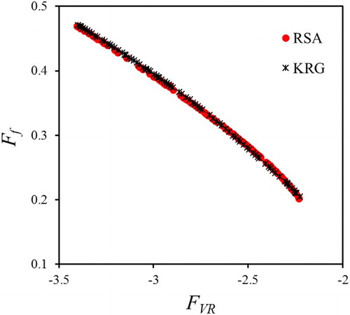
Figure 7. Representative Pareto-optimal designs.

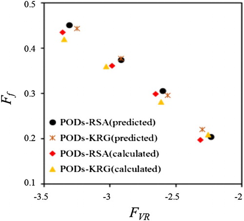
Table 3. Design variables and objective function values at four cluster points and the reference design.

	Design variables		Surrogate prediction		URANS calculation		Relative error [%]
Cluster	w/dth	ds/dth	FVR	Ff	FVR	Ff	FVR	Ff
RSA-A	0.932	0.628	−3.309	0.452	−3.362	0.435	1.58	3.85
RSA-B	0.931	0.904	−2.916	0.374	−2.986	0.362	2.33	3.49
RSA-C	0.933	1.192	−2.602	0.306	−2.653	0.299	1.92	2.39
RSA-D	0.933	1.608	−2.234	0.204	−2.315	0.198	3.4	3.34
KRG-A	0.932	0.663	−3.252	0.444	−3.349	0.420	2.89	5.83
KRG-B	0.932	0.901	−2.917	0.378	−3.029	0.360	3.68	5.03
KRG-C	0.932	1.233	−2.564	0.296	−2.612	0.281	1.84	5.24
KRG-D	0.932	1.679	−2.301	0.221	−2.255	0.209	2.05	5.32
Reference	0.370	1.450	–	–	−1.226	0.221	–	–

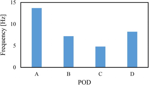
Figure 8 shows the frequency of flow oscillation from the feedback channels for the PODs–RSA (PODs hereafter). The feedback channel was an optimal location to measure the main frequency of the flow oscillation because of the simple flow pattern (Yang et al., 2007). The frequency reached a minimum value at POD C with variations in d_s/d_th. This result implied that the time scale of the oscillation process depended on the distance between the splitters. A higher frequency indicated a smaller residence period of circulating flow in the chamber and a shorter oscillation period (Yang et al., 2007). In the airfoil application for separation control, the most effective oscillation frequency of the fluidic oscillator depended on various conditions including freestream conditions (Scott Collis, Joslin, Seifert, & Theofilis, 2004) and amplitude of oscillating jet (Hecklau et al., 2011; Nishri & Wygnanski, 2004).

Figure 8. Frequency of flow oscillation at the feedback channels.

Time-resolved mass flow rate and time-averaged mass flow rate through right-hand side feedback channels for the PODs are shown in Figure 9 and Table 4, respectively. As shown in Figure 9, PODs A and D have relatively high frequencies of flow oscillation compared with PODs B and C. The lowest frequency design (POD C) exhibited the highest time-averaged mass flow rate through the feedback channels. However, the highest frequency design (POD A) exhibited the lowest time-averaged mass flow rate through the feedback channel. The percentages of the time-averaged mass flow rate through the right-hand side feedback channel with respect to the total mass flow rate through the inlet nozzle for PODs A and C were 21.58% and 22.46%, respectively.

Figure 9. Time-resolved mass flow rate through a right-hand side feedback channel for the PODs.

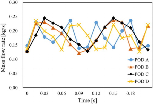
Table 4. Time-averaged mass flow rate through the right-hand side feedback channel for the PODs.

	POD A	POD B	POD C	POD D
Time-averaged Mass flow rate [kg/s]	0.179	0.183	0.187	1.181

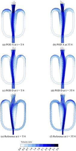
Figure 10 shows the local velocity ratio distributions and velocity vectors at t = T/4 and 3T/4 on the central x-y plane (z = 0) for POD A, POD D, and the reference design. The local velocity ratio was defined as a ratio of local velocity to the reference velocity (U_ref). As shown in Figures 10(a) and (b), the velocity ratio-oriented design (that is, POD A) did not have a throat in the outlet nozzle (d_s/d_th < 1.0) and exhibited the largest region of high local velocity ratio downstream of the splitters. This contributed to the largest peak jet velocity at the outlet in POD A. Conversely, POD D exhibited lower local velocity ratios in the outlet nozzle compared with those in POD A. The reference design displayed the lowest velocity ratios in the same region. The reference design shows the largest region of low velocity in the chamber, and thus the deflection of the main stream also becomes the largest. On the contrary, due to the smallest region of low velocity in the chamber, the deflection of the main stream is minimized in POD A resulting in the largest peak jet velocity at the outlet.

Figure 10. Local velocity ratio distributions and velocity vectors at t = T/4 and 3T/4 on the central x-y plane (z = 0) for POD A, POD D, and the reference design.

The distributions of vorticity in the z-direction (ω_z) at t = T/4 on the central x-y plane (z = 0) for POD A, POD D, and the reference design, are shown in Figure 11. As widely known, a high overall vorticity leads to a large pressure drop (Liu, Wang, & Liu, 2006). In this respect, POD A which shows the largest pressure drop (i.e. the largest F_f) exhibited the largest overall level of absolute vorticity and also the largest variation of vorticity across the outlet nozzle downstream of the splitters.

Figure 11. Vorticity (ω_z) distributions at t = T/4 on the central x-y plane (z = 0) for POD A, POD D, and the reference design.

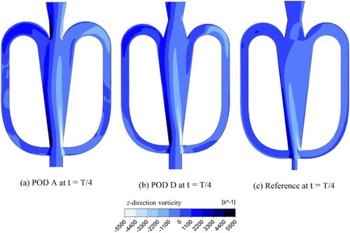
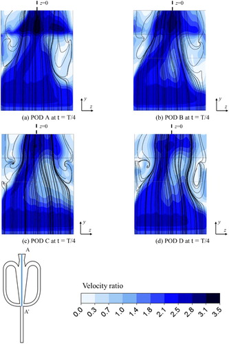
Figure 12 shows the local velocity ratio distributions and streamlines at time t = T/4 on a cross-sectional plane (plane A-A’) for the selected PODs. The working fluid flows upward (positive y-axis direction). It is observed that the local velocity distributions were qualitatively similar for the selected PODs. The geometry of the fluidic oscillator was symmetric about the central x-y plane. Nevertheless, the flow structures were asymmetric and the highest local velocities were observed around z = 0 at the outlet. Among the PODs, POD A included the largest region of high local velocity ratio between the splitters and the outlet, and this was consistent with the distribution on x-y plane as shown in Figure 10(a).

Figure 12. Local velocity ratio distributions and streamlines at t = T/4 on the cross-sectional plane A-A’.

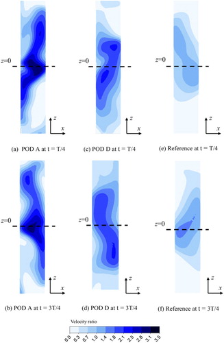
The local velocity distributions at t = T/4 and 3T/4 on the outlet plane for POD A, POD D, and the reference design, are represented in Figure 13. The maximum local velocities were commonly observed around the center of the plane (x = 0 and z = 0) irrespective of the time. This indicated that there were no serious oscillations along the two central lines at x = 0 and z = 0. However, the distributions were asymmetric about these two central lines, and thus oscillation occurred at the other x and z lines. Additionally, the amplitude of oscillation increased as a line moved away from the center. As shown in Figures 13(a) and 13(b), the velocity ratio-oriented design (that is, POD A) exhibited the highest peak velocity and the highest local velocity variation among the tested three cases. This was consistent with the distributions shown in Figures 10 and 12.

Figure 13. Local velocity ratio distributions at t = T/4 and 3T/4 on outlet plane for POD A, POD D, and the reference design.

6. Conclusion

In this study, the multi-objective optimization of a fluidic oscillator was performed using surrogate modeling and an MOGA algorithm with 3D unsteady RANS analysis. The results of analysis with three different turbulence models (k-ε, SST, and BSL) for the frequencies measured from the feedback channel were compared to those in the experimental data. The results indicated that the k-ε model showed the best overall agreement with the experimental data, and it was used for further calculations in the study. With respect to the optimization, two design variables, namely the ratio of the inlet nozzle width (w/d_th) and the distance between splitters (d_s/d_th) to throat width, were selected among the various geometric parameters affecting the performance of the fluidic oscillator. The optimization aimed to simultaneously minimize the following two objective functions: the negative of the peak jet velocity ratio at the outlet (F_VR) and the friction factor through the fluidic oscillator (F_f). The values of the two objective functions were numerically evaluated by using a 3D unsteady RANS analysis at 10 design points selected by LHS to construct surrogate models for the objective functions. To ensure better prediction accuracy of the surrogate models, both the RSA and KRG models were tested. The findings revealed that the RSA model exhibited better prediction accuracies for the optimum objective functions with maximum relative errors of 3.85% compared to the unsteady RANS calculation using the KRG model. Analysis of the four representative PODs showed that the objective functions were sensitive to the design variable d_s/d_th. With respect to moving along the POF in the direction to a higher velocity ratio (forward POD A), the PODs indicated smaller d_s/d_th values with nearly invariant w/d_th values. The jet velocity-oriented design (that is, POD A) did not have a throat in the outlet nozzle (d_s/d_th < 1.0) and represented the largest region of high local velocity ratio from the splitters to the outlet surface. Meanwhile, the largest variation of vorticity occurred at the same region. These flow structures were related to the highest F_VR and the lowest F_f. Consequently, a small d_s/d_th enhanced F_VR, whereas a large d_s/d_th reduced F_f. The jet velocity-oriented design increased F_VR and F_f by 11.18% and 16.82%, respectively, compared to those of the friction factor-oriented design (that is, POD D). The results of the present investigation would provide useful information for the design of a fluidic oscillator required to control a specific external flow. In future works, interaction between the jet issuing from a fluidic oscillator and external flow over an airfoil, is required to be analyzed and optimized to improve the control of the external flow.

Nomenclature

b	=	Feedback channel width (mm)
BSL	=	Baseline turbulence model
Dh	=	Hydraulic diameter of the throat (mm)
DOE	=	Design-of-experiment
ds	=	Distance between splitters (mm)
dth	=	Throat width (mm)
Ff	=	Objective function related to the pressure drop
FVR	=	Objective function related to peak jet velocity at the outlet
H	=	Fluidic oscillator depth (mm)
KRG	=	Kriging
LHS	=	Latin hypercube sampling
	=	Mass flow rate (kg/s)
MOGA	=	Multi-objective genetic algorithm
POD	=	Pareto-optimal design
POF	=	Pareto-optimal front
	=	adjusted coefficient of multiple determination in the polynomial regression
RMS	=	Root-mean square
RSA	=	Response surface approximation
S	=	Distance from the inlet to outlet plane (mm)
SST	=	Shear stress transport
t	=	Time
T	=	Oscillation period
Upeak	=	Maximum jet velocity during the oscillation period (m/s)
URANS	=	Unsteady Reynolds averaged Navier-Stokes
Uref	=	Reference velocity (m/s)
w	=	Inlet nozzle width (mm)
Δp	=	pressure drop (Pa)

Greek letters
ρ	=	Density (kg/m­3)
ωz	=	z-direction vorticity (s−1)

Disclosure statement

No potential conflict of interest was reported by the authors.

References

- ANSYS. (2013). CFX-15, solver theory. Canonsburg, PA: ANSYS Inc.
- Burns, A. (2015). Turbine tip clearance control using fluidic oscillators (Doctoral dissertion). Retrieved from http://kuscholarworks.ku.edu/handle/1808/19426
- Cerretelli, C., Wuerz, W., & Gharaibah, E. (2010). Unsteady separation control on wind turbine blades using fluidic oscillators. AIAA Journal, 48(7), 1302–1311. doi: 10.2514/1.42836
- Deb, K., Pratap, A., Agarwal, S., & Metarivan, T. (2002). A fast Elist multiobjective genetic algorithm: NSGA-II. Computer Methods in Applied Mechanics and Engineering, 196(4), 879–893.
- Ezhilsabareesh, K., Rhee, S. H., & Samad, A. (2017). Shape optimization of a bidirectional impulse turbine via surrogate models. Engineering Applications of Computational Fluid Mechanics. Advanced online publication. doi: 10.1080/19942060.2017.1330709
- Gao, T., Wang, Y., Pang, Y., & Cao, J. (2016). Hull shape optimization for autonomous underwater vehicles using CFD. Engineering Applications of Computational Fluid Mechanics, 10(1), 599–607. doi: 10.1080/19942060.2016.1224735
- Goel, T., Vaidyanathan, R., Haftka, R. T., Shynn, W., Queipo, N. V., & Tucker, K. (2007). Response surface approximation of Pareto optimal front in multi-objective optimization. Computer Methods in Applied Mechanics and Engineering, 196(4), 879–893. doi: 10.1016/j.cma.2006.07.010
- Greenblatt, D., & Wygnanski, I. J. (2000). The control of flow separation by periodic excitation. Progress in Aerospace Sciences, 36(7), 487–545. doi: 10.1016/S0376-0421(00)00008-7
- Hecklau, M., Wiederhold, O., Zander, V., King, R., Nitsche, W., Huppertz, A., & Swoboda, M. (2011). Active separation control with pulsed jets in a critically loaded compressor cascade. AIAA Journal, 49(8), 1729–1739. doi: 10.2514/1.J050931
- Husain, A., Lee, K.-D., & Kim, K.-Y. (2011). Enhanced multi-objective optimization of a dimpled channel through evolutionary algorithms and multiple surrogate methods. International Journal for Numerical Methods in Fluids, 66(6), 742–759. doi: 10.1002/fld.2282
- Jeong, H.-S., & Kim, K.-Y. (2016). Effects of fluidic oscillator geometry on performance. Journal of Computational Fluids Engineering, 21(3), 77–88. doi: 10.6112/kscfe.2016.21.3.077
- Joen, M. K., Kim, J.-H., Noh, J., Kim, S.-H., Park, H. G., & Woo, S. I. (2005). Design and characterization of a passive recycle micromixer. Journal of Micromechanics and Microengineering, 15, 346–350. doi: 10.1088/0960-1317/15/2/014
- Kim, H.-M., & Kim, K.-Y. (2006). Shape optimization of three-dimensional channel roughened by angled ribs with RANS analysis of turbulent heat transfer. International Journal of Heat and Mass Transfer, 49(21–22), 4013–4022. doi: 10.1016/j.ijheatmasstransfer.2006.03.039
- Kim, J., Moin, P., & Seifert, A. (2015). LES-based characterization of a suction and oscillatory blowing fluidic oscillator. Bulletin of the American Physical Society, 60, 157–168.
- Kim, K.-Y., & Lee, Y.-M. (2007). Design optimization of internal cooling passage with V-shaped ribs. Numerical Heat Transfer, Part A: Applications, 51(11), 1103–1118. doi: 10.1080/10407780601112860
- Lee, K. Y., Chung, H. S., Cho, D. H., & Shon, M. H. (2007). Flow separation control effects of blowing jet on an airfoil. Journal of the Korean Society for Aeronautical and Space Sciences, 35(12), 1059–1066. doi: 10.5139/JKSAS.2007.35.12.1059
- Lee, S. M., & Kim, K. Y. (2015). Multi-objective optimization of arc-shaped ribs in the channels of a printed circuit heat exchanger. International Journal of Thermal Sciences, 94, 1–8. doi: 10.1016/j.ijthermalsci.2015.02.006
- Liu, C., Wang, L., & Liu, Q. (2006). A universal approach for mean mechanical energy losses analysis. Chemical Engineering Science, 61(6), 2085–2088. doi: 10.1016/j.ces.2005.10.011
- Martin, J. D., & Simpson, T. W. (2005). Use of Kriging models to approximate deterministic computer models. AIAA Journal, 43(4), 853–863. doi: 10.2514/1.8650
- McKay, M. D., Beckman, R. J., & Conover, W. J. (2000). A comparison of three methods for selecting values of input variables in the analysis of output from a computer code. Technometrics, 42(1), 55–61. doi: 10.1080/00401706.2000.10485979
- Menter, F. R. (1993). Zonal two equation k-w turbulence models for aerodynamic flows (AIAA paper, 2906).
- Myers, R. H., Montgomery, D. C., & Anderson-Cook, C. M. (2016). Response surface methodology process and product optimization using designed experiments. New York: John Wiley and Sons.
- Nagib, H., Kiedaisch, J., Reinhard, P., & Demanett, B. (2006). Control techniques for flows with large separated regions: A new look at scaling parameters (AIAA paper, 2006(2857)).
- Nishri, B., & Wygnanski, I. (2004). Active management of naturally separated flow over a solid surface. Part 1. The forced reattachment process. Journal of Fluid Mechanics, 510(7), 105–129.
- Ostermann, F., Woszidlo, R., Nayeri, C., & Paschereit, C. O. (2015, January). Experimental comparison between the flow field of Two common fluidic oscillator design. 53rd AIAA aerospace science meeting, Kissimmee, Florida.
- Panitz, T., & Wasan, D. T. (1972). Flow attachment to solid surfaces: The Coanda effect. AIChE Journal, 18(1), 51–57. doi: 10.1002/aic.690180111
- Papila, N., Shyy, W., Griffin, L. W., & Dorney, D. J. (2011). Shape optimization of supersonic turbines using response surface and neural network methods (AIAA paper, 2001(1065)).
- Queipo, N. V., Haftka, R. T., Shyy, W., Goel, T., Vaidyanathan, R., & Tucker, P. K. (2005). Surrogate-based analysis and optimization. Progress in Aerospace Sciences, 41(1), 1–28. doi: 10.1016/j.paerosci.2005.02.001
- Sack, J., Welch, W. J., Mitchell, T. J., & Wynn, H. P. (1989). Design and analysis of computer experiments. Statistical Science, 4(4), 409–423. doi: 10.1214/ss/1177012413
- Scott Collis, S., Joslin, R. D., Seifert, A., & Theofilis, V. (2004). Issues in active flow control: Theory, control, simulation, and experiment. Progress in Aerospace Sciences, 40(4), 237– 289. doi: 10.1016/j.paerosci.2004.06.001
- Seele, R., Graff, E., Lin, J., & Wygnanski, I. (2013). Performance Enhancement of a Vertical Tail Model with Sweeping Jet Actuators (AIAA paper, 2013(411)).
- Taormina, R., & Chau, K. (2015). Data-driven input variable selection for rainfall-runoff modeling using binary-coded particle swarm optimization and extreme learnig machines. Journal of Hydrology, 529(3), 1617–1632. doi: 10.1016/j.jhydrol.2015.08.022
- Tesar, V. (2015). High-frequency fluidic oscillator. Sensors and Actuators A: Physical, 234, 158–167. doi: 10.1016/j.sna.2015.08.019
- Vasta, V., Koklu, M., Wygnanski, I., & Fares, E. (2012). Numerical simulation of fluidic actuators for flow control applications (AIAA Paper, 2012(3239)).
- Wang, W.-c., Chau, K.-w., Xu, D.-m., & Chen, X.-Y. (2015). Improving forecasting accuracy of annual runoff time series using ARIMA based on EEMD decomposition. Water Resources Management, 29(8), 2655–2675. doi: 10.1007/s11269-015-0962-6
- Warren, R. W. (1960). US Patent No. 3,016,066 Washington, DC: U.S. Patent and Trademark Office.
- Woszidlo, R., & Wygnanski, I. (2011). Parameters governing separation control with sweeping jet actuators (Doctoral Dissertion). Retrieved from: http://arizona.openrepository.com/arizona/handle/10150/203475
- Xu, C., & Meng, X. (2013). Performance characteristic curve insensitive to feedback fluidic oscillator configurations. Sensors and Actuators A: Physical, 189, 55–60. doi: 10.1016/j.sna.2012.09.031
- Yang, J.-T., Chen, C.-K., Tsai, K.-J., Lin, W.-Z., & Sheen, H.-J. (2007). A novel fluidic oscillator incorporating step-shaped attachment walls. Sensors and Actuators A: Physical, 135(2), 476–483. doi: 10.1016/j.sna.2006.09.016
- You, D., & Moin, P. (2008). Active control of flow separation over an airfoil using synthetic jets. Journal of Fluids and Structures, 24(8), 1349–1357. doi: 10.1016/j.jfluidstructs.2008.06.017
- Zhang, J., & Chau, K. (2009). Multilayer ensemble pruning via novel multi-sub-swarm particle swarm optimization. Journal of Universal Computer Science, 15(4), 840–858.