Numerical simulation of scour around circular piles due to unsteady currents and oscillatory flows

ABSTRACT

Numerical modeling of pile scour is performed due to the action of unsteady currents and oscillatory flow greens, using 3D Reynolds averaged Navier–Stokes (RANS) equations for the hydrodynamic description and the Exner equation for the morphological evolution of the bed, all of them incorporated into the computational fluid dynamics tool called REEF3D. As a first task, the numerical model was calibrated by comparing its results of scour against two sets of data, the first one obtained from numerical simulations and the second one from experimental tests. From these results it was possible to define the closure model of turbulence and a relaxation coefficient on the bed load equation necessary to increase the mobility of the sediments in the vicinity of the pile. Once the model was calibrated, a set of numerical simulations of pile scour under unsteady flow and oscillatory flow was performed using different hydrographs and wave conditions. There is a strong agreement between the simulated data and the experimental data reported by other authors for unsteady flow. In the case of scour associated with oscillatory flow, the numerical results showed the same statistical behavior as the experimental data previously published by others. When the numerical results are analyzed according to the Keulegan-Carpenter number, they represent the scour phenomenon in the same order of magnitude of the experiments. A conclusion of the study is the necessity to improve the sediment transport description, in order to avoid the use of a dedicated relaxation coefficient that reduces the threshold condition of the incipient transport.

KEYWORDS:

• Computational fluid dynamics
• cylindrical pile
• scour
• unsteady flow
• oscillatory flow
• REEF3D

1. Introduction

The scour process around a cylindrical pile founded on a riverbed composed of non-cohesive granular material corresponds to a mechanism in which the hydrodynamics behavior of the fluid and sediment transport are highly influenced by the presence of the obstacle, changing the bottom bed shear stresses near the pile and causing the scour of the bed.

In pile scour studies, two different terms are commonly used: clear-water condition and live bed condition. The first of them refers to the condition in which the flow velocity near the bed is less than the incipient threshold and the sediment transport are just developed in the vicinity of the pile. The live-bed regime is the condition in which the flow velocity (shear stress) near the bed is greater than the incipient threshold.

A grain of sediment needs a higher bed shear stress to suspend than to move as a bed load (Van Rijn, 1984b), thus, in a pile scour study, a clear water condition is not able to produce suspended load, due to the fact that in this kind of regimen the bed shear stress is less than the critical value associated with the sediment.

The pile obstructs the flow and modifies the hydrodynamic behavior in comparison with the free stream case, forming the so-called horseshoe vortex and vortex shedding in the neighborhood of the pile, which have been historically described by Baker (1979) for the laminar case, and Baker (1980) and Sumer and Fredsøe (2002) for the turbulent one. In oscillatory flows something analogous happens, which is described by Sumer, Fredsøe, and Christiansen (1992) and Sumer, Christiansen, and Fredsøe (1997).

The vortex system that develops around cylindrical piles is the hydrodynamic mechanism that produces the scour near a pile. This has been observed previously by many authors, for example Breusers, Nicollet, and Shen (1977) describes in their state-of-art research that since Keutner (1932) the scour has been associated to the horseshoe vortex, which is concordant with the work carried out by Tison (1940), Posey (1949), Laursen & Toch (1956), Roper, Schneider, and Shen (1967) and Melville (1975), among others.

The horseshoe vortex and its relationship with the scour hole are still under study, both experimentally (S. Das, Das, & Mazumdar, 2013; Dey & Raikar, 2007; Unger & Hager, 2007) and numerically (Baykal, Sumer, Fuhrman, Jacobsen, & Fredsøe, 2015; Link, Gobert, Manhart, & Zanke, 2008a; Roulund, Sumer, Fredsøe, & Michelsen, 2005).

The numerical modeling of cylindrical pile scour due to steady and oscillatory flows has been previously studied by several authors, focusing their efforts both in the correct description of the horseshoe vortex and vortex shedding, and in the quantification of the bed level change around the structure, because experimentally it has been demonstrated that these two vortices are responsible for pile scour. Sumer and Fredsøe (2002), based on the compilation of previous works on numerical modeling of fluid–pile interactions, indicate that one of the most important aspects in the representation of the scouring is the hydrodynamic description of the horseshoe vortex and vortex shedding, which generally come from the solution of Reynolds averaged Navier–Stokes (RANS) equations with a turbulence model for closure or another more complex approximation, e.g. direct numerical simulations (DNS), large-eddy simulations (LES) or detached-eddy simulation (DES).

For steady flows, Olsen and Melaaen (1993) developed a three-dimensional numerical model to solve the hydrodynamic and the bed level change around the cylindrical pile, incorporating as turbulence closure the model, while the sediment transport was determined by an advection-diffusion approximation of the sediment continuity equation. The numerical results of Olsen and Melaaen (1993) were compared with data obtained in laboratory experiments, showing agreement between both of them (Sumer & Fredsøe, 2002).

Complementary to the Olsen and Melaaen (1993) work, Roulund et al. (2005) proposed a three-dimensional numerical model to solve RANS equations for a pile scour with a turbulence closure model given by the equations, and compared their hydrodynamic and scour results against experimental data obtained in the laboratory. The results show that the numerical simulation developed captures all the main features of the scour process, including the equilibrium scour depth, that agree well with the experiments for the upstream scour hole, but some discrepancy was observed at the downstream (30% of differences between the modeled scour and the measurements, according to estimations of Roulund et al. (2005)).

The Lagrangian approach to estimate the scour around cylindrical piles due to steady flow is applied by Liu and García (2008) and Escauriaza and Sotiropoulos (2011). The former orientates this technique on the definition of a grid which adapts to the variations of the river-bed, whilst the latter is focused on the determination of movement particle by particle.

The Lagrangian techniques have also been applied to the simulation of non-Newtonian flows, in order to estimate their rheology. One of the recent applications of this technique was the one presented by Xie and Yee-Chung (2016).

In the case of oscillatory flows, Kobayashi (1992) developed a three-dimensional numerical model to explain the flow around cylindrical piles. However, the model solely reviewed the generation of vortex sheddings, but no horseshoe vortex, without further explaining how to determine the bed level change. Later, the aspects excluded by Kobayashi (1992) were incorporated by Yuhi, Ishida, and Umeda (2000).

Related to sediment transport and its modeling, Roulund et al. (2005) acknowledge the existence of three fundamental aspects to incorporate to the numerical models of pile scour: sediment transport as a bed load, sand slide and the conservation of sediment. With respect to bed load, Roulund et al. (2005) in Sumer (2007) comments that it is usual to employ bidimensional conventional equations, which are also used for sediment avalanches. The conservation of sediment is usually approached by the vectorization of Exner's equation (x and y directions), which shows bed variations over time. In the mean time, for the turbulence closure, the use of the model is recommended based on the results presented by Menter (1994). However Olsen & Kjellesvig (1998) obtained good agreement with empirical equations by employing the closure model into the RANS equations to estimate the maximum scour depth.

An additional sediment transport mechanism that can be present in the pile scour is backfilling. This corresponds to the sedimentation in the downstream region of the pile. However, very few studies regarding this phenomenon have been published, e.g. Sumer et al. (2013) (experimental) and Baykal, Sumer, Fuhrman, Jacobsen, & Fredsøe (2017) (numerical). In both cases the live bed regimen is considered.

Recently, a numerical study of flow around circular piers using the closure model in the RANS equations was carried out by Baranya, Olsen, Stoesser, and Sturm (2012). In this study, three pier arrangements were simulated: flow around a single pier, and flows around two piers placed in two different layouts. The hydrodynamical results were validated using measurements obtained from an acoustic Doppler velocimeter (ADV). Baranya et al. (2012) highlight results which indicate that for a single pier simulation the vertical velocity profiles have a good agreement with the ADV data. However, a slight underestimation of the velocities is expected in the downstream region.

Several open access numerical tools for computational fluid dynamics (CFD) are available, e.g. OpenFoam® (https://www.openfoam.com/), SPHysics (http://dual.sphysics.org/index.php/sphysics-project/), Fluidity (http://fluidityproject.github.io/) and REEF3D (https://reef3d.wordpress.com/). These models have been applied to many different cases. For example, OpenFoam has been applied to simulate pile scour (Liu & García, 2008), flow structure interaction (Doolan, 2010; Haque, Katsuchi, Yamada, & Nishio, 2016) and particle tracking, for studying particle-laden flows (Greifzu, Kratzsch, Forgber, Lindner, & Schwarze, 2016).

SPHysics is a model based on smoothed particle hydrodynamics (SPH) developed jointly by researchers at the Johns Hopkins University, the University of Vigo, the University of Manchester and the University of Rome La Sapienza. This model has been applied to simulate water waves (Altomare et al., 2015; Dalrymple & Rogers, 2006), sedimentation, resuspension and scour (Fourtakas & Rogers, 2016; Saghatchi, Ghazanfarian, & Gorji-Bandpy, 2014), among other applications.

Fluidity is a CFD model developed by Imperial College, which has been applied to simulate multiphase flows (Jacobs et al., 2015), tsunami propagation (Oishi et al., 2013) and geodynamics Davies, Wilson, and Kramer (2011), among others.

The REEF3D numerical model resulted from doctoral research work by Bihs (2011). In its first version it was capable of determining the hydrodynamic, sediment transport and bed changes, under steady flow. Bihs (2011) applied the model to simulate the scour around cylindrical piles under steady flow. Later versions of the numerical model include the capability to simulate oscillatory flow (Saud, 2013).

An application of the REEF3D model to simulate the pile scour under oscillatory flow was performed by Ahmad, Bihs, Kamath, & Arntsen (2015), who considered monopile and pile group in their simulation. Another application to sediment transport was developed by Afzal, Bihs, Kamath, and Arntsen (2015) who applied the model to simulate pile scour under current and waves.

There are several numerical models, which have been applied to simulate various phenomena, such as hydrodynamics (Brevis, García-Villalba, & Niño, 2014; Ulloa, Winters, de la Fuente, & Niño, 2015), water quality (Chau & Jiang, 2001, 2004; Wu & Chau, 2006), and non-Newtonian flow (Greifzu et al., 2016; Özkan, Wenka, Hansjosten, Pfeifer, and Kraushaar-Czarnetzki, 2016; Trewhela, Ihle, & Tamburrino, 2014; Xie & Yee-Chung, 2016). However, it is not the aim of this article to describe each application of the numerical models and we just are focused on the applications to the pile scour simulation.

A review of the last 20 years of literature of pile scour shows that the clear water condition (such that the scour reaches it is maximum value according to Melville (2008)) has been used for the numerical estimations of the scour around piles. That is to say, the flow condition corresponds to the threshold for sediment transport.

The time scales involved in the scouring process to reach equilibrium due to steady flow may vary from days to weeks (Melville & Chiew, 1999; Oliveto and Hager, 2002); whilst for the oscillatory flows the time for equilibrium should be about 1000 times the wave period (Kobayashi & Oda, 1994). In both cases (steady flow and oscillatory flow) the requirement for reaching the scour equilibrium is that the flow remains constant during the whole period (time scale). However, as is well known, the river discharge or waves in a beach, associated with a flood or extreme climate, have a limited duration, and so some authors have begun to develop experiments to measure the temporal distribution influence in the scour around piles.

In order to analyze the time dependence of the bed change around of a pile due to unsteady flows, most studies have approached the study experimentally, by testing the effect of hydrographs on the local scour (Chang, Lai, & Yen, 2004; Gjunsburgs, Jaudzems, & Govša, 2010; Kothyari, Garde, & Ranga Raju, 1992; Link et al., 2017; Melville & Chiew, 1999; Mia & Nago, 2003; Oliveto and Hager, 2002). In the case of oscillatory flows, studies on the determination of scour are scarce and the inclusion of the temporal scale is reduced to a couple of experimental works (Kobayashi & Oda, 1994; Sumer & Fredsøe, 2002).

The main objective of this paper is to model numerically the scour around cylindrical piles due to unsteady current and oscillatory flow, by applying Eulerian techniques when defining sediment transport and regular grids for the numerical solution of the hydrodynamics around the structure.

In order to achieve that objective, a series of specific activities were followed, oriented to obtaining numerical results. As a first task, REEF3D was compared against numerical and experimental results obtained by other authors, in order to verify the numerical tool capability to represent the scour around circular piles under steady flow. The second task was developed to verify the numerical tool capability to represent the scour around circular piles under unsteady flow, against experimental results obtained by other authors. The last task was to compare the numerical results from the scour due to oscillatory flow against experimental data in the available literature.

This study aims to provide a numerical background for studies of scour around circular piles, for temporal scales smaller than those necessary to reach the equilibrium scour.

2. Materials and methods

2.1. REEF3D numerical model

REEF3D v15.12 (Bihs, 2011; Saud, 2013) was employed in order to run the numerical simulation. It is a CFD model and has been developed with the capability to study hydraulic, coastal and estuarine phenomena, for both compressible and incompressible fluids.

The model solves the RANS three-dimensional equations (Reynolds, 1895) by applying the finite differences method on a squared-element grid, with turbulence closure models: (Launder & Sharma, 1974) and (Wilcox, 1998).

The RANS three-dimensional equations solved by REEF3D are then shown. Equation (1(1) ) corresponds to the continuity for an incompressible flow and Equation (2(2) ) to the momentum conservation: (1) (2) where i, j=1,2,3, is the mean velocity vectorial component, is the spatial vectorial component, t is the time, ρ is the water density, p is the pressure, ν is the kinematic viscosity, is the kinematic eddy viscosity and g is the gravity.

The closure models for used ( and ) are described in the next equations. The closure model defines the turbulent viscosity () according to Equation (3(3) ) in which is a constant value equal to 0.09 (Launder & Spalding, 1974), k is the turbulent kinetic energy, and ε is the turbulent dissipation. (3)

Both the turbulent kinetic energy and the turbulent dissipation are determined with a transport equation according to Equations (4(4) ) and (5(5) ), where , , and are constant values equal to: 1, 1.3, 1.44 and 1.92, respectively, according to Launder and Spalding (1974). is the turbulent production rate given by Equation (6(6) ). (4) (5) (6)

In the case of the closure model, the turbulent viscosity () is defined according to Equation (3(3) ), and both the turbulent kinetic energy (k) and the specific turbulent dissipation (ω) are determined with a transport equation, according to Equations (8(8) ) and (9(9) ), where , , , and is the turbulent production rate given by Equation (6(6) ). (7) (8) (9)

Due to the model use of the Cartesian grid, a special treatment is used to solve the flow around complex structures and geometries. This is called the ghost cell method (Berthelsen, 2004; Tseng & Ferziger, 2003). This corresponds to a method for imposing the boundary conditions necessary for the numerical simulation of obstacles submerged in the fluid. This approach uses fictional cells, that are incorporated in the domain (specifically on the obstacles) and corresponds to a particular case of the immersed boundary method (Leveque and Li, 1994).

Since this method extrapolates the solution into the immersed obstacle, the boundary conditions are implicitly incorporated into the numerical discretization, and so do not need to be accounted for explicitly in the grid cell definition.

The temporal discretization of the governing equations was solved by applying the Runge–Kutta method (second order). For the convective terms, the WENO (weighted essentially non-oscillatory) scheme was implemented (Jiang and Shu, 1996). The velocities and pressures are determined under a staggered grid, and the SIMPLE (Patankar and Spalding, 1972) or PISO method (Issa, 1986) is applied when incorporating the pressure gradients in the problem governing equations. For this application the SIMPLE method was used as pressure algorithm.

Additional information regarding the boundary condition and initialization used as a general definition for REEF3D configuration is shown in Table 1.

Table 1. Complementary information for the REEF3D general configuration for the hydrodynamics simulation.

Configuration	Definition
Boundary condition	Non-slip for velocities
	Non-slip for k, ω and ε
	Logarithmic profile for inlet flow
	Fix pressure at inlet
	Zero-gradient outflow
Initialization	Potential flow for velocities
	Hydrostatic for pressure

REEF3D has the capability to calculate sediment transport as bed load, suspended load and sandslide. For the bed load it is possible to employ the equations of Meyer-Peter and Müller (1948), Engelund and Fredsøe (1976) or Van Rijn (1984a). The suspended solids are estimated from the advection-diffusion equation of the sediment concentration. The sandslide correspond to a mechanism of sediment transport regarding to the slope instability of the bed and is determined according to Burkow (2010).

In this study only the bed load is considered, due to the grain size of the sediment, and was determined using the Meyer-Peter and Müller (1948) equation: (10) where is the dimensionless bed load, is the dimensionless shear stress on the bed, is the dimensionless critical shear stress and the dimensionless magnitudes are: (11) (12) (13) where τ and are the shear stress and the critical shear stress, is the bed load, is the sediment density, ρ is the fluid density, d is the sediment diameter and g is gravity acceleration.

The critical shear stress is computed from the Shields (1936) diagram for a flat bed parameterized by Yalin (1972), incorporating the slope corrections proposed by Dey (2001). Moreover, as an additional sediment transport mechanism, the sandslide effect was considered according to the Burkow (2010) (in  Saud, 2013).

The reduction of the incipient shear stress due to the bed slope proposed by Dey (2001) is based on taking the Shields critical shear stress for a flat horizontal bed () and using a coefficient (r), according to the following expressions: (14) (15) where θ and α are the longitudinal and transversal angles of slope, respectively, and φ is the angle of repose. It is important to note that this incipient shear stress reduction must be applied when the bed has a slope, otherwise r=1.

Additionally, a relaxation coefficient () is incorporated over the bed, which allows regulation of the particle behavior due to hydrodynamics action. Thus it increases the sediment mobility in particular zones within the numerical domain, as was presented by Bihs (2011).

The relaxation coefficient is implemented numerically in REEF3D, affecting the dimensionless critical shear stress () according to the following expression: (16) where corresponds to the area in which the relaxation coefficient < 1 wants to be applied.

To define the area in which the relaxation coefficient must to be applied, a preliminary estimation of the equilibrium scour hole was made according to Link, Pfleger, and Zanke (2008b) and Diab, Link, and Zanke (2010).

To determine the bed level change due to the hydrodynamics and the sediment transport, the conservation of sediment equation is applied. It was initially proposed by Exner (1925) and later generalized by Paola and Voller (2005) in accordance to the following equation: (17) where n is the porosity of the bed, is the bed elevation, and and are the sediment transport as bed load in the x and y directions, respectively, which are determined according to: (18) (19) (20) (21) (22) where and are the x and y components of the total shear stress (), is a constant coefficient related to friction (equal to 0.3 according to Saud, 2013) and , and are the flow velocities components in x, y and z directions near the bed (frictional velocities).

Once the bed morphology has been updated according to the bed load action (solution of Exner equation), the sandslide is verified. This is an iterative processes in which the local slope is compared with the repose angle of sediment (φ) according to: (23)

If Equation (23(23) ) is true then the model makes the sediment surface distribution in both directions, longitudinal and lateral, according to the methodology of Burkow (2010). While Equation (23(23) ) is still fulfilled, the sediment surface distribution continued to deform until the local slope (longitudinal and lateral) becomes equal to the repose angle.

The bed level and the free surface locations are treated as fluid–sediment or fluid–atmosphere interfaces, through one of the following methods: level set method (Osher & Sethian, 1988) or particle level set method (Enright, Fedkiw, Ferziger, & Mitchell, 2002), the first of them being the one used in this application.

The level set method is a moving boundary solution both for the free surface and for the bed and due to that, it incorporates or eliminates cells for the flow calculation, according to whether the surface becomes wavy or the bed begins to scour.

To solve the oscillatory flows, REEF3D incorporates the following wave theories: cnoidal wave for 1st and 5th order, solitary wave for 1st and 3rd order, Stokes waves for 2nd and 5th order and linear theory. Any of these wave theories can be used to define the boundary condition at the inlet of the numerical domain.

2.2. Methodology

In this research a total of 17 numerical tests of pile scour were performed. Two of them (CAL01 and CAL02) were calibration tests, five tests (H01 to H05) were simulated under unsteady currents and the last 10 cases (C01 to C10) were defined to represent the pile scour under oscillatory flow.

The general numerical setting of the REEF3D model is summarized in Table 2, including the domain length (L), width (W), depth (h), grid element size (, , ), cell numbers (N Cells), simulated time (t) and computational time (t).

Table 2. Summary of the numerical configuration of REEF3D model, applied to each simulated cases.

Case	L m	W (m)	h (m)	,, (m)	N Cells	t (min)	t(days)
CAL01	0.8	0.6	0.2	0.005	7.68	2	1.1
CAL02	4.0	2.0	0.8	0.025	4.10	1,260	62.3
H01	4.0	1.5	1.0	0.010	6.60	90	5.6
H02	4.0	1.5	1.0	0.010	6.60	47	3.6
H03	4.0	1.5	1.0	0.010	6.60	27	2.1
H04	4.0	1.5	1.0	0.010	6.60	21	2.1
H05	4.0	1.5	1.0	0.010	6.60	360	15.2
C01	15.0	2.0	1.0	0.010	3.00	50	3.4
C02	15.0	2.0	1.0	0.010	3.00	67	4.4
C03	15.0	2.0	1.0	0.010	3.00	50	3.7
C04	15.0	2.0	1.0	0.010	3.00	67	4.6
C05	15.0	2.0	1.0	0.010	3.00	50	3.7
C06	15.0	2.0	1.0	0.010	3.00	67	4.6
C07	15.0	2.0	1.0	0.010	3.00	50	3.8
C08	15.0	2.0	1.0	0.010	3.00	67	4.7
C09	15.0	2.0	2.0	0.010	6.00	84	6.7
C10	15.0	2.0	2.0	0.010	6.00	167	12.4

It is important to mention that the cell numbers indicated in Table 2 are defined as the total cells included in the whole numerical domain. That includes sediment bed, the water column and the air above the water. This way, at each time interval, the computed number of cells can be less than the total cell number. This will vary according to the free surface and bed movements along time.

The simulated time (t) corresponds to the total time to resolve in the model, meanwhile the computational time (t) is the real time employed to solve any case in the used computer (Intel (r) Core (TM) i7-5930k CPU 3.5 GHz, 64.0 GB, 6 cores).

All other details employed to configure each REEF3D simulated case are indicated in sections 2.2.1 and 2.2.2.

2.2.1. Model configuration - calibration test for steady flow

To define a base configuration for the REEF3D model oriented to pile scour simulation, two kinds of calibration tests were performed. The first one was oriented to compare with another numerical simulation (Baykal et al., 2015), meanwhile the second one was oriented to compare with experimental data (Link, 2006). In both cases steady flow was used to simulate the discharge.

2.2.1.1 Numerical behavior

The data obtained from the numerical simulation of pile scour corresponds to Baykal et al. (2015). The reported results corresponds to a numerical study about scour around cylindrical piles founded on a bed of uniform sediment, under the action of a steady flow. The turbulence closure used for was the SST model.

Baykal et al. (2015) provide the temporal evolution information about the maximum scour produced for a uniform flow, made dimensionless by the pile diameter, S/D, for a period of 120 s of simulation, both for the upstream and downstream zones. These time series were compared with the REEF3D generated data.

The numerical simulations in REEF3D were performed considering a rectangular channel 0.8, 0.6 and 0.2 m long, wide and deep, respectively, being those dimensions in agreement with the Baykal et al. (2015) recommendations.

The spacial discretization was determined using the Hirt and Cook (1972) criterion, which relates the cell size ( = = ) with the pile Reynolds number. The time step () was automatically determined by the Courant criterion in the REEF3D model.

Hirt and Cook (1972) present a technique to solve the Navier–Stokes equations by finite differences, considering the temporal variation of the system and the three-dimensional components of the velocity field. Specifically, the authors apply the method called marked and cell method (MAC) in a confined space.

In order to define the optimal cell size to solve the RANS equations, they recommend defining the Reynolds number associated to the pile () and the number of points must be greater than the square root of ().

The water depth in the test channel was 0.08 m, placed over a 0.12 m uniform sediment layer ( = 0.17 mm). The pile diameter was 0.04 m, while the discharge remained constant and equal to 0.02 m s⁻¹ during the whole modeling period as an inlet boundary condition.

To solve the advective terms from the governing equations, the WENO method was employed, while for the pressure incorporation a projection algorithm was used according to the Chorin (1968) methodology. To determine the free surface, the level set method was used, with a temporal discretization by the Runge–Kutta's 3rd order approximation, whilst a Runge–Kutta's 2nd order for the momentum equations was used. This model configuration was used for all the pile scour simulations contained in this research.

The turbulence closure model for the RANS equations was selected between the and , in order to define which of them have the best agreement with the Baykal et al. (2015) data.

The main objective of this calibrating test by comparing numerical data was to verify that the REEF3D model responds similarly to other numerical tools available, as well as to determine the relaxation coefficient () magnitude of the sediment transport and the turbulence closure model to employ.

2.2.1.2 Comparison with experimental data

The data obtained by Link (2006) correspond to experimental results for a clear water condition scour under steady flow, running in a flume 37 m long, 2 m wide and 1 m deep.

In the middle of the flume a pile of 0.2 m of diameter was placed over a bed composed of a uniform sediment ( = 0.97 mm). The water depth tested was 0.3 m and a discharge of 0.18 m³ s⁻¹ acting for 21 h, in order to reach the equilibrium scour.

To represent numerically the experimental data obtained previously by Link (2006), the REEF3D model was set by considering a numerical flume with 4 m length, 2 m wide and 0.8 m depth. The cell size was 0.025 m with a time step automatically defined by the model, according to the Courant criterion.

The turbulence closure model for the RANS equations was selected according to the one that showed the best agreement in the previous calibration test, i.e. in section 2.2.1.1.

The main objective of this test is to calibrate the numerical model, to verify that the results obtained from REEF3D present a good agreement with the experimental data.

A summary of the calibration test is shown in Table 3 in which the scour regimen is also indicated. The live bed condition was obtained for the numerical comparison and the clear water condition was obtained for the experimental comparison.

Table 3. Summary of the calibration test for REEF3D.

Case	Calibration test	Duration (min)		(mm)	(kg m^−3)	φ ()			Regimen
CAL01	Numerical	2.00	0.13	0.18	2650	30	0.06	2.85	Live bed
CAL02	Experimental	1260	0.02	0.97	2650	30	0.03	0.66	Clear water

2.2.2. Pile scour simulation for unsteady current and oscillatory flow

The scour was studied with two kinds of flow conditions. The first of them corresponded to unsteady current defined through hydrographs, while the second corresponded to oscillatory flow generated by regular gravitational waves.

To study the scour around cylindrical piles due the action of unsteady current, five hydrographs previously tested in laboratory by Link et al. (2017) were considered. They provide information about the temporal evolution of the maximum scour for the different length trials. The test performed by Link et al. (2017) took place in the hydraulic laboratory of Universidad de Concepción (Chile), in a rectangular channel of 26, 1.5 and 0.74 m of long, wide and deep, respectively. The employed pile had 0.15 m of diameter made out of Plexiglas. An electronic distance measurement (EDM) laser allowed measurement of the scour around the pile with a precision of ± 0.4 mm. The bed was composed of a = 0.36 mm diameter sand with a geometrical standard deviation of 1.45 and a density of 2650 kg m.

According to Link et al. (2017), for the sediment used in his experiments the incipient motion occurs at a velocity of 0.32 m s⁻¹. The experiment was conducted under clear water condition, with a maximum discharge of 91% associated to the incipient motion condition. In Link et al. (2017), seven different hydrographs were tested. However, in the present research, just five of them were considered. They were named tests A, B, C, D and E, and are illustrated in Figure 1.

Figure 1. Hydrographs used for the pile scouring simulation under the action of unsteady flow.

Test A corresponds to a staggered hydrograph of 90 min duration, in which the maximum discharge is reached 40 min after the test started and remains constant for another 20 min to decrease for another 20 min. Test B also corresponds to a staggered hydrograph, but with just one growing phase, reaching the maximum discharge 19 min after the test started, remaining constant for another 20 min. The total duration of the experiment was about 49 min. Test C corresponds to a triangular hydrograph lasting around 28 min, with a maximum discharge reached 12 min after the test started. The hydrograph corresponding to test D has a smooth triangular distribution, where the maximum discharge is reached 3 min after the experiment started, lasting 21 min. Finally, test E corresponds to a pulsating flow, composed by three peaks within the temporal development, all three of them of the same magnitude, with a period of 110 min.

The numerical tests made in REEF3D were performed considering a rectangular channel 4.0 m long, 1.5 m wide and 1.0 m deep. A sediment layer of 0.5 m was placed over the bottom of the channel, with a water height of 0.17 m over this sediment layer. The pile diameter was 0.15 m.

The spacial discretization of the domain realized was based on the criterion proposed by Hirt and Cook (1972), associated to the Reynolds number of the pile, which resulted in , while the time step was automatically determined in agreement with Courant number limits.

A summary of the flow, test duration and sediment transport characteristics is shown in Table 4.

Table 4. Summary of the unsteady current simulated cases in REEF3D to estimate pile scour.

Case	Flow	Duration (min)		(mm)	(kg m^−3)	φ ()			Regimen
H01	Hydrograph A	90.00	0.03	0.36	2,650	30	0.04	0.82	Clear water
H02	Hydrograph B	47.00	0.03	0.36	2,650	30	0.04	0.82	Clear water
H03	Hydrograph C	27.00	0.03	0.36	2,650	30	0.04	0.82	Clear water
H04	Hydrograph D	21.00	0.03	0.36	2,650	30	0.04	0.82	Clear water
H05	Hydrograph E	360.00	0.03	0.36	2,650	30	0.04	0.82	Clear water

The evaluation of the scour around piles due to oscillatory flow was performed by the simulation of 10 cases with Keulegan–Carpenter number (KC) ranging from 6.98 to 91.63. Table 5 gives a summary of the parameters used.

Table 5. Oscillatory flow cases simulated with REEF3D to estimate pile scour.

Case	(s)	H (m)	KC		(mm)	(kg m^−3)	φ ()			Regimen
C01	3.0	0.15	6.98	0.06	0.36	2,650	30	0.24	0.50	Clear water
C02	4.0	0.15	9.57	0.06	0.36	2,650	30	0.33	0.36	Clear water
C03	3.0	0.20	9.31	0.10	0.36	2,650	30	0.29	0.42	Clear water
C04	4.0	0.20	12.76	0.10	0.36	2,650	30	0.34	0.35	Clear water
C05	3.0	0.30	13.96	0.20	0.36	2,650	30	0.30	0.40	Clear water
C06	4.0	0.30	19.13	0.20	0.36	2,650	30	0.35	0.34	Clear water
C07	3.0	0.35	16.29	0.26	0.36	2,650	30	0.30	0.40	Clear water
C08	4.0	0.35	22.32	0.26	0.36	2,650	30	0.35	0.34	Clear water
C09	5.0	0.89	43.93	0.54	0.36	2,650	30	0.58	0.21	Clear water
C10	10.0	0.89	91.63	0.52	0.36	2,650	30	0.60	0.20	Clear water

The Keulegan-Carpenter number is used to describe the hydrodynamic behavior of bodies in oscillatory flows and it is defined as (Sumer & Fredsøe, 2002): (24) where is the maximum oscillatory velocity, the wave period and D the pile diameter. The KC number is a comparison of the distance traveled by a fluid particle and the pile diameter. can be determined according to Equation (25(25) ). (25)

In order to know which scour regimen will be simulated, an estimation of Shields number has been made employing Equation (26(26) ) and an approximation to the wave boundary layer velocity () using Equation (27(27) ).

The friction factor () included in Equation  (27(27) ) was determined according to Fredsøe and Deigaard (1992, p. 25): (26) (27)

To estimate the critical Shields number under oscillatory flow, the Komar & Miller (1975) criterion was applied according to Equation (28(28) ). Additionally, whether the pile scour simulation was under clear water or live bed conditions is defined. (28)

In order to avoid wave breaking along the flume, two different water depths in the channel were used. For cases 1 to 8, water depth was set at 1 m and for cases 9 and 10, 2 m was considered. In all the cases the flume length was 15 m with a width of 2 m.

A summary of waves condition and sediment transport characteristics is shown in Table 5 and it is noted that all cases are simulated in clear water conditions.

The sediment used in all the cases was uniform with a diameter (d) equal to 0.36 mm and density 2650 kg m. The pile used had the same dimensions than the ones used in the case of unsteady flow.

As in the previous cases, the grid size was determined according to the Hirt & Cook (1972) criterion, resulting in and the time step was automatically determined by the REEF3D model in accordance with the Courant number limits.

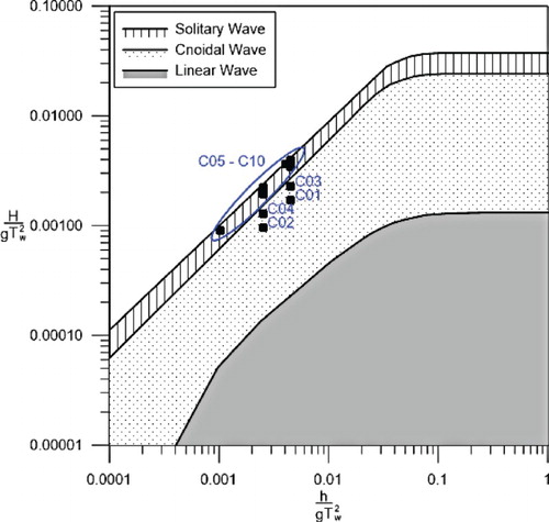
To describe the water waves mechanics (e.g. the flow velocities, orbital velocity, phase velocity, and pressure distribution), many mathematical solutions for the wave problem exist in the literature. One of the most common is Airy (1841) waves. Airy simplified the wave problem by conserving just the linear term into the governing equation (Laplace problem) and due to this, it is commonly called the linear wave theory. After the Airy wave, many other authors have included additional terms and different boundary conditions in the governing equation of the wave problem, to obtain more complex and nonlinear solutions. Each wave theory has limitations for his application and to know if one specific wave theory can be applied to a specific problem, many parameters must be previously defined. Le Mehaute (1976) proposes a graphical solution to determine where a wave theory can be applied as a function of wave mean height (H), wave period (), acceleration of gravity (g) and water depth (h).

To represent the oscillatory flow in the test channel, it was necessary to adopt two different theories: cnoidal (Cases 1 to 4) and solitary wave (Cases 5 to 10). Is important to say that in the case of the solitary wave the period is related to an apparent wave period defined has a proportion of the wavelength and the wave celerity.

The wave theories applied to each case were determined in accordance with the Le Mehaute (1976, ch. 15, p. 205) criterion; this author elaborated a graphical representation, in agreement with the valid range of each of them. Figure 2 presents an adaptation of the Le Mehaute (1976) graph, incorporating the simulated cases, which were previously described in Table 5.

Figure 2. Identification of the dominion of the wave theories applied to each of the oscillatory flow simulated cases, according to the Le Mehaute (1976) criterion.

REEF3D models are able to simulate wave propagation via the implementation of a numerical wave tank. To capture the surface movements, the level set method (Osher & Sethian, 1988) is applied. At the inlet, the waves are generated according to Mayer, Garapon, and Sørensen (1998), and are adapted to CFD models according to Jacobsen, Fuhrman, and Fredsøe (2012).

The cnoidal waves are imposed at the inlet according to the Korteweg and De Vries (1895) theory, while the solitary waves are imposed according to the Munk (1949) theory.

The time duration for each numerical simulation was adopted based on the recommendation of Kobayashi and Oda (1994).

The maximum scour obtained from the numerical simulation was made dimensionless with the pile diameter (S/D) and was expressed as a function of the Keulegan–Carpenter number with the purpose of enabling the comparison of these magnitudes with the laboratory test performed by Sumer et al. (1992) and Sumer and Fredsøe (2001).

3. Results

3.1. Model configuration - calibration test

3.1.1. Numerical behavior

The results obtained from the calibration process of the REEF3D numerical model to represent the scour around a cylindrical pile in a steady flow are presented in Figure 3. A comparison between the time series of the maximum dimensionless scour at the upstream region (Figure 3A) and at the downstream region (Figure 3B), obtained for each turbulence closure model employed, are shown.

Figure 3. S/D time series comparison: (a) upstream pile zone; (b) downstream pile zone.

The scour shown in Figure 3A, B have been obtained using a relaxation coefficient , with magnitudes equal to 1.0 and 0.8. This relaxation of the incipient sediment transport was only applied in a sub-area contained in the vicinity of the pile and whose width was equal to the channel width, while in the axial axis the distance was twice the pile diameter (2D), in both directions, upstream and downstream.

The REEF3D maximum scour obtained with the turbulent closure model is higher than the one determined by .

Likewise, the maximum scour obtained with the value of the relaxation coefficient, , equal to 0.8 is higher than the one determined when this coefficient is equal to 1, that is to say, when the incipient shear stress is applied just with the slope corrections proposed by Dey (2001).

The REEF3D simulation with = 0.8 is more or less equal to those reported by Baykal et al. (2015) for the upstream and downstream region (Figure 3). The REEF3D dimensionless scour S/D was 0.98 for the upstream region and 0.73 for the downstream region, while those values were 0.91 and 0.73 for Baykal et al. (2015). In general, the results obtained with REEF3D and models show similarities with the temporal behavior of S/D when they compare with the reported values by Baykal et al. (2015), being adequately represented both upstream and downstream zones of the pile. So the relaxation coefficient = 0.8, and the turbulent closure made the REEF3D a similar numerical model to the one of Baykal et al. (2015). In the next section the calibrated REEF3D is compared with experimental data.

3.1.2. Comparison with experimental data

The time series of pile scour evolution obtained from the REEF3D simulations of the experiment by Link (2006) are shown in Figure 4. Three different times are illustrated: (a) initial bed response (5 min after the beginning of the simulation) due to a constant discharge; (b) bed response after 2.1 h, or 10% of the total time of the simulation; and (c) bed response after 21 h, or the final time of the simulation.

Figure 4. Time series of scour around a pile obtained from REEF3D simulation. (a) 5 min after test initiation; (b) 2.1 h after test initiation; (c) 21 h after test initiation.

The results obtained from the comparison of the turbulent closures models and their ability to better represent the scour around a pile, turn out to be expected according to what was previously reported by Kato (1993), Baranya et al. (2012) and Hamidi and Siadatmousavi (2017), given that according to these authors, this turbulent closure is capable of producing greater turbulence in the upper region of the flow separation. This added to the bed shear stress that we are using (based on the turbulence, according to Equations (21(21) ) and (22(22) )) produces the results obtained and illustrated in Figure 3.

In the downstream, the results obtained are concordant with expectations, given that the RANS coupled with the turbulent closure model has a slight tendency to underestimate speeds near the bottom (Baranya et al., 2012) and in this way the TKE decreases and therefore the shear stress and consequent the sediment transport decrease as well.

Figure 4A shows that the initial scour starts at the sides of the pile. This bed response is due to the streamline contraction induced by the presence of the pile in the flow, which amplifies the bed shear stress, reaching a maximum over the incipient shear stress. The scour increased in time, both in area and depth (Figure 4B). Bed response at this time is developed around the pile.

Finally, Figure 4C shows the contour lines to the pile scour after 21 h of simulation, where the scour is fully developed and it is at equilibrium. The maximum scour depth is reached in front of the pile with a magnitude of 0.15 m (S/D = 0.75).

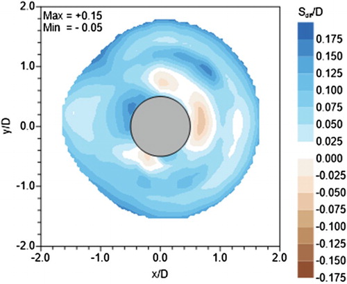
In general terms the results shown in Figure 4 are concordant with the time evolution of scour described previously by Melville and Chiew (1999) and Link et al. (2008b). Figure 5 presents the laboratory experiment of Link (2006) at 21 h and the REEF3D simulation for the same 21 h. It is shown that in both cases the maximum scour have the same value (0.15 m); however, this location differs slightly.

Figure 5. Scour contour lines comparison between experimental (Link, 2006) and numerical data, for 21 h of simulation.

The scour hole geometry determined by REEF3D has a larger area than that measured by Link (2006) in the laboratory and that is due to the relaxation coefficient area. However, both results (numerical and experimental) have similar magnitudes, with differences between –0.01 () to +0.03 m (), according to Figure 6. The mean value of the differences found between numerical and experimental data, has a magnitude of +0.01 meters (). That is, REEF3D showed a greater sensitivity to the bed response due to the forcing action of the uniform flow and, consequently, induced a greater scour.

Figure 6. Differences in the pile scour estimation between Link (2006) measurements and the numerical data obtained with REEF3D.

According to the results obtained, the REEF3D simulations were able to adequately reproduce the pile scour evolution and its maximum value, with a good agreement with the scour hole geometry.

3.2. Pile scour simulation for unsteady current and oscillatory flow

The results obtained for time series of maximum scour, in cm, for unsteady current, are presented in Figure 7A–E, with A and B being associated with a stepped distribution of discharges, C and D with a triangular distribution of discharges and, finally, E associated with the pulsating flow. In general terms, the numerical results fit well the experimental data, being in agreement both in the value of the maximum scour and geometric distribution of scour.

Figure 7. Comparison of the results obtained by REEF3D and those reported by Link et al. (2017), for the scour due unsteady flow. (a) Scour for hydrograph A; (b) scour for hydrograph B; (c) scour for hydrograph C; (d) scour for hydrograph D; (e) scour for hydrograph E.

The result in Figure 7A shows that the maximum scour around the pile has a geometrical agreement with the hydrograph employed to force the model. The maximum scour () increases if the discharge increase or remains constant. When the discharge begins to decrease, the scour remains constant. These results are comparable with those of Oliveto and Hager (2002), Chang et al.,  (2004), Gjunsburgs et al. (2010), Borghei, Kabiri-Samani, and Banihashem (2012), and Link et al. (2017), among others.

As can be seen in Figure 1A, the hydrograph has two steps before reaching its maximum and then, in the descent, also makes a step, symmetrical to the second step in the ascent, before stopping. In the ascent of the hydrograph the scour increases for two reasons; one reason is that the scour is increased as the discharge remains constant after reaching a step, because it has not yet reached its equilibrium scour. The other reason is that the scour is increased as the discharge is increasing from one step to the other. When the discharge begins to decrease (descent part of the hydrograph), the scour remains practically constant due to the fact the flow has not been capable to move the sediment into the scour hole.

In Figure 7B the scour does not reach an absolute maximum in the experiment or in the simulation final time. This is due to the hydrograph shape, in which the maximum discharge is reached 19 min after the test started and then remained constant for another 20 min, approximately. The time scale involved is shorter than that required for a permanent steady flow to reach the equilibrium scour.

The results in Figure 7C show the importance of both the maximum discharge and the time period in which the hydrograph acts, because the bed scour response increases until the discharge reaches its maximum value and remains constant during the whole remaining time of the test. In Figure 7D the hydrograph test also showed a constant behavior of the maximum scour, which is reached after the maximum discharge of the time series occurs.

The result obtained for the pulsating flow distribution (Figure 7E) indicates two steps in the maximum scour time evolution: the growing phase and the one in which the scour remains constant. At first glance, it is possible to see that the maximum scour increases with the discharge increment until reaching a maximum value around 6 cm, which is temporally concordant with the first peak of the hydrograph. During the discharge decrement phase, the maximum scour remains constant and increases only when the discharge returns to a crescent phase. According with the obtained results, both experimental and numerical, the maximum scour is expected to be a function of both the maximum discharge of the hydrograph and the time it acts over the bed.

One of the most relevant results found from the numerical model for each simulated hydrograph is the relationship between the maximum scour and the discharge behavior. In general terms the maximum scour induced by a specific discharge will increment if this discharge remains constant or increases; meanwhile if the discharge decreases, the maximum scour remains constant.

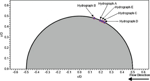
At the end of the pile scour simulation for each hydrograph considered, the maximum scour was located according to Figure 8, with azimuthal location of 62 for hydrograph D and 74 for hydrograph B.

Figure 8. Maximum scour location due to unsteady flow at the end of the experiment for each hydrograph simulated in REEF3D.

The results of the numerical simulation for the oscillatory flow shown in Figure 9 are presented compiling the information of Sumer et al. (1992) (experimental data and their empirical relationship) and Sumer and Fredsøe (2001). The dimensionless maximum scour (S/D) is presented as a function of the Keulegan–Carpenter number (KC), confirming, in every simulated case, a good fit both for the experimental data and the empirical equation.

Figure 9. Comparison between the dimensionless scour obtained from REEF3D and the results reported by Sumer et al. (1992) and Sumer and Fredsøe (2001).

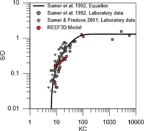
The dimensionless scour determined by the REEF3D model increases as a function of KC, in agreement with what was expected and previously described by Sumer et al. (1992) and Sumer and Fredsøe (2001), given that higher KC magnitudes imply more powerful horseshoe vortices and higher vortex shedding intensities. When comparing the numerical results with the empirical equation to predict the scour proposed by Sumer et al. (1992), even though the fit is coincident for both, the simulated data tends to underestimate the predicted values.

The obtained data from the numerical simulation were fitted to an exponential function in order to follow Sumer et al. (1992) proposed behavior for KC ≥ 6: (29)

To construct the previous equation, the shape of the function proposed by Sumer et al. (1992) was kept with the intention of making Equation (10(10) ) directly comparable with the proposed one but with a sole drawback. The Sumer et al. (1992) equation indicates that for KC tending to infinity, the maximum dimensionless scour (S/D) finds a limit of 1.3, which is concordant with the steady flow behavior. Nonetheless, Equation (10(10) ) with the numerical results shows the bound . This apparent increment in the maximum scour associated with the found fitting equation is due to the validity range, exclusively, since the numerical tests were only representing KC values less than 100, being unable to reflect the behavior associated with steady flow regime. If the fitting equation obtained by REEF3D is forced, so that the maximum dimensionless scour would converge to a steady flow solution, the following expression will be: (30)

When performing the forcing of the maximum dimensionless scour value with the numerical data to be fixed at 1.3, it can be obtained in practice using the equation presented by Sumer et al. (1992).

4. Discussion

The numerical simulation of the hydrodynamics around circular piles, presented in this article has been performed on the basis of a mesh that allows correct simulation of the behavior of the flow around the pile, being used in the vertical both for the case of uniform and impermanent flow, of the order of 15 cells (minimum 12 and maximum 17) it could be considered as a coarse grid to describe the flow. However, there are studies carried out by other authors who have used configurations similar to those used in this study.

Aghaee and Hakimzadeh (2010) carried out a numerical study of the three-dimensional flow field around piers, based on LES and RANS simulations, without considering the scour. In the case of the RANS simulation they used and 20 cells in the vertical axis. According to their conclusions, the flow predicted by the solution of the RANS equations with the closure model is similar to the flow observed in their experiment, and there was a good comparison with LES numerical simulations results as well.

Baranya et al. (2012) performed a numerical study using a three-dimensional numerical simulation using the RANS equations with the turbulent closure model , to evaluate the flow behavior around two configurations: a single pile and two piles. For this purpose, a nested grid system proposed by the authors was used. To define the vertical grid size, Baranya et al. (2012) performed a sensitivity analysis, which compared experimental results with numerical results considering a scheme with 12 cells and another with 20 cells. From this, it was concluded that the use of 12 layers vertically yielded an optimal resolution, since there was no significant change in the flow pattern when employing a finer resolution of 20 layers.

Baranya et al. (2012) concluded that, in the case of single pier, the RANS equations with turbulent closure agree adequately with laboratory observations in the area upstream of the pile. However, in the downstream a slight underestimation of the velocities near the bed can be observed.

Similar conditions for numerical simulation (RANS + ) were applied by Mohamed (2012), considering scour at two submerged-emerged tandem cylindrical piers. For the vertical flow definition they used 14 cells, and achieved good agreement of their numerical results with experimental data, when comparing the scour around the piles.

Thanh, Chung, & Nghien (2014) studied the scour around a rectangular pile, solved under a scheme of finite differences of the RANS with the turbulent closure model, using a definition in the vertical of 12 cells. They compared their results with experimental scour data, finding a good relationship between measurements and numerical simulations, both in maximum magnitude and location.

Afzal et al. (2015) applied the REEF3D numerical model with the turbulent closure model, to study in a three-dimensional way the scour around a pile from the action of waves and currents. In the configuration, the authors used 12 vertical cells to describe the hydrodynamics due to currents and 11 cells in the case of the oscillatory flow induced by the waves. Their results when compared with experimental data showed good agreement in the case of currents.

Recently, Hamidi & Siadatmousavi (2017) performed numerical simulation of scour and hydrodynamics by applying RANS with both the turbulent closure and , for different pile arrangements, and compared their numerical results with experimental ones. The authors configured the model to describe the vertical one by means of the use of 12 cells, which is comparable with the configuration that the present authors have adopted.

It can be seen that our configuration of the numerical model is equivalent to that presented by Aghaee & Hakimzadeh (2010), Baranya et al. (2012), Mohamed (2012), Thanh et al. (2014), Afzal et al. (2015) and Hamidi & Siadatmousavi (2017), so it is expected that the flow around the pile was well simulated.

Bihs, Kamath, Chella, Aggarwal, & Arntsen (2016) used REEF3D to simulate the flow around a circular pile and also a rectangular abutment due to waves. The general performance of the numerical model was tested, using different grid sizes. In the case of piles exposed to waves, a grid resolution study was carried out, using 10, 20, 40 and 80 cells in the vertical axis to describe the hydrodynamics. According to their results, a grid with 40 cells in the vertical axis is enough to describe the waves and the hydrodynamics induced by it.

Baykal et al. (2017), as a continuation of the Roulund et al. (2005) study, numerically studied the scour and the backfilling processes around a mono pile. The flow is defined using a solution of RANS equations with as a turbulent closure model. The vertical axis uses 14 cells for the simulated cases with rigid bed and 16 cells for the live-bed simulated cases.

In the wave test simulated in this research, 100 cells were used in the vertical for cases C01 to C08, and 200 cells for cases C09 and C10. If these vertical resolutions are compared with the configuration adopted by Bihs et al. (2016) and Baykal et al. (2017), a better description of the hydrodynamics induced by waves around cylindrical piles can be expected from our numerical simulation.

According to the calibration test, a relaxation coefficient equal to 0.8 was necessary to reproduce adequately the scour. acting as a weighting coefficient of the incipient shear stress, increases the mobility of the sediment in order to improve the comparison among the scour simulations and experimental measurements or field data. From a physical point of view, the relaxation coefficient employed in the numerical model does not directly represent an additional mechanism for sediment transport and/or inter-granular interactions that could favor sediment mobility. Conversely, it allows regulation of the sedimentation dynamics that develop around the pile, a situation that has not been properly described yet in the literature.

The dynamics of the sediment transport near an obstruction to the flow was approached by Hager and Oliveto (2002) and applied by Oliveto and Hager (2002), who assign the incipient motion as a function of the densitometric Froude number. According to the incipient criterion of Hager and Oliveto (2002), critical shear stress under the effect of a pile is less than the Shields criterion and based on this, the relaxation coefficient indicated by Bihs (2011), and employed in this numerical simulation, acquires a physical meaning. That is to say, the relaxation coefficient tries to reproduce the sediment transport behavior near the pile.

The use of a relaxation coefficient in the calculation of sediment transport under the effect of the pile led to results that were comparable with the experimental data, both for unsteady flow and oscillatory flow. However, at the same time, it constrains considerably the direct applicability of the numerical tool in situations that have not been studied in the laboratory or in the field, because there is not a background that would allow calibrating or verifying the magnitude of such a factor.

Wang and Jia (1999) examined the importance of including additional flow effects on sediment transport estimation when the scour phenomena are included. These authors propose empirical functions to alter shear stress in an empirical sediment transport model to account the effects produced by the mean flow, down flow, vortices and turbulence intensity.

Cheng, Koken, and Constantinescu (2017) recognized that the coherent turbulent structures that develop near the bed have an effect on the incipient motion and must be incorporated into the RANS by means of modifications of this.

In order to overcome the limitations mentioned by Wang and Jia (1999) and Cheng et al. (2017) when a simplified description of the mechanims of sediment motion is used, a relaxation coefficient was employed to improve the calculation of the sediment transport under the effect of a pile.

In the unsteady flow case, the obtained results were concordant with the technical discussions previously given by Oliveto and Hager (2002), Chang et al.,  (2004), Borghei et al. (2012), Gjunsburgs et al. (2010) and Link et al. (2017), among others, detecting two relevant aspects: the maximum discharge magnitude and the time in which this acts.

In the unsteady current scour computation, maximum scour is reached instantly with the maximum discharge and the scour will only increase further if the discharge remains constant or increases, whereas it will stabilize if the discharge decreases. This situation shows the importance of the time scale in the morphodynamic equilibrium process, since maintaining the maximum discharge constant could be similar to a steady flow, a case which will require prolonged action to reach the maximum scour.

The scour associated with an oscillatory flow has been determined by applying the sediment transport equation developed by Meyer-Peter and Müller (1948), although this is for steady flow. However, its applicability to simulate the sediment transport associated with oscillatory flow (waves) is based on Ribberink (1998), who proposed a bed load transport equation with similar characteristics to the Meyer-Peter and Müller (1948) formula, but increasing their constant parameters to represent the effect of the oscillatory flow.

In this study, the Meyer-Peter and Müller (1948) equation was able to represent adequately the expected scour when this was compared with the results of Sumer et al. (1992).

5. Conclusions

The relaxation coefficient of sediment critical shear stress proposed by Bihs (2011) is fundamental for the REEF3D numerical model, and it must be selected by comparison with experimental data, to adequately represent the bed response in the surroundings of flow obstructions. The relaxation coefficient was 0.8 for steady, unsteady and oscillatory flow and it must be applied in a sub-area contained in the vicinity of the pile with width equal to the channel width, while in the axial axis the distance was twice the diameter of the pile, in both directions, upstream and downstream.

The REEF3D model was calibrated by comparison with numerical results of other authors (Baykal et al., 2015) and laboratory data (Link, 2006), both under steady flow.

When the relaxation coefficient was applied to unsteady flow and oscillatory flow, the numerical modeled results adjusted correctly to the experimental data. In particular, concerning the obtained results for unsteady flow, the numerical model with the adopted configuration was capable of representing the morphodynamic behavior of the scour relative to its maximum value, being concordant, both in the temporal development and the prolonged action effects of the maximum discharge of the hydrograph.

The temporal behavior of the pile scour obtained from the numerical simulation was well represented in general terms, being able to reproduce the expected behavior according to Borghei et al. (2012); Chang et al.,  (2004); Gjunsburgs et al. (2010); Link et al. (2017); Oliveto and Hager (2002). The numerical scour can overestimate (tests A, C and E) or underestimate (tests B and D) the experimental data, however the differences are small.

In the oscillatory flow case, the obtained results fitted well with the experimental data published by Sumer et al. (1992) and Sumer and Fredsøe (2001), representing the same phenomenon, adjusting well the numerical data to the predictive equations available in the literature.

When the numerical results for the dimensionless pile scour due to oscillatory flow are compiled according to the Keulegan–Carpenter number, they are adjusted in the same form as Sumer et al. (1992). This is an indicator that the numerical model could forecast the pile scour in concordance with the experimental data.

Use of the Meyer-Peter and Müller (1948) formula allowed representation of sediment transport associated with both unsteady and oscillatory flow, despite its semi-empirical foundation being based on cases of unidimensional steady flow.

According to the results obtained here and in the cited studies, the authors consider necessary to continue with the study of incipient transport of sediments near piles or other flow obstacles, to define the threshold value or incorporate the turbulent effects induced by the obstacle over the sediment motion estimation.

ORCID

Matias Quezada http://orcid.org/0000-0002-0596-9529

Aldo Tamburrino http://orcid.org/0000-0001-5406-370X

Y. Niño http://orcid.org/0000-0002-0108-2656

Additional information

Funding

The authors acknowledge support from the Civil Engineering Department, Universidad de Chile and the PhD program in Fluid-dynamics. The first author acknowledges financial support from the CONICYT doctoral fellowship [21140091].

References

- Afzal, M. S., Bihs, H., Kamath, A., & Arntsen Ø, A. (2015). Three-dimensional numerical modeling of pier scour under current and waves using level-set method. Journal of Offshore Mechanics and Arctic Engineering, 137(3): 032001.
- Aghaee, Y., & Hakimzadeh, H. (2010). Three dimensional numerical modeling of flow around bridge piers using LES and RANS. In Dittrich, Koll, Aberle Geisenhainer (Eds.), River Flow, (pp. 211–218). Karlsruhe: Bundesanstalt für Wasserbau, Germany.
- Ahmad, N., Bihs, H., Kamath, A., & Arntsen Ø, A. (2015). Three-dimensional CFD modeling of wave scour around side-by-side and triangular arrangement of piles with REEF3D. Procedia Engineering, 116, 683–690. doi: 10.1016/j.proeng.2015.08.355
- Airy, G. B. (1841). Tides and waves. Encyclopedia Metropolitana,, 192, 241–396.
- Altomare, C., Crespo, A. J., Domínguez, J. M., Gómez-Gesteira, M., Suzuki, T., & Verwaest, T. (2015). Applicability of smoothed particle hydrodynamics for estimation of sea wave impact on coastal structures. Coastal Engineering, 96, 1–12. doi: 10.1016/j.coastaleng.2014.11.001
- Baker, C. (1979). The laminar horseshoe vortex. Journal of Fluid Mechanics, 95(02), 347–367. doi: 10.1017/S0022112079001506
- Baker, C. (1980). The turbulent horseshoe vortex. Journal of Wind Engineering and Industrial Aerodynamics, 6(12), 9–23. doi: 10.1016/0167-6105(80)90018-5
- Baranya, S., Olsen, N., Stoesser, T., & Sturm, T. (2012). Three-dimensional rans modeling of flow around circular piers using nested grids. Engineering Applications of Computational Fluid Mechanics, 6(4), 648–662. doi: 10.1080/19942060.2012.11015449
- Baykal, C., Sumer, B. M., Fuhrman, D. R., Jacobsen, N. G., & Fredsøe, J. (2015). Numerical investigation of flow and scour around a vertical circular cylinder. Philosophical Transactions of the Royal Society of London A: Mathematical, Physical and Engineering Sciences, 373(2033), 20140104.
- Baykal, C., Sumer, B. M., Fuhrman, D. R., Jacobsen, N. G., & Fredsøe, J. (2017). Numerical simulation of scour and backfilling processes around a circular pile in waves. Coastal Engineering, 122, 87–107. doi: 10.1016/j.coastaleng.2017.01.004
- Berthelsen, P. A. (2004). A decomposed immersed interface method for variable coefficient elliptic equations with non-smooth and discontinuous solutions. Journal of Computational Physics, 197(1), 364–386. doi: 10.1016/j.jcp.2003.12.003
- Bihs, H. (2011). Three-dimensional numerical modeling of local scouring in open channel flow. (PhD thesis), Norwegian University of Science and Technology, Trondheim, Norway.
- Bihs, H., Kamath, A., Chella, M. A., Aggarwal, A., & Arntsen Ø, A. (2016). A new level set numerical wave tank with improved density interpolation for complex wave hydrodynamics. Computers & Fluids, 140, 191–208. doi: 10.1016/j.compfluid.2016.09.012
- Borghei, S. M., Kabiri-Samani, A., & Banihashem, S. A. (2012). Influence of unsteady flow hydrograph shape on local scouring around bridge pier. In Proceedings of the Institution of Civil Engineers-Water Management, 165, 473–480. doi: 10.1680/wama.11.00020
- Breusers, H., Nicollet, G., & Shen, H. (1977). Local scour around cylindrical piers. Journal of Hydraulic Research, 15(3), 211–252. doi: 10.1080/00221687709499645
- Brevis, W., & García-Villalba, M. (2014). Experimental and large eddy simulation study of the flow developed by a sequence of lateral obstacles. Environmental Fluid Mechanics, 14(4), 873–893. doi: 10.1007/s10652-013-9328-x
- Burkow, M. (2010). Numerische simulation stromungsbedingten sedimenttransports und der entstehenden gerinnebettformen. (Master's thesis). Bonn, Germany: Mathematisch-Naturwissenschaftlichen Fakultat der Rheinischen Friedrich-Wilhelms-Universitat Bonn.
- Chang, W.-Y., Lai, J.-S., & Yen, C.-L. (2004). Evolution of scour depth at circular bridge piers. Journal of Hydraulic Engineering, 130(9), 905–913. doi: 10.1061/(ASCE)0733-9429(2004)130:9(905)
- Chau, K., & Jiang, Y. (2001). 3D numerical model for Pearl River estuary. Journal of Hydraulic Engineering, 127(1), 72–82. doi: 10.1061/(ASCE)0733-9429(2001)127:1(72)
- K., Chau ,, & Jiang, Y. (2004). A three-dimensional pollutant transport model in orthogonal curvilinear and sigma coordinate system for Pearl river estuary. International Journal of Environment and Pollution, 21(2), 188–198. doi: 10.1504/IJEP.2004.004185
- Cheng, Z., Koken, M., & Constantinescu, G. (2017). Approximate methodology to account for effects of coherent structures on sediment entrainment in RANS simulations with a movable bed and applications to pier scour. Advances in Water Resources. doi: 10.1016/j.advwatres.2017.05.019.
- Chorin, A. J. (1968). Numerical solution of the Navier-Stokes equations. Mathematics of Computation, 22(104), 745–762. doi: 10.1090/S0025-5718-1968-0242392-2
- Dalrymple, R., & Rogers, B. (2006). Numerical modeling of water waves with the SPH method. Coastal Engineering, 53(2), 141–147. doi: 10.1016/j.coastaleng.2005.10.004
- Das, S., Das, R., & Mazumdar, A. (2013). Circulation characteristics of horseshoe vortex in scour region around circular piers. Water Science and Engineering, 6(1), 59–77.
- Davies, D. R., Wilson, C. R., & Kramer, S. C. (2011). Fluidity, A fully unstructured anisotropic adaptive mesh computational modeling framework for geodynamics. Geochemistry, Geophysics, Geosystems, 12(6) doi: 10.1029/2011GC003551
- Dey, S. (2001). Experimental studies on incipient motion of sediment particles on generalized sloping fluvial beds. Journal of Sediment Research, 16(3), 391–398.
- Dey, S., & Raikar, R. V. (2007). Characteristics of horseshoe vortex in developing scour holes at piers. Journal of Hydraulic Engineering, 133(4), 399–413. doi: 10.1061/(ASCE)0733-9429(2007)133:4(399)
- Diab, R., Link, O., & Zanke, U. (2010). Geometry of developing and equilibrium scour holes at bridge piers in gravel. Canadian Journal of Civil Engineering, 37(4), 544–552. doi: 10.1139/L09-176
- Doolan, C. (2010). Large eddy simulation of the near wake of a circular cylinder at sub-critical Reynolds number. Engineering Applications of Computational Fluid Mechanics, 4(4), 496–510. doi: 10.1080/19942060.2010.11015336
- Engelund, F., & Fredsøe, J. (1976). A sediment transport model for straight alluvial channels. Nordic Hydrology, 7(5), 293–306.
- Enright, D., Fedkiw, R., Ferziger, J., & Mitchell, I. (2002). A hybrid particle level set method for improved interface capturing. Journal of Computational physics, 183(1), 83–116. doi: 10.1006/jcph.2002.7166
- Escauriaza, C., & Sotiropoulos, F. (2011). Lagrangian model of bed-load transport in turbulent junction flows. Journal of Fluid Mechanics, 666, 36–76. doi: 10.1017/S0022112010004192
- Exner, F. M. (1925). Uber die wechselwirkung zwischen wasser und geschiebe in fülssen. Akad. Wiss. Wien Math. Naturwiss. Klasse, 134(2), 165–204.
- Fourtakas, G., & Rogers, B. (2016). Modelling multi-phase liquid-sediment scour and resuspension induced by rapid flows using smoothed particle hydrodynamics (sph) accelerated with a graphics processing unit (gpu). Advances in Water Resources, 92, 186–199. doi: 10.1016/j.advwatres.2016.04.009
- Fredsøe, J., & Deigaard, R. (1992). Mechanics of coastal sediment transport. Advanced Series on Ocean Engineering, Volume 3. World Scientific. Jurong East, Singapore.
- Gjunsburgs, B., Jaudzems, G., & Govša, J. (2010). Hydrograph shape impact on the scour development with time at engineering structures in river flow. Scientific Journal of Riga Technical, University Construction Science, 11, 6–12.
- Greifzu, F., Kratzsch, C., Forgber, T., Lindner, F., & Schwarze, R. (2016). Assessment of particle-tracking models for dispersed particle-laden flows implemented in OPENFOAM and ANSYS fluent. Engineering Applications of Computational Fluid Mechanics, 10(1), 30–43. doi: 10.1080/19942060.2015.1104266
- Hager, W. H., & Oliveto, G. (2002). Shields' entrainment criterion in bridge hydraulics. Journal of Hydraulic Engineering, 128(5), 538–542. doi: 10.1061/(ASCE)0733-9429(2002)128:5(538)
- Hamidi, A., & Siadatmousavi, S. M. (2017). Numerical simulation of scour and flow field for different arrangements of two piers using SSIIM model. Ain Shams Engineering Journal. doi: 10.1016/j.asej.2017.03.012.
- Haque, M. N., Katsuchi, H., Yamada, H., & Nishio, M. (2016). Flow field analysis of a pentagonal-shaped bridge deck by unsteady RANS. Engineering Applications of Computational Fluid Mechanics, 10(1), 1–16. doi: 10.1080/19942060.2015.1099569
- Hirt, C., & Cook, J. (1972). Calculating three-dimensional flows around structures and over rough terrain. Journal of Computational Physics, 10(2), 324–340. doi: 10.1016/0021-9991(72)90070-8
- Issa, R. I. (1986). Solution of the implicitly discretised fluid flow equations by operator-splitting. Journal of Computational Physics, 62(1), 40–65. doi: 10.1016/0021-9991(86)90099-9
- Jacobs, C. T., Goldin, T. J., Collins, G. S., Piggott, M. D., Kramer, S. C., Melosh, H. J., Wilson, C. R., & P. A. Allison , (2015). An improved quantitative measure of the tendency for volcanic ash plumes to form in water, implications for the deposition of marine ash beds. Journal of Volcanology and Geothermal Research, 290, 114–124. doi: 10.1016/j.jvolgeores.2014.10.015
- Jacobsen, N. G., Fuhrman, D. R., & FredsØe, J. (2012). A wave generation toolbox for the open-source cfd library, Openfoam. International Journal for Numerical Methods in Fluids, 70(9), 1073–1088. doi: 10.1002/fld.2726
- Jiang, G.-S., & Shu, C.-W. (1996). Efficient implementation of weighted eno schemes. Journal of Computational Physics, 126(1), 202–228. doi: 10.1006/jcph.1996.0130
- Kato, M. (1993). The modelling of turbulent flow around stationary and vibrating square cylinders. Turbulent Shear Flow, 1, 10–4.
- Keutner, C. (1932). Stromungsvorgange an strompfeilern von verschiedenen grundrissformen und ihre einwirkung auf die flussohle. Die Bautechnik, 10(12), 161–170.
- Kobayashi, T. (1992). Three-dimensional analysis of the flow around a vertical cylinder on a scoured seabed. Coastal Engineering Proceedings, 3(99), 3482–3495.
- Kobayashi, T., & Oda, K. (1994). Experimental study on developing process of local scour around a vertical cylinder. Coastal Engineering Proceedings, 1(24), 1284–1297.
- Komar, P. D., & Miller, M. C. (1975). On the comparison between the threshold of sediment motion under waves and unidirectional currents with a discussion of the practical evaluation of the threshold, Reply. Journal of Sedimentary Research, 45(1), 362–367.
- Korteweg, D. J., & De Vries, G. (1895). On the change of form of long waves advancing in a rectangular canal, and on a new type of long stationary waves. The London, Edinburgh, and Dublin Philosophical Magazine and Journal of Science, 39(240), 422–443. doi: 10.1080/14786449508620739
- Kothyari, U. C., Garde, R. C. J., & Ranga Raju, K. G. (1992). Temporal variation of scour around circular bridge piers. Journal of Hydraulic Engineering, 118(8), 1091–1106. doi: 10.1061/(ASCE)0733-9429(1992)118:8(1091)
- Launder, B., & Sharma, B. (1974). Application of the energy-dissipation model of turbulence to the calculation of flow near a spinning disc. Letters in Heat and Mass Transfer, 1, 1(12), 131–137.
- Launder, B. E., & Spalding, D. B. (1974). The numerical computation of turbulent flows. Computer Methods in Applied Mechanics and Engineering, 3(2), 269–289. doi: 10.1016/0045-7825(74)90029-2
- Laursen, E. M., & Toch, A. (1956). Scour around bridge piers and abutments, Volume 4. Iowa Highway Research Board Ames, IA.
- Le, Mehaute B. (1976). An introduction to hydrodynamics and water waves. Springer Science & Business Media, Pasadena, California.
- Leveque, R. J., & Li, Z. (1994). The immersed interface method for elliptic equations with discontinuous coefficients and singular sources. SIAM Journal on Numerical Analysis, 31(4), 1019–1044. doi: 10.1137/0731054
- Link, O. (2006). Untersuchung der Kolkung an einem schlanken zylindrischen Pfeiler in sandigem Boden. (PhD thesis) Inst. für Wasserbau u. Wasserwirtschaft.
- Link, O., Castillo, C., Pizarro, A., Rojas, A., Ettmer, B., Escauriaza, C., & Manfreda, S. (2017). A model of bridge pier scour during flood waves. Journal of Hydraulic Research, 55(3), 310–323. doi: 10.1080/00221686.2016.1252802
- Link, O., Gobert, C., Manhart, M., & Zanke, U. (2008a). Effect of the horseshoe vortex system on the geometry of a developing scour hole at a cylinder. In 4th International Conference on Scour and Erosion. Surugadai Memorial Hall, Chuo University, Tokyo, Japan, 162–168.
- Link, O., Pfleger, F., & Zanke, U. (2008b). Characteristics of developing scour-holes at a sand-embedded cylinder. International Journal of Sediment Research, 23(3), 258–266. doi: 10.1016/S1001-6279(08)60023-2
- Liu, X., & García, M. H. (2008). Three-dimensional numerical model with free water surface and mesh deformation for local sediment scour. Journal of Waterway, Port, Coastal, and Ocean Engineering. 134:203–217. doi: 10.1061/(ASCE)0733-950X(2008)134:4(203)
- Mayer, S., Garapon, A., & Sørensen, L. (1998). A fractional step method for unsteady free-surface flow with applications to non-linear wave dynamics. International Journal for Numerical Methods in Fluids, 28(2), 293–315. doi: 10.1002/(SICI)1097-0363(19980815)28:2<293::AID-FLD719>3.0.CO;2-1
- Melville, B. (2008). The physics of local scour at bridge piers. In Fourth International Conference on Scour and Erosion. Tokyo, Japan, 28–38.
- Melville, B. W. (1975). Local scour at bridge sites. (PhD thesis), University of Auckland, School of Engineering.
- Melville, B. W., & Chiew, Y.-M. (1999). Time scale for local scour at bridge piers. Journal of Hydraulic Engineering, 125(1), 59–65. doi: 10.1061/(ASCE)0733-9429(1999)125:1(59)
- Menter, F. R. (1994). Two-equation eddy-viscosity turbulence models for engineering applications. AIAA journal, 32(8), 1598–1605. doi: 10.2514/3.12149
- Meyer-Peter, E., & Müller, R. (1948). Formulas for bed-load transport. In Proceedings, Second Congress IAHR, Stockholm, Sweden, 1948.
- Mia, M. F., & Nago, H. (2003). Closure to design method of time dependent local scour at circular bridge pier. Journal of Hydraulic Engineering, 129, 420–427. doi: 10.1061/(ASCE)0733-9429(2003)129:6(420)
- Mohamed, H. I. (2012). Numerical simulation of flow and local scour at two submerged emergent tandem cylindrical piers. Journal of Engineering Sciences, 41(1), 1–19.
- Munk, W. H. (1949). The solitary wave theory and its application to surf problems. Annals of the New York Academy of Sciences, 51(1), 376–424. doi: 10.1111/j.1749-6632.1949.tb27281.x
- Oishi, Y., Piggott, M. D., Maeda, T., Kramer, S. C., Collins, G. S., Tsushima, H., & Furumura, T. (2013). Three-dimensional tsunami propagation simulations using an unstructured mesh finite element model. Journal of Geophysical Research, Solid Earth, 118(6), 2998–3018. doi: 10.1002/jgrb.50225
- Oliveto, G., & Hager, W. H. (2002). Temporal evolution of clear-water pier and abutment scour. Journal of Hydraulic Engineering, 128(9), 811–820. doi: 10.1061/(ASCE)0733-9429(2002)128:9(811)
- Olsen, N. R., & Kjellesvig, H. M. (1998). Three-dimensional numerical flow modeling for estimation of maximum local scour depth. Journal of Hydraulic Research, 36(4), 579–590. doi: 10.1080/00221689809498610
- Olsen, N. R., & Melaaen, M. C. (1993). Three-dimensional calculation of scour around cylinders. Journal of Hydraulic Engineering, 119(9), 1048–1054. doi: 10.1061/(ASCE)0733-9429(1993)119:9(1048)
- Osher, S., & Sethian, J. A. (1988). Fronts propagating with curvature-dependent speed, algorithms based on Hamilton-Jacobi formulations. Journal of Computational Physics, 79(1), 12–49. doi: 10.1016/0021-9991(88)90002-2
- Özkan, F., Wenka, A., Hansjosten, E., P., Pfeifer ,, B., Kraushaar-Czarnetzki , (2016). Numerical investigation of interfacial mass transfer in two phase flows using the VOF method. Engineering Applications of Computational Fluid Mechanics, 10(1), 100–110. doi: 10.1080/19942060.2015.1061555
- Paola, C., & Voller, V. (2005). A generalized exner equation for sediment mass balance. Journal of Geophysical Research: Earth Surface, 110(F4), F04014. doi: 10.1029/2004JF000274
- Patankar, S. V., & Spalding, D. B. (1972). A calculation procedure for heat, mass and momentum transfer in three-dimensional parabolic flows. International journal of heat and mass transfer, 15(10), 1787–1806. doi: 10.1016/0017-9310(72)90054-3
- Posey, C. (1949). Why bridges fail in floods. Civil Engineering, 19, 42.
- Reynolds, O. (1895). On the dynamical theory of incompressible viscous fluids and the determination of the criterion. Philosophical Transactions of the Royal Society of London. A, 186, 123–164. doi: 10.1098/rsta.1895.0004
- Ribberink, J. S. (1998). Bed-load transport for steady flows and unsteady oscillatory flows. Coastal Engineering, 34(1), 59–82. doi: 10.1016/S0378-3839(98)00013-1
- Roper, A., Schneider, V., & Shen, H. (1967). Analytical approach to local scour. In Proceedings of the 12th IAHR Congress, Ft. Collins, 3, 151–161.
- Roulund, A., Sumer, B. M., Fredsøe, J., & Michelsen, J. (2005). Numerical and experimental investigation of flow and scour around a circular pile. Journal of Fluid Mechanics, 534, 351–401. doi: 10.1017/S0022112005004507
- Saghatchi, R., Ghazanfarian, J., & Gorji-Bandpy, M. (2014). Numerical simulation of water-entry and sedimentation of an elliptic cylinder using smoothed-particle hydrodynamics method. Journal of Offshore Mechanics and Arctic Engineering, 136(3), 031801. doi: 10.1115/1.4026844
- Saud, M. (2013). 3D numerical modelling of sediment transport under current and waves. (MSc-Thesis) Coastal and Marine Engineering and Management, Norwegian University of Science and Technology.
- Shields, A. (1936). Application of similarity principles and turbulence research to bed-load movement. (PhD thesis), Technical University Berlin, Preussischen Versuchsanstalt für Wasserbau.
- Sumer, M. B. (2007). Mathematical modelling of scour: A review. Journal of Hydraulic Research, 45(6), 723–735. doi: 10.1080/00221686.2007.9521811
- Sumer, B. M., Christiansen, N., & Fredsøe, J. (1997). The horseshoe vortex and vortex shedding around a vertical wall-mounted cylinder exposed to waves. Journal of Fluid Mechanics, 332, 41–70. doi: 10.1017/S0022112096003898
- Sumer, B. M., & Fredsøe, J. (2001). Wave scour around a large vertical circular cylinder. Journal of Waterway, Port, Coastal, and Ocean Engineering, 127(3), 125–134. doi: 10.1061/(ASCE)0733-950X(2001)127:3(125)
- Sumer, B. M., & Fredsøe, J. (2002). The mechanics of scour in the marine environment. Jurong East, Singapore: World Scientific Publishing Co. Pte. Ltd.
- Sumer, B. M., Fredsøe, J., & Christiansen, N. (1992). Scour around vertical pile in waves. Journal of Waterway, Port, Coastal, and Ocean Engineering, 118(1), 15–31. doi: 10.1061/(ASCE)0733-950X(1992)118:1(15)
- Sumer, B. M., Petersen, T. U., Locatelli, L., Fredsøe, J., Musumeci, R. E., & Foti, E. (2013). Backfilling of a scour hole around a pile in waves and current. Journal of Waterway, Port, Coastal, and Ocean Engineering, 139(1), 9–23. doi: 10.1061/(ASCE)WW.1943-5460.0000161
- Thanh, N. V., Chung, D. H., & Nghien, T. D. (2014). Prediction of the local scour at the bridge square pier using a 3D numerical model. Open Journal of Applied Sciences, 4(02), 34.
- Tison, L. (1940). Erosion autour de piles de ponts en riviere. In Annales des Travaux publics de Belgique, 41, 813–817.
- Trewhela, T., C., Ihle ,, Tamburrino, A. (2014). Numerical simulations of comminution slurries over complex topographies: Putting together CFD and pipeline integrity. Minerals Engineering, 63, 139–148. doi: 10.1016/j.mineng.2014.03.005
- Tseng, Y.-H., & Ferziger, J. H. (2003). A ghost-cell immersed boundary method for flow in complex geometry. Journal of Computational Physics, 192(2), 593–623. doi: 10.1016/j.jcp.2003.07.024
- Ulloa, H., Winters, K., & delaFuente, A. (2015). Degeneration of internal Kelvin waves in a continuous two-layer stratification. Journal of Fluid Mechanics, 777, 68–96. doi: 10.1017/jfm.2015.311
- Unger, J., & Hager, W. H. (2007). Down-flow and horseshoe vortex characteristics of sediment embedded bridge piers. Experiments in Fluids, 42(1), 1–19. doi: 10.1007/s00348-006-0209-7
- VanRijn, L. C. (1984). Sediment transport, Part II: Suspend load transport. Journal of Hydraulic Engineering, 110(11), 1613–1641. doi: 10.1061/(ASCE)0733-9429(1984)110:11(1613)
- Van Rijn, L. C. (1984a). Sediment transport, Part I: Bed load transport. Journal of Hydraulic Engineering, 110(10), 1431–1456. doi: 10.1061/(ASCE)0733-9429(1984)110:10(1431)
- Wang, S., & Jia, Y. (1999). Computational simulations of local scour at bridge crossings–capabilities and limitations. In International Water Resources Conference on Water Resources into the New Millennium: Past Accomplishments and New Challenges ASCE, Seattle, pp. 8–12.
- Wilcox, D. C. (1998). Turbulence modeling for CFD, Volume 2. DCW industries La Canada, CA.
- C., Wu ,, Chau, K. (2006). Mathematical model of water quality rehabilitation with rainwater utilisation: a case study at Haigang. International Journal of Environment and Pollution, 24(34), 534–545. doi: 10.1504/IJEP.2006.011227
- Xie, J., & Yee-Chung, J. (2016). Parameter determination for the Cross rheology equation and its application to modeling non-Newtonian flows using the WC-MPS method. Engineering Applications of Computational Fluid Mechanics, 6(1), 111–129. doi: 10.1080/19942060.2015.1104267
- Yalin, M. S. (1972). Mechanics of Sediment Transport. New York: Pergamon Press.
- Yuhi, M., Ishida, B., & Umeda, S. (2000). A numerical study of three-dimensional flow fields around a vertical cylinder mounted on a bed. Coastal Structures Proceedings, 2, 783–792.