Numerical prediction of shock/boundary-layer interactions at high Mach numbers using a modified Spalart–Allmaras model

ABSTRACT

The Reynolds-averaged Navier–Stokes equations with one-equation turbulence models are used to simulate the flow field past a cone–flare geometry in the Mach number range from 5 to 8 with emphasis on the interaction region of the flare shock with the upstream boundary layer. A model based on the physics of shock unsteadiness is used to correct the standard Spalart–Allmaras turbulence model to improve the prediction of the extent of the separation bubble arising from the shock/turbulent boundary-layer interaction and its accompanying peak pressure and aerothermal loads on the surface. The computed results are validated against the experimental data. The limitations of the shock-unsteadiness model and the extent of the improvement in predicting the heat flux are discussed.

KEYWORDS:

• High speed flows
• shock wave
• turbulent boundary layer
• shock unsteadiness
• separation bubble
• turbulence modeling

View correction statement:

Corrigendum

Nomenclature

	=	shock-unsteadiness damping parameter
	=	model parameter
	=	skin-friction coefficient
k	=	turbulent kinetic energy
	=	upstream Mach number normal to shock
	=	production of turbulent eddy viscosity
s	=	streamline distance along wall measured from cone tip
	=	mean dilatation
θ	=	deflection angle
μ	=	absolute molecular viscosity
ν	=	kinematic molecular viscosity
	=	turbulent kinematic viscosity
	=	mean density
	=	turbulence field variable
ε	=	turbulent dissipation rate

Subscripts

0	=	upstream of interaction
n	=	normal to shock wave
w	=	wall condition
∞	=	free-stream conditions

1. Introduction

Hypersonic vehicle design involves aerothermodynamics analysis due to the high temperatures generated across different shock waves and viscous dissipation occurring on its surface. The shock waves generated at high Mach numbers are inclined to, and remain close to, the vehicle surface, and invoke complex physics when they interact with the boundary layer developed on the walls to form a shock/boundary-layer interaction. The shock–shock and shock/boundary-layer interactions are more prominent in hypersonic flows. The high pressure and heating loads generated from these interactions play a significant role in the control surface effectiveness and structural integrity of hypersonic vehicles (Bose et al., 2013). The cone–flare configuration finds its applications in hypersonic aerospace vehicles. It consists of a cone of small apex angle followed by a flare, inclined at a larger angle. At hypersonic flows, a shock generated at the corner of the cone–flare junction is inclined very close to the boundary layer developed on the flare surface. The oblique shock at the cone–flare junction interacts with the upstream turbulent boundary layer. The strength of the shock is directly proportional to the pressure ratio across the shock, which in turn depends on the upstream Mach number normal to the shock. If the shock wave is strong enough to cause separation of the boundary layer, an unsteady interaction region is generated at the junction. The shock-wave/turbulent boundary-layer interaction in the hypersonic flow regime is characterized by localized regions of peak pressure, skin friction, and heat-transfer rate. The large separation region alters the inviscid flow pattern and can result in significant aerothermal loads (Marvin, Brown, & Gnoffo, 2013). Additional shock waves, compression waves, expansion waves, and shear layers are generated, which result in a complex flow pattern in the interaction region. The other practical applications of a cone–flare configuration include external compression inlets and deflected control surfaces.

In high Reynolds number (Re) flows, direct numerical simulation (DNS) or large eddy simulation (LES) demand large numbers of grid points () leading to large computational resources and computational times to capture the fine features of shock-wave/turbulent boundary-layer interaction cases (Knight, Yan, Panaras, & Zheltovodov, 2003; Yang, 2015). Reynolds-averaged Navier–Stokes (RANS) simulations, on the other hand, are used as an engineering alternative to obtain a reasonably accurate solution to a complex shock/boundary-layer interaction problem within acceptable computational times (Gaitonde, 2015; Knight & Degrez, 1998; Panaras, 2015; Roy & Blottner, 2006; Zhang, Gao, Jiang, & Lee, 2017). The one-equation Spalart–Allmaras (SA) turbulence model (Spalart & Allmaras, 1992) solves a modeled transport equation for the kinematic eddy viscosity and has been shown to give good results for boundary layers subjected to adverse pressure gradients in aerospace applications involving wall-bounded flows (DeBonis et al., 2012). A compressible correction to the SA model has been proposed by Catris and Aupoix (2000) by modifying the diffusion laws in the turbulence model, but this strategy complicates the numerical implementation (Deck, Duveau, d'Espiney, & Guillen, 2002). A wide range of predictions by different turbulence models is available in the literature, including some variants like compressibility corrections, which yield reasonable agreement with experimental data for shock/boundary-layer interaction flows (Brown, 2013; Guohua & Xiaogang, 2012; Marvin et al., 2013; Roy & Blottner, 2006). However, the standard one-equation SA and two-equation turbulence models do not account for the effect of unsteady shock motion, thus performing poorly in the prediction of shock-wave/turbulent boundary-layer interactions (Pasha & Sinha, 2008; Pasha and Sinha, 2012; Sinha, Mahesh, & Candler, 2005). Results obtained using the standard one-equation SA model deviate from experimental data in predicting the extent of the shock induced separated boundary layer and the accompanying peak wall pressure (Marvin et al., 2013; Roy & Blottner, 2006). A better prediction of the shock structure within the separated region is obtained when the separation bubble size is determined properly.

The flow-field in a shock/boundary-layer interaction is unsteady in nature. The shock-unsteadiness model was first proposed by Sinha, Mahesh, and Candler (2003) for homogeneous, isotropic turbulence/normal shock interaction. They found that the unsteady shock interaction with incoming homogeneous turbulence fluctuations dampens the amplification of turbulent kinetic energy. The simplicity of the shock-unsteadiness correction term and its basis in underlying physical phenomena makes it attractive to use in practical applications.

The earlier applications of shock-unsteadiness modification to one- and two-equation models were limited to simple compression corner geometry (Sinha et al., 2005) at supersonic Mach numbers of 2.8 at deflection angles of 16 and . The standard SA model predicted lower values of eddy viscosity and resulted in an initial pressure location upstream of that found by experiment. Therefore, a larger separation bubble size is predicted; consequently, the wall pressure and skin friction are not predicted accurately as compared to experiment. The shock-unsteadiness modified SA model corrects the amplification of eddy viscosity across the shock. The higher values of eddy viscosity predicted by the modified model push the initial pressure location close to experiment and accurately predict separation bubble size. Both the standard and modified SA models under-predict the skin-friction coefficient in the reattachment region as compared to experiment. The modified SA model showed higher values of skin friction as compared to the standard SA model.

Later, Pasha and Sinha (2012) applied the shock-unsteadiness modified SA model to more complex configurations (axisymmetric cone–flare) at significantly higher Mach numbers of 11–13. The higher pressure rise across the flare shock results in largely separated flows. In contrast to simulating separated flows at supersonic Mach numbers, it is comparatively difficult to simulate such flows at hypersonic Mach flows. The computed results were compared to the experimental data of Holden (1991). The configuration studied by Holden (1991) was a long cone with a half-cone angle and a flare of length . Models at zero angle of attack with flare angles of 36 and (the flare angle was measured with reference to the centerline axis of the cone) were tested at Mach numbers of 11 and 13, resulting in four test cases. The standard Spalart–Allmaras turbulence model suppressed flow separation at the corner, and therefore did not reproduce the correct shock structure in the interaction region due to the high level of turbulence predicted at the shock wave. By comparison, the shock-unsteadiness modified SA model of Sinha et al. (2005) dampens the turbulence amplification at the shock. It thereby reproduced the separation bubble size observed experimentally and matched the wall pressure measurements well. The shock-unsteadiness corrected SA turbulence model also predicted the flow topology in the interaction region correctly. The magnitude of correction decreases with the strength of the shock/boundary-layer interaction, where the standard SA model performed reasonably well.

The recent experimental data of Holden, Wadhams, and MacLean (2014) for the cone–flare configuration at high Reynolds numbers and Mach numbers in the range of 5 to 8 at duplicated flight velocities provide detailed information to evaluate the turbulence models employed in CFD codes. More literature on the computation and experimental work with similar configurations can be found in Marvin et al. (2013) and Holden et al. (2014). The current work presents a robust implementation of the shock-unsteadiness SA model of Sinha et al. (2005) at both low and high Mach flows and different wall temperatures and Reynolds numbers on the aforesaid four cone–flare configuration test cases due to Holden et al. (2014). The shock-unsteadiness correction to the SA model reduces the eddy viscosity across the shock wave for high Mach flows of 7 and 8 and amplifies the eddy viscosity for low Mach flows of 5 and 6. Therefore, the shock-unsteadiness correction suppresses the separation bubble for low Mach numbers and enhances the separation bubble size for high Mach flows resulting in accurate wall pressure variation in comparison to experiment. The modified model fails to predict heat transfer accurately in the shock/boundary-layer interaction region. Overall, this work shows that the simple implementation of physics-based shock unsteadiness to the baseline SA turbulence model yields significant improvement in the wall pressure and flowfield for all test cases.

2. Simulation methodology

The numerical code is a full Navier–Stokes solver designed for two-dimensional problems and includes the axisymmetric source terms (Nompelis, 2004). The standard SA (Spalart & Allmaras, 1992) and shock-unsteadiness modified SA turbulence model (Sinha et al., 2005) equations (without compressibility corrections), fully coupled with RANS equations are discretized in a finite volume formulation (Sinha & Candler, 1998). The inviscid fluxes are computed using a modified, low-dissipation form of the Steger–Warming flux splitting (SWFS) approach (MacCormack & Candler, 1989) which significantly reduces the numerical dissipation when compared to the original scheme. The effect of different numerics on Navier–Stokes computations of hypersonic shock/boundary-layer interaction flows on a 25– double-cone configuration was studied by Druguet, Candler and Nompelis (2005) by implementing different flux schemes to calculate the inviscid terms. It was observed that the modified Steger–Warming scheme gives results that are as accurate as, and is as attractive as, other well-known high-quality, more sophisticated schemes, such as the Roe scheme with the van Leer slope limiter (Sanders, Morano & Druguet, 1998). It was found that, when the grid is fine enough, all of the flux evaluation schemes give the same results, though this may require a very large number of points for the most dissipative schemes such as the original SWFS. The modified SWFS method reduces the numerical dissipation in shock/boundary-layer interaction regions, thereby capturing thin shock waves over small grid points. Therefore, the least dissipative schemes such as the modified SWFS method have the great advantage of giving accurate results on a coarser grid and are, therefore, less costly. In the current simulations, the modified SWFS method is second-order accurate in stream-wise and wall-normal directions. The viscous fluxes and the turbulent source terms are evaluated using a second-order accurate central difference method. The implicit Data-Parallel Line Relaxation method (DPLR) of Wright, Candler, and Bose (1998) is used to integrate in time and reach a steady-state solution. The large gradients in the shock waves and boundary layer flow combined with the small grid cell size near the walls make the problem very numerically stiff. For this reason, the DPLR algorithm is employed by the solver. DPLR provides enhanced stability over many other types of algorithms because of the strong implicit coupling of the large wall-normal gradients of the boundary layer into the Jacobian matrices. The code has been validated on several supersonic and hypersonic shock/boundary-layer interaction flows (Druguet et al., 2005; Pasha & Sinha, 2008, 2012; Sinha et al., 2005; Wright et al., 2000).

The cone–flare geometry as shown in Figure 1 consists of the half-cone and flare with respect to the center axis. The length of the cone and flare along the centerline axis from the cone tip are measured as 2.35 and , respectively (Holden et al., 2014). The free-stream Mach number, , temperature , pressure , density , Reynolds number based on cone length , wall temperature/stagnation temperature ratio , stagnation enthalpy , and upstream Mach number normal to the flare shock (inviscid theory) are given in Table 1. The air is assumed to be a perfect gas in the simulations. The fluid viscosity is assumed to be temperature dependent and is given by . The thermal conductivity is given by λ = , where is the specific heat at constant pressure and Pr is the Prandtl number, assumed to be 0.72. An isothermal wall, no-slip, and zero pressure gradient boundary conditions are assigned at wall boundaries. An extrapolation condition is specified at the top and exit boundary (Pasha, 2012). In both the SA and the modified SA turbulence models, free-stream and wall boundary conditions are applied (Sinha et al., 2005) by incorporating and . Here, and are mean free-stream absolute viscosity and density, is the modified turbulent kinematic viscosity and is the eddy viscosity. Based on the grid refinement study of former simulations (Pasha & Sinha, 2012) for a similar large cone–flare configuration of a cone and a flare (flare angle with respect to the centerline axis) at a higher Mach flow of 13, a mesh is used in the present simulations. A wall-normal spacing of corresponds to less than 0.2 wall units in the whole domain. Courant–Friedrichs–Lewy numbers up to 100 are used in the simulations to obtain a steady-state solution. All the simulations are run in parallel with 12 CPU-cores of a Intel^® Xeon^® processor-based machine. It takes approximately 105 CPU hours to reach a steady-state solution.

Figure 1. Two-dimensional axisymmetric cone–flare geometry used in the computations, depicting boundary conditions, flow schematic, and region of interest for the test cases of Holden et al. (2014).

Table 1. Free-stream and wall conditions for large cone–flare geometry (Holden et al., 2014).

Parameters	Case-1	Case-2	Case-3	Case-4
Free-stream Mach number,	8.21	7.18	6.17	5.1
Free-stream temperature, (K)	60.4	66.6	56.7	75.8
Free-stream pressure, (kPa)	0.76	1.1	1.2	6.2
Free-stream density, (kg/)	4.37	5.72	7.37	28.4
Reynolds number	3.35	3.66	4.43	11.8
Wall temperature/stagnation temperature,	0.35	0.4	0.61	0.63
Stagnation enthalpy, (MJ)	0.88	0.76	0.49	0.47

The one-equation Spalart–Allmaras or SA model (Spalart & Allmaras, 1992) solves the transport equation for , where is the turbulence field variable and is the mean density. The kinematic eddy viscosity is computed by multiplying by a damping function, , and as . The production of eddy viscosity in the standard SA model is given by (1) Here, , , , , d is the normal distance from the wall, ν is the molecular kinematic viscosity and the vorticity magnitude is represented as . The rotation tensor is given as , and the constants are given as , , and . The standard one-equation SA turbulence model does not account for the effect of unsteady shock motion arising from upstream turbulence fluctuations and predicts incorrect values of eddy viscosity amplification, and therefore also incorrect values of across shock waves in shock/turbulent boundary-layer interaction flows (Pasha & Sinha, 2012; Sinha et al., 2005).

The shock-unsteadiness modification to the standard turbulence models (Sinha et al., 2005) accounts for the important physical process of unsteady shock motion occurring in shock/turbulence interaction. It is developed using a detailed theoretical analysis of the governing equations for the fundamental interaction between homogeneous turbulence and a normal shock (Sinha et al., 2003). Initially, the shock-unsteadiness modification was proposed to the standard k–ε turbulence model (Wilcox, 2000). Here, k is the turbulent kinetic energy and ε is the turbulent kinetic energy dissipation rate. In normal/turbulence interaction flows, the modification accounts for the effect of unsteady shock motion in a steady mean flow and matches the variation of the amplification of k across a normal shock with linear theory and DNS data for different upstream Mach numbers. In contrast to this, the standard k–ε model predicted non-physical high values of k across shock waves as compared to the DNS data. The amplification in k increased with increasing Mach numbers for the standard k–ε model. In a subsequent research work, Sinha et al. (2005) applied the shock-unsteadiness correction to the standard SA model on the basis that the kinematic eddy viscosity is proportional to . Therefore, across a shock wave, the amplification of was proposed as (2) The subscripts 1 and 2 refer to the locations upstream and downstream of the shock, respectively, and is the mean flow velocity normal to the shock. To implement the shock-unsteadiness modified SA model, a source term of the form is added to Equation (1(1) ). Therefore, the production term is modified in the shock-unsteadiness corrected SA model as (3) Here, is the mean dilatation and the shock detection in the current work are based on it. Being a physically relevant quantity defined locally at each grid point, it is a natural choice for identifying high compression regions. Using the shock detection techniques as employed in a higher-order weighted compact nonlinear scheme is a viable alternative (Guohua & Xiaogang, 2012; Zhang et al., 2017). However, the choice of a stencil, directionality, and grid dependence inherent in these methods need careful consideration, so that they can be used effectively in modifying the directionally independent production term in the transport equation. This is beyond the scope of the current paper. The shock-unsteadiness parameter is given by (4) Note that this term is effective only in regions of strong dilatation and therefore does not alter the standard Spalart–Allmaras model elsewhere. Here, is the model parameter, , and is the upstream Mach number normal to the shock. A more detailed formulation of the shock-unsteadiness modified Spalart–Allmaras model and its implementation in supersonic compression corner flows and axisymmetric cone–flare hypersonic flows is presented in Pasha and Sinha (2012) and Sinha et al. (2005).

The parameter can take either positive or negative values, depending on the upstream Mach number. The amplification of the eddy viscosity across a shock is ∝ (see Equation 2(2) ). At supersonic Mach numbers (with lower values of ), the amplification of is larger than that of ε, and therefore results in an increase in . This corresponds to a positive value of and a positive source term in the modified SA model equation, since takes negative values across shock waves. Therefore, the modified SA model predicts higher values of eddy viscosity production (see Equation 3(3) ) in comparison to the standard SA model (see Equation 1(1) ). A higher value of turbulence eddy viscosity results in a reduction of the separation bubble size in (compression corner) supersonic shock/turbulent boundary-layer interactions (Sinha et al., 2005). At hypersonic Mach numbers, the amplification of ε increases monotonically with , whereas -amplification saturates for high values of . This results in a decrease of across a shock wave at hypersonic conditions. This corresponds to a negative value of and a negative source term in the model equation. Therefore, a lower value of increases the separation bubble size in (cone–flare) hypersonic shock/turbulent boundary-layer interactions (Pasha & Sinha, 2012).

In the current work, the viscous and wall heat-transfer effects near the wall result in lower mean values of as compared to the inviscid values given in Table 1. The variation of upstream shock-normal Mach number in the boundary layer upstream of the shock/boundary-layer interaction region for different cases, case-1 through case-4, is shown in Figure 2(a). The shock-unsteadiness model parameter is evaluated based on the average value of for case-1 through case-4 and is marked in Figure 2(b). The higher average values of result in negative values of for case-1 and case-2, i.e. and . The is evaluated for the resulting lower mean values of for case-3 and case-4 to be +0.08 and +0.10, respectively.

Figure 2. Variation of the computed flare shock normal Mach number in the boundary layer upstream of the shock/boundary-layer interaction region (a) and calculated average value of the shock-unsteadiness model parameter for different cases compared to Equation (4(4) ) (b).

3. Results and discussions

The computed shock structure for case-1 at Mach 8 (see Table 1) is compared to the experimental Schlieren image in Figure 3. The cone shock generated at the tip of the sharp cone intersects the flare shock generated at the corner of the cone–flare junction far beyond the interaction region in the computational domain. A thick upstream boundary layer of thickness of is developed on the cone wall upstream of the flare shock. The adverse pressure gradient generated across the flare shock separates the upstream turbulent boundary layer to form a flow separation region at the cone–flare corner. The boundary layer separates at separation point S and reattaches at reattachment point R. The standard SA model predicts higher turbulence levels across the flare shock and hence shows delayed separation as shown in Figure 3(a). It therefore predicts a smaller separation bubble size as compared to the experimental Schlieren image shown in Figure 3(d).

Figure 3. Case-1: computed normalized density contours using the SA model (Spalart & Allmaras, 1992) (a) and normalized density (b) and pressure (c) contours using the shock-unsteadiness modified SA model (Sinha et al., 2005), compared to the experimental Schlieren image of Holden et al. (2014) at Mach 8 (d).

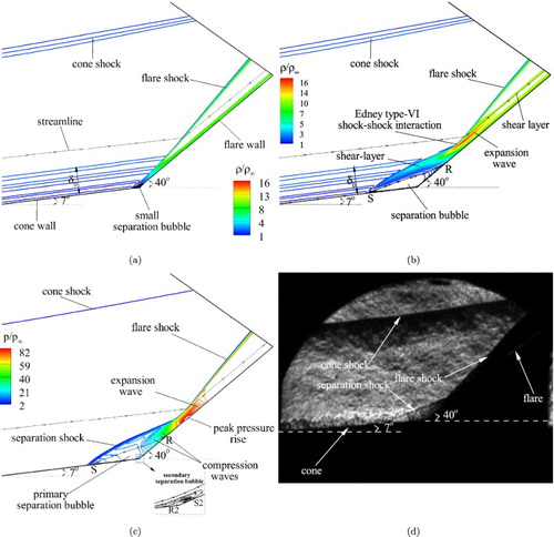
The computed results using the shock-unsteadiness modified SA turbulence model are shown in Figures 3(b) and 3(c). A shock-unsteadiness parameter of is used in the numerical simulation. The separation bubble at the corner generates a separation shock and reattachment shock waves. These reattachment shock waves coalesce to form a flare shock. The separation and flare shock interact to form a shock–shock type-VI interaction (Edney, 1968). This shock–shock interaction is not as prominently predicted by the SA model (see Figure 3(a)). At the shock–shock intersection, an expansion wave and high entropy shear layer emanate. The expansion fan interacts with the compressed boundary layer on the flare surface and is reflected as shown in Figure 3(c). The modified SA model yields a larger separation as compared to the standard SA model and hence the shock pattern is found to match qualitatively the experimental image shown in Figure 3(d). Although the shock structure observed in the Schlieren image is vague, its influence on the wall pressure is however measurable and is shown in Figure 4(a).

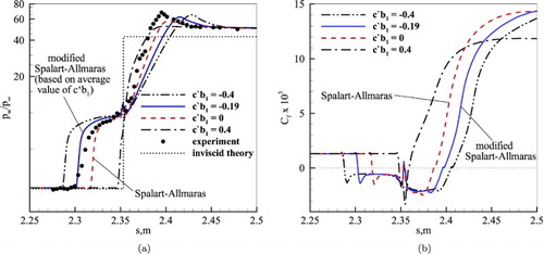
Figure 4. Case-1: computed wall pressure (a) and skin-friction coefficient (b) using the standard SA model (Spalart & Allmaras, 1992) and the shock-unsteadiness modified SA model (Sinha et al., 2005), compared to the experiments of Holden et al. (2014) at Mach 8.

The variation of normalized wall pressure and skin friction, , is shown in Figure 4. There is no available experimental data on for these cases to compare with the presented computed results. The standard SA model in Figure 4(a) predicts a delayed initial pressure rise at as compared to experiment. Due to the adverse pressure gradient across the separation shock, the flow separates. Hence the velocity gradient is zero, resulting in skin-friction coefficient at the separation point S. At the reattachment point R, again . In the separation zone, takes negative values because of flow reversal. The separation bubble size is evaluated as the distance between S and R along the wall stream-wise direction, s. In the reattachment region, as the boundary layer is compressed, a higher velocity gradient results and therefore a higher . A small separation bubble size of is predicted by the SA model as shown in Figure 4(b). Also, this turbulence model does not match the peak pressure rise at the reattachment region R in Figure 4(a). The decline in pressure after R is not as noticeable, since it does not generate an expansion wave at the shock–shock interaction. This shows that an inaccurate prediction of the initial pressure rise location by the SA model results in an erroneous separation bubble size and hence results in an incorrect shock structure as compared to experiment.

The modified SA model shows an initial pressure rise location at , mimicking experiment. Also, the plateau in the separation bubble is predicted relatively more accurately; however, it misses the shock location at R. The small rise in pressure at the corner () is due to secondary flow separation and is shown in the inset of Figure 3(c). The peak rise of pressure at the reattachment region, R, is also close to that found in experiment as compared to the standard SA model. The wall pressure drops across expansion waves at after the reattachment region R (see Figure 3(c)) and matches experiment far downstream. The modified SA model predicts a separation bubble length of as shown in Figure 4(b). Both models match the inviscid pressure rise across the cone shock (Anderson, 2004). A higher pressure is predicted as compared to inviscid theory after the flare shock by both models. This is caused by an additional pressure rise due to multiple compression waves and the effect of the influence of higher pressure generated at the shock–shock interaction on the wall as shown in Figure 3(c). The experimental data upstream of is itself not exactly uniform and is most likely due to free-stream disturbances present in the flow. Only a couple of points lie within the computational data. Thus, there is a slight disagreement in the range .

The skin-friction data show a large negative region between the S and R points, most likely from reversing flow in the separation region, and show positive values at the corner in the secondary flow region. The boundary layer is compressed across the flare shock as shown in Figure 3(a) by the SA model, which therefore results in higher velocity gradients in the near-wall region. Hence, it predicts higher values of downstream of the reattachment region R. The modified SA model shows higher values downstream of R as compared to the standard SA model because of additional compression of the boundary layer across compression shocks and the flare shock (see Figures 3(c) and 3(d)).

Figure 2(b) shows that the model parameter takes positive values for lower values of less than 2.1 and takes negative values for greater than 2.1. Figure 2(a) shows that takes low values near the wall and takes higher values away from wall. Therefore, locally, takes positive values near the wall and negative values away from the wall (see Figure 2(b)). Therefore, the limitation of the shock-unsteadiness Spalart–Allmaras model is that is calculated based on the average value of rather than the local values as plotted in Figure 2(a). The detailed calculation of is discussed in an article by Pasha and Sinha (2012) and is not presented in the current work. The parametric analysis of is discussed for case-2 in Figures 6(a) and 6(b). It is observed that the value of is very sensitive in the determination of the initial separation point location: results in a larger separation bubble and results in incipient separation. When in Equation (4(4) ), the source term becomes , no correction is applied, and both the SA and modified SA models match to give the same result. In the current simulation, an average value of is evaluated from an average value of and is used for case-2 simulation. The computed density contours using the modified SA model are compared to the experimental Schlieren image for case-2 at Mach 7 (see Table 1) in Figure 5. The separation shock length closely matches qualitatively that found in experiment. The shock–shock interaction region does not appear to be as clear in the experimental Schlieren image in Figure 5(b). A thick boundary layer in Figure 5(a) is compressed across the separation shock and bifurcates into two parts. Part of it forms a separated region and part of it flows above the separation bubble and becomes further compressed across the reattachment shock.

Figure 5. Case-2: computed normalized density contours using the shock-unsteadiness modified SA model (Sinha et al., 2005) (a) compared to the Schlieren image of Holden et al. (2014) at Mach 7 (b).

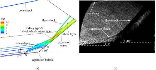
Figure 6. Case-2: computed wall pressure (a) and skin-friction coefficient (b) using the standard SA model (Spalart & Allmaras, 1992) and the shock-unsteadiness modified SA model (Sinha et al., 2005), compared to the experiments of Holden et al. (2014) at Mach 7.

The SA model predicts the delayed initial pressure rise location in Figure 6(a) and thereby results in a small separation bubble size of (see Figure 6(b)). The initial pressure location is predicted accurately by modified SA model in Figure 6(a) and thereby results in a separation bubble size of in Figure 6(b). The predicted peak pressure rise is also close to experiment as compared to the SA model. The computed R location is shifted downstream by both models as compared to experiment, as shown in Figure 6(a). A lower value of inviscid pressure rise to oblique shock at the flare-corner for the current case ( = 7) than the former case ( = 8) would lead to a lower separation bubble. But an opposite trend is observed – the separation bubble, in this case, is more than the earlier case with = 8. The reasons for this trend are explained as follows. The separation bubble size in shock/boundary-layer interaction compression corner flows depends on the free-stream Mach number, the Reynolds number, the wall temperature, and the deflection angle (Elfstrom, 1972). It is observed that a boundary layer that has more turbulent kinetic energy is likely to delay separation and reattach faster than with a lower value (Pasha, 2018). Therefore, the flow at a higher Mach number is likely to have a smaller separation bubble in case-1 than in case-2. Secondly, case-2 is found to have a relatively hotter wall () than case-1 (). A hotter wall with higher values of decreases the local Reynolds number and hence increases the separation bubble size. Also, a higher Reynolds number in case-2 (see Table 1) would result in a lower boundary-layer thickness upstream of the interaction as compared to case-1 (see Figures 3(a) and 5(a)). Overall, case-2 results in a larger shock/boundary-layer interaction region at the flare corner than case-1.

The computed flowfield using the modified SA model is depicted by the density contours in Figure 7(a) for case-3 and is compared to the experiment image in Figure 7(b). Expansion waves are generated (see Figure 7(a)) on the upper surface of the separation bubble. These expansion waves extend and form a train of waves between the shear layer generated in the shock–shock interaction region and boundary layer on the flare wall. Secondly, the expansion fan generated at the shock–shock interaction overlaps with this expansion fan train and forms a complex region. This complex expansion wave region is also observed in case-4 and is depicted by density contours in Figure 8(a). In both case-3 and case-4, the modified SA model qualitatively predicts a separation shock length close to that of the experimental Schlieren images in Figures 7(b) and 8(b) at the corner. Again, the shock–shock interaction region flowfield features are vague in these Schlieren images.

Figure 7. Case-3: computed normalized density contours using the shock-unsteadiness modified SA model (Sinha et al., 2005) (a) compared to the experimental Schlieren image of Holden et al. (2014) at Mach 6 (b).

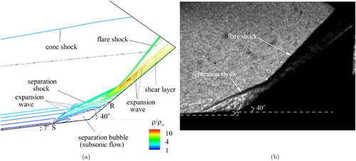
Figure 8. Case-3: computed wall pressure (a) and skin-friction coefficient (b) using the standard SA model (Spalart & Allmaras, 1992) and the shock-unsteadiness modified SA model (Sinha et al., 2005), compared to the experiments of Holden et al. (2014) at Mach 6.

The computed results for case-3 and case-4 using the SA model results in a large separation bubble as shown by the wall pressure and variations in Figures 9 and 10. This is because of lower predicted values of the eddy viscosity by the SA model for these cases. The SA model predicts an early initial pressure rise location as compared to experiment, as shown in Figures 9(a) and 10(a), and hence results in larger separation bubble size as shown by the plots in Figures 9(b) and 10(b). Similar variation is observed in shock/boundary-layer interaction flows at low Mach numbers (Sinha et al., 2005). The shock-unsteadiness model applies a correction to the SA model by modifying the eddy viscosity by accounting for the unsteady effects resulting from the shock–turbulence interaction. This is achieved by implementing the positive values of model parameter for case-3 and for case-4 in the source term . The positive values of for these cases is due to the lower average values of obtained in the simulation (see Figure 2(b)). As the correction is applied only across the shock wave and is negative across it, a positive value of and a negative value of results in a positive value of source term for low Mach flows. This is contrary to case-1 and case-2, where negative values of were used resulting in negative values of the source term for high Mach flows. The positive values of result in higher values of eddy viscosity production and hence results in delayed separation. Therefore, the modified SA model closely matches the initial pressure rise location found by experiment as shown in Figures 9(a) and 10(a). It is to be noted that the initial pressure rise location predicted by the modified SA model is close to that predicted by the SA model. This is due to the values being close to zero (see Figure 2(b)). However, this problem is aggravated for low Mach flows where the SA model results in very large separation bubble size (Sinha et al., 2005). The variation in wall pressure on the cone surface up to the corner is predicted accurately by the modified model as compared to the SA model. An offset in pressure rise after the corner is observed by both models as compared to experiment. An accurate initial pressure location results in an accurate separation point location S as depicted by in Figures 9(b) and 10(b). This leads to an accurate prediction of separation bubble size as compared to the SA model. It is observed that all four cases predict the initial pressure rise location at (see Figures 4(a), 6(a), 9(a) and 10(a)), regardless of different upstream Mach number, Reynolds number, and wall temperature conditions.

Figure 9. Case-4: computed normalized density contours using the shock-unsteadiness modified SA model (Sinha et al., 2005) (a) compared to the Schlieren image of Holden et al. (2014) at Mach 5 (b).

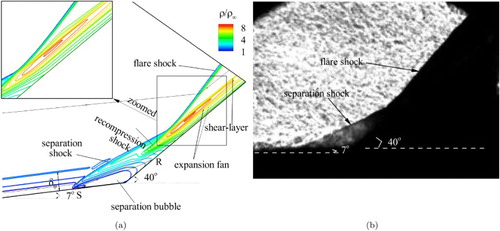
Figure 10. Case-4: computed wall pressure (a) and skin-friction coefficient (b) using the standard SA model (Spalart & Allmaras, 1992) and the shock-unsteadiness modified SA model (Sinha et al., 2005), compared to the experiments of Holden et al. (2014) at Mach 5.

Figure 4(a) shows that the gradual pressure rise across weak compression waves (see Figure 3(c)) associated with the boundary layer separation is not very well predicted by the shock-unsteadiness modified SA model in the shock/boundary-layer interaction region between s=2.35 and . Similar behavior is observed in the current case-4 (see Figure 10(a)) and the former case-2 and case-3 (see Figures 6(a) and 9(a)) by both the standard and the modified SA models. This is because the shock-unsteadiness correction was developed by Sinha et al. (2003) for homogeneous isotropic turbulence interaction with a strong compression wave (normal shock wave). Hence, it may have limitations in flows with weak compression waves (Mach waves). However, the shock-unsteadiness model has been found to perform well in shock/boundary-layer interaction flows with incipient separation, for example a 6–36 cone–flare at Mach 11 (Pasha & Sinha, 2012).

The computed heat-transfer rate, , is based on Fourier's law of heat conduction in the near-wall region and is calculated as . Here, is the wall temperature, is the normal distance at the first cell center from the wall, is the temperature at , and . The thermal conductivity is assumed to be a function of average temperature T and is modeled as a 6th-order polynomial curve with an accuracy of , which is justified (Holman, 2009). The heat-flux rate variation in the shock/boundary-layer interaction region is shown in Figure 11(a). The plateau is not predicted accurately by either of the two models in the interaction region. The SA model predicts close to the measured values near the corner region, whereas the modified SA model deviates. Both turbulence models under-predict the heat-transfer rate at the reattachment region with the modified SA model close to experiment. The presence of a noticeable fluctuation in the heat-transfer trace in the later part of the junction region is indicative of highly energetic reversing flow. Slight fluctuations in the heating trace at the start of the junction region confirm the presence of a secondary system squeezed ahead of the main vortex system in the junction region. Both models tend to under-predict the peak heating loads at Mach 5 for case-4 (Figure 11(b)).

Figure 11. Computed heat-transfer rate for (a) case-1 at Mach 8 and (b) case-4 at Mach 5, compared to the experiments of Holden et al. (2014).

Zhang et al. (2017) improved the heat flux in the shock/turbulent boundary-layer interaction flow in an axisymmetric cone–cylinder–flare body at Mach 7. In their work, a shock wave detector based on non-dimensional pressure is developed based on the smooth measurement factor method proposed in the construction of the WENO scheme (higher-order scheme) by Jiang and Shu (1996). Also, the shear stress transport (SST) k–ω turbulence model is modified to dampen the production of turbulent kinetic energy near the shock wave. The distribution of heat flux shows that the modified SST k–ω model (Menter, 1994) has no influence on the flow separation as compared to its original predictions. The modified model, however, does reduce the heat flux in the reattachment region when compared against results from the original model. Overall, it can be concluded that the heat flux distribution in the separation bubble is predicted closer to experiment, which is attributed to using the higher-order WENO scheme. In the current work, the physical implementation of the modified SA model improves the prediction of the separation bubble in the shock boundary-layer interaction region when compared to the original SA model. The numerical scheme (WENO) as implemented by Zhang et al. (2017) can further improve the heat flux distribution in the separation region from 2.3 to as observed in Figure 11. Also, the scheme is better able to resolve the pressure distribution in the plateau region of the separation bubble (s=2.3 to ) as well as in the downstream regions from s=2.35 to (see Figures 4(a),  6(a), 9(a), and 10(a)).

In a recent work, the turbulent-energy heat flux for isotropic homogeneous shock–turbulence interaction was modeled in terms of varying Prandtl number and the results matched the DNS data accurately (Quadros & Sinha, 2016; Quadros, Sinha & Larsson, 2016). This model when implemented on oblique shock/boundary-layer interaction flows at Mach 5 improved the heat-transfer predictions in the reattachment region (Roy, Pathak, & Sinha, 2018). Future work will be directed towards computing the heat-transfer rate to the current cone–flare configuration by implementing this model.

4. Conclusions

Reynolds-averaged Navier–Stokes based computations were carried out to investigate the shock/boundary-layer interaction on a cone–flare geometry in a hypersonic flow. The computations confirm the presence of a separated flow region at the junction region. The boundary layer developing past the separation region and the shock emanating from the reattachment location supports a complex shock region with expansion waves emanating from the shock and the high entropy region. The physics-based source term in the standard Spalart–Allmaras turbulence model accounts for the unsteady effects and leads to an improvement in all cases to the prediction of the initial pressure rise location and the separation bubble size, and hence also the shock structure. The model parameter has limitations in that it depends on an average value of the Mach number normal to the shock wave instead of the local value, and further research work is required in this direction. The shock-unsteadiness model fails to predict the heat-transfer flux both in the separation region and downstream of it. Further improvements to the present shock-unsteadiness model are envisaged by accounting for the turbulent-energy heat flux in cone–flare configuration studies.

Acknowledgments

The authors would like to thank the Dean of Engineering, King Abdulaziz University, Jeddah, for providing the necessary facilities to carry out the research. The simulations in this work were performed at the High Performance Computing Center (Aziz Supercomputer) (http://hpc.kau.edu.sa). The authors would also like to thank Professor Krishnendu Sinha from the Department of Aerospace Engineering, Indian Institute of Technology Bombay, Mumbai, India for his kind help, and all the reviewers for their valuable suggestions.

Disclosure statement

No potential conflict of interest was reported by the authors.

ORCID

Amjad Ali Pasha http://orcid.org/0000-0003-1750-4574

K. A. Juhany http://orcid.org/0000-0002-5612-0605

M. Khalid http://orcid.org/0000-0003-4389-0691

Additional information

Funding

This article was funded by the Deanship of Scientific Research (DSR) at King Abdulaziz University, Jeddah. The authors, therefore, acknowledge with thanks DSR for technical and financial support.

References

- Anderson, J. D., Jr (2004). Modern compressible flow with historical perspective (3rd ed.) (pp. 366–371). New York: McGraw-Hill.
- Bose, D., Brown, J. L., Prabhu, D. K., Gnoffo, P., Johnston, C. O., & Hollis, B. (2013). Uncertainty assessment of hypersonic aerothermodynamics prediction capability. Journal of Spacecraft and Rockets, 50(1), 12–18. DOI:doi: 10.2514/1.A32268
- Brown, J. L. (2013). Hypersonic shock wave impingement on turbulent boundary layers: Computational analysis and uncertainty. Journal of Spacecraft and Rockets, 50(1), 96–123. DOI:doi: 10.2514/1.A32259
- Catris, S., & Aupoix, B. (2000). Density corrections for turbulence models. Aerospace Science and Technology, 4(1), 1–11. DOI:doi: 10.1016/S1270-9638(00)00112-7
- DeBonis, J. R., Oberkampf, W. L., Wolf, R. T., Orkwis, P. D., Turner, M. G., Babinsky, H., & Benek, J. A. (2012). Assessment of computational fluid dynamics and experimental data for shock boundary-layer interactions. AIAA Journal, 50(4), 891–903. DOI:doi: 10.2514/1.J051341
- Deck, S., Duveau, P., d’Espiney, P., & Guillen, P. (2002). Development and application of Spalart–Allmaras one-equation turbulence model to three-dimensional supersonic complex configurations. Aerospace Science and Technology, 6(3), 171–183. doi: 10.1016/S1270-9638(02)01148-3
- Druguet, M. C., Candler, G. V., & Nompelis, I. (2005). Effects of numerics on Navier–Stokes computations of hypersonic double-cone flows. AIAA Journal, 43(3), 616–623. doi: 10.2514/1.6190
- Edney, B. E. (1968). Anomalous heat-transfer and pressure distributions on blunt bodies at hypersonic speeds in the presence of an impinging shock (Report No. FFA–115). Stockholm: The Aeronautical Research Institute of Sweden.
- Elfstrom, G. M. (1972). Turbulent hypersonic flow at a wedge-compression corner. Journal of Fluid Mechanics, 53(1), 113–127. doi: 10.1017/S0022112072000060
- Gaitonde, D. V. (2015). Progress in shock-wave/boundary-layer interactions. Progress in Aerospace Sciences, 72, 80–99. DOI:doi: 10.1016/j.paerosci.2014.09.002
- Guohua, T. U., & Xiaogang, D. (2012). Assessment of two-equation turbulence models and some compressibility corrections for hypersonic compression corners by high-order difference schemes. Chinese Journal of Aeronautics, 25(1), 25–32. doi: 10.1016/S1000-9361(11)60358-0
- Holden, M. S. (1991). Studies of the mean and unsteady structure of turbulent boundary-layer separation in hypersonic flow. In 22nd Fluid Dynamics, Plasma Dynamics and Lasers Conference, Honolulu, HI, Paper No. AIAA-1991-1778.
- Holden, M. S., Wadhams, T. P., & MacLean, M. (2014). Measurements in regions of shock wave/turbulent boundary-layer interaction from Mach 4 to 10 at flight duplicated velocities to evaluate and improve the models of turbulence in CFD codes. DTIC Document. CUBRC, Inc.
- Holman, J. P. (2009). Heat transfer (10th ed.). Boston, MA: McGraw-Hill Higher Education.
- Jiang, G. S., & Shu, C. W. (1996). Efficient implementation of weighted ENO schemes. Journal of Computational Physics, 126(1), 202–228. doi: 10.1006/jcph.1996.0130
- Knight, D. D., & Degrez, G. (1998). Shock wave turbulent boundary layer interactions in high Mach number flows – a critical survey of current numerical prediction capabilities (Technical Report AGARD-AR-319-02). Neuilly sur Seine, France: Advisory Group for Aerospace Research and Development, NATO.
- Knight, D., Yan, H., Panaras, A. G., & Zheltovodov, A. (2003). Advances in CFD prediction of shock wave turbulent boundary layer interactions. Progress in Aerospace Sciences, 39(2–3), 121–184. doi: 10.1016/S0376-0421(02)00069-6
- MacCormack, R. W., & Candler, G. V. (1989). The solution of Navier–Stokes equations using Gauss–Siedal line relaxation. Computers and Fluids, 17(1), 135–150. doi: 10.1016/0045-7930(89)90012-1
- Marvin, J. G., Brown, J. L., & Gnoffo, P. A. (2013). Experimental database with baseline CFD solutions: 2-D and axisymmetric hypersonic shock-wave/turbulent boundary-layer interactions (NASA TM-2013-216604). Moffett Field, CA: NASA Ames ResearchCenter.
- Menter, F. R. (1994). Two-equation eddy-viscosity turbulence models for engineering applications. AIAA Journal, 32(8), 1598–1605. DOI:doi: 10.2514/3.12149
- Nompelis, I. (2004). Computational study of hypersonic double-cone experiments for code validation (Doctoral dissertation). University of Minnesota, Minneapolis and Saint Paul, MN, pp.119–225.
- Panaras, A. G. (2015). Turbulence modeling of flows with extensive crossflow separation. Aerospace, 2, 461–481. doi: 10.3390/aerospace2030461
- Pasha, A. A. (2012). Application of shock-unsteadiness modification to hypersonic shock/turbulent boundary-layer interaction (Doctoral dissertation). Indian Institute of Technology Bombay, Mumbai, India, pp.44–45.
- Pasha, A. A. (2018). Study of parameters affecting separation bubble size in high speed flows using k–? turbulence model. Journal of Applied and Computational Mechanics, 4(2), 95–104. doi: 10.22055/jacm.2017.22761.1140
- Pasha, A. A., & Sinha, K. (2008). Shock-unsteadiness model applied to oblique shock-wave/turbulent boundary-layer interaction. International Journal of Computational Fluid Dynamics, 22(8), 569–582. doi: 10.1080/10618560802290284
- Pasha, A. A., & Sinha, K. (2012). Shock-unsteadiness model applied to hypersonic shock wave/turbulent boundary-layer interactions. Journal of Propulsion and Power, 28(1), 46–60. DOI:doi: 10.2514/1.B34191
- Quadros, R., & Sinha, K. (2016). Modelling of turbulent energy flux in canonical shock–turbulence interaction. International Journal of Heat and Fluid Flow, 61, 626–635. DOI:doi: 10.1016/j.ijheatfluidflow.2016.07.006
- Quadros, R., Sinha, K., & Larsson, J. (2016). Turbulent energy flux generated by shock/homogeneous turbulence interaction. Journal of Fluid Mechanics, 976, 113–157. DOI:doi: 10.1017/jfm.2016.236
- Roy, C. J., & Blottner, F. G. (2006). Review and assessment of turbulence models for hypersonic flows. Progress in Aerospace Sciences, 42(7–8), 469–530. doi: 10.1016/j.paerosci.2006.12.002
- Roy, S., Pathak, U., & Sinha, K. (2018). Variable turbulent Prandtl number model for shock/boundary-layer interaction. AIAA Journal, 56(1), 342–355. doi: 10.2514/1.J056183
- Sanders, R., Morano, E., & Druguet, M. C. (1998) Multidimensional dissipation for upwind schemes: stability and applications to gas dynamics. Journal of Computational Physics, 145(2), 511–537. doi: 10.1006/jcph.1998.6047
- Sinha, K., & Candler G. V. (1998). Convergence improvement of two-equation turbulence model calculations. In 29th AIAA Fluid Dynamics Conference, Albuquerque, NM, Paper No. AIAA-Paper-1998-2649.
- Sinha, K., Mahesh, K., & Candler, G. V. (2005). Modeling the effect of shock-unsteadiness in shock/turbulent boundary-layer interactions. AIAA Journal, 43(3), 586–594. DOI:doi: 10.2514/1.8611
- Sinha, K., Mahesh, K., & Candler, G. V. (2003). Modeling shock-unsteadiness in shock/turbulence interaction. Physics of Fluids, 15(8), 2290–2297. DOI:doi: 10.1063/1.1588306
- Spalart, P. R., & Allmaras, S. R. (1992). A one-equation turbulence model for aerodynamic flows. In 30th Aerospace sciences meeting and exhibit, Reno, NV, Paper No. AIAA-1992-0439.
- Wilcox, D. C. (2000). Turbulence modeling for CFD (2nd ed.). La Cañada, CA: DCW Industries.
- Wright, M. J., Candler, G. V., & Bose, D. (1998). Data-parallel line relaxation method for the Navier–Stokes equations. AIAA Journal, 36(9), 1603–1609. doi: 10.2514/2.586
- Wright, M. J., Sinha, K., Olejniczak, J., Candler, G. V., Magruder, T. D., & Smits, A. J. (2000). Numerical and experimental investigation of double-cone shock interactions. AIAA Journal, 38(12), 2268–2276. doi: 10.2514/2.918
- Yang, Z. (2015). Large-Eddy simulation: Past, present and the future. Chinese Journal of Aeronautics, 28(1), 11–24. doi: 10.1016/j.cja.2014.12.007
- Zhang, Z., Gao, Z., Jiang, C., & Lee, C. H. (2017). A RANS model correction on unphysical over-prediction of turbulent quantities acrossshock wave. International Journal of Heat and Mass Transfer, 106, 1107–1119. doi: 10.1016/j.ijheatmasstransfer.2016.10.087