Three-dimensional simulation of a self-propelled fish-like body swimming in a channel

ABSTRACT

In this study, a three-dimensional simulation of a fish-like body swimming in a channel with non-slip walls was carried out to investigate the effects of kinematics on swimming performance. Self-propelled swimming in an inertial coordinate system was examined by using the direct forcing immersed boundary method. The fish body consisted of several rigid bodies and behaved analogously to a multi-segment robotic fish. The computational program was first validated by simulating fluid flow around a circular cylinder at Reynolds number (Re) =100 and Re = 1000, as well as around a settling particle. The results were compared with experimental and numerical results from past research in the area. A virtual parametric study of the tail-beat frequency, phase difference between neighboring body segments, and body amplitude was then conducted. The effect of the lateral and vertical distance between the model body and walls on swimming performance is also discussed. The results for the velocity and vorticity fields around the model body provided evidence for the mechanism of thrust generation and highlighted the effects of kinematics on swimming performance.

KEYWORDS:

• Fish-like swimming
• immersed boundary method
• self-propelled
• tail-beat frequency
• phase difference
• amplitude

Introduction

Fish are sophisticated swimmers that exhibit interesting hydrodynamic features. It has been shown that separation elimination, turbulence reduction, and energy extraction from oncoming flow are used in fish-like locomotion (Triantafyllou et al., 2002). Flow phenomena concerning swimming fish have attracted research interest from a variety of fields. Such studies can yield a better understanding of the flow control mechanism for efficient propulsion and high stability, and inspire such engineering applications as bionic underwater machines (Liu & Hu, 2010).

The swimming mode adopted by a single type of fish is a compromise between propulsion efficiency and other aspects, such as predator avoidance (Sfakiotakis, Lane, & Davies, 1999). Moreover, factors like turbulence may also affect swimming behavior (Liao, 2007), while the kinematics of the models of burst and efficient swimming can be different (Kern & Koumoutsakos, 2006). The swimming modes of fish can be generally divided into body/caudal fin (BCF) undulation and median/paired fin (MPF) movement (Sfakiotakis et al., 1999). Most fish use BCF for propulsion whereas MPF is frequently used for stability and maneuverability (Borazjani & Sotiropoulos, 2008). To study these modes of swimming in fish, theoretical analysis (Wu, 2001), numerical simulations of deforming surfaces, imitation by robotic fish, and experiments employing real organisms are considered effective approaches to gaining a comprehensive understanding of aquatic locomotion (Lauder & Drucker, 2002). As a fundamental approach to studying the swimming phenomena, numerous experiments have been carried out, and have provided valuable data to help understand the kinematics and hydrodynamics of fish locomotion. Many such experiments employed live fish (Webber, Boutilier, Kerr, & Smale, 2001), while dead fish were used in some cases (Beal, Hover, Triantafyllou, Liao, & Lauder, 2006; Long, Mchenry, & Boetticher, 1994). In addition to using real fish, artificial underwater mechanisms such as oscillating foils (Anderson, Streitlien, Barrett, & Triantafyllou, 1998) and fish-like robots (Barrett, Triantafyllou, Yue, Grosenbaugh, & Wolfgang, 1999; Epps, Alvarado, Youcef-Toumi, & Techet, 2009) have also frequently been adopted.

With the development of computational technology, numerical simulations are becoming ever more important to investigate various flow phenomena. Many case studies have applied computational fluid dynamics (CFD) to these problems (Narasimha, Brennan, & Holtham, 2007; Stamou, Katsiris, Politis, & Schaelin, 2008; Wang, Reitz, Pera, Wang, & Wang, 2013). For studies of swimming fish, numerical studies have also provided insightful results, some of which may be difficult to obtain experimentally. For example, three-dimensional (3D) flow fields and vorticity structures can be directly visualized and studied by performing 3D simulations (Liu & Kawachi, 1999; Zhu, Wolfgang, Yue, & Triantafyllou, 2002), and parametric studies, such as those for Reynolds number (Re) and Strouhal number (St), can be carried out by controlling the computational conditions (Borazjani & Sotiropoulos, 2008).

To address issues related to swimming fish, many numerical studies have used experimental data based on live fish as inputs to the kinematics used for simulations. However, there are far fewer results drawn from virtual swimming studies, such as those generated by changing the combination of parameters related to swimming kinematics beyond the ranges employed by fish in experimental observations. This virtual swimming allows exploration of flow phenomena that are challenging to implement in experiments using real fish. One example is the study on the effects of body shape and kinematics on the hydrodynamics of BCF swimming by Borazjani and Sotiropoulos (2010). They conducted simulations of self-propelled virtual swimmers, such as those with anguilliform kinematics but carangiform body shapes. However, 3D simulations of self-propelled models have rarely been examined. Instead, studies typically include limitations on movement axes; for example, movement was restricted in the streamwise direction in the study by Borazjani and Sotiropoulos (2010).

Therefore, the goal of this study is to conduct a 3D simulation of self-propelled swimming in which not only the model itself, but also the range of its movement is in three dimensions. A parametric analysis of tail-beat frequency, phase difference, and tail-beat amplitude is performed in the context of virtual swimming. In contrast to the work in Borazjani and Sotiropoulos (2010), where the governing equations are formulated in a non-inertial frame of reference to simulate self-propelled swimming, the governing equations in this study are formulated in an inertial coordinate system. The shape and kinematics of a fish-like model, formulated in several body-fixed frames of references, are transformed into the inertial frame of reference. The simulation of a fish-like body in flow requires considering fluid–structure interactions (FSIs), for which the immersed boundary method has been frequently adopted (Borazjani, Ge, & Sotiropoulos, 2008; Fauci & Peskin, 1988; Luo, Wang, & Fan, 2007). In this study, the direct forcing approach is used to generate a model of fish-like swimming motion. The movement of the fish body is defined in relation to other structures, rather than by designating one function to represent the entire body, as has usually been the norm in the literature. This modeling method is considered more representative of real fish, and is more applicable to artificial machines, such as robotic fishes. A feedback mechanism is used to implement the beginning of the swimming process, driven by a hydrodynamic force generated by the undulatory movement of the model. In addition to validating the feasibility and effectiveness of this approach, 3D swimming performance and the flow field in virtual modes are investigated. More informative and accurate results concerning the hydrodynamics of fish swimming are expected. The following section provides illustrations and descriptions of the proposed computational model and the relevant conditions. A validation of this program is subsequently provided, including the flow around a circular cylinder and a single settling particle in fluid. The results are then presented and discussed, and the conclusions of this study are drawn.

Computational model and conditions

Nomenclature

P	=	Pressure
	=	Velocity
	=	Velocity of the origin point of the body-fixed coordinate system(s)
	=	Reynolds number
	=	Time
	=	Body force
	=	Surface force
	=	Fluid field
	=	Field inside the immersed boundary
	=	Velocity inside the immersed boundary
	=	Desired velocity inside the immersed boundary
	=	Location vector in the inertia coordinate system
	=	Location vector of the origin point of the body-fixed coordinate system (1) in the inertial coordinate system
	=	Location vector in the body-fixed coordinate system (1)
, ,	=	Unit vectors of the inertia coordinate system
, ,	=	Unit vectors of the body-fixed
(s = 1,2, … ,7)	=	coordinate system(s)
, ,	=	Coordinates of the origin point of the body-fixed coordinate system (1) in the inertial coordinate system
x, y, z	=	Coordinates in the inertial coordinate system
, ,	=	Coordinates in the body-fixed coordinate system (1)
	=	External force
	=	Fluid density
	=	Setting mass of the model
	=	Acceleration of the model
	=	Acceleration of fluid
	=	External torque
	=	Inertia matrix
, a, b, c	=	Constants
	=	Wall normal unit vector
	=	Vector from the origin of to the point to be identified
	=	Angular velocity of the model
	=	Angular velocity of the body-fixed coordinate system(s)
	=	Angular acceleration of the model
	=	Location vector of the center of mass of the model in the inertia coordinate system
, ,	=	Size parameters of the model
	=	Undulatory amplitude
	=	Undulatory angular velocity
	=	Phase difference between the neighboring parts of the model

The non-dimensional Navier–Stokes equations for incompressible fluid containing a body force can be expressed as: (1) (2) (3)

Note that in Equation (3), the flow velocity is defined at all grid nodes inside the immersed boundary rather than those merely in the vicinity of the boundary. A direct forcing approach following a principle introduced by Balaras (2004) is employed to calculate the body force, which is updated at each time step to obtain the desired velocity within the boundary. According to Hirose, Kihara, and Abe (2012), the concept can be explained as follows.

The discrete form of Equation (1) is (4) where denotes . Inside the immersed boundary, velocity is defined as , the desired velocity at the time step n+1: (5)

The body force can be obtained as (6) No body force is imposed on the fluid outside the immersed boundary. The calculation of the body force can be summarized as (7)

In this study, to satisfy the continuity condition of Equation (2), the fish model is designed as a rigid-body system analogous to the robotic mechanism employed in the literature (Barrett et al., 1999). Figure 1 shows the schematic geometrical configuration and size of the simplified model, which consists of an ellipsoid head with semi-principal axes with lengths of , and a body part composed of four blocks and a triangular tail. The undulatory movement of the body is implemented by controlling the relative rotation around the vertical axes (3, 4, 5, 6) as shown in Figure 1. Dorsal or pectoral fins are not considered for the sake of simplicity.

Figure 1. Computational model and dimensions ().

Figure 2 shows the body-fixed coordinate systems used to define the boundaries of the immersed body and the relative rotation of each part. The number of rotational axes corresponds to those in Figure 1 (Axis number 7 is attached to the end of the tail). The x–z planes of all body-fixed coordinate systems are confined to one plane. Thus, all y-axes are parallel. The distances between pairs of neighboring origins (for example ) are fixed. This setting allows for a transverse undulation of the model to imitate fish-like swimming. As indicated in Figure 2, the first coordinate system for the ellipsoid head coincides with the second one, and the last coordinate system, numbered 7, has unit vector along the same direction as the preceding one, numbered 6, but with a different origin.

Figure 2. Body-fixed coordinate systems.

The formula for the inside–outside judgement for the ellipsoid, block, and cylindrical surfaces used in constructing the model are derived in the body-fixed coordinate systems, and are listed in Table 1. In the case of the ellipsoid, for example, the location of an inside point P is denoted by in the inertial coordinate system, which is equal to , where the subscripts x, y, and z refer to the components of the inertial system. is the coordinate in the body-fixed system calculated from the coordinates in and through the matrix in Table 1, which is then used to perform inside–outside judgement in the equation for the ellipsoid. For the block and cylindrical surfaces, a unit vector is set for position.

Table 1. Formula for inside–outside judgement.

	Schematic diagram	Formula
Ellipsoid		where The subscripts x, y, z denote the components in the inertial system.
Block plane		where is the wall normal unit vector, is the vector from the origin of to the point to be identified.
Cylindrical surface		where is the unit vector, with direction along the central axis of the cylinder, is the vector from the origin of to the point to be identified.

The center of mass is assumed to always be at the center of the ellipsoid for the sake of simplicity; the movement of the model is then calculated for this point. Given an initial location and velocity, the kinematics of the corresponding body-fixed system 1 (2) in Figure 2 are computed using Newton's second law of motion for a single rigid body: (8) (9) where and are the external force and the torque acting on the body, respectively. In the above equations, is the setting mass of the fish model, is the acceleration of the center of mass, is angular velocity, and is angular acceleration. In Equation (9), is the inertia matrix that is assumed to take the simple form , where is a constant. Equation (9) can thus be rewritten as (10) For control volume with surface inside, (11) where is the density of the fluid, and and are the body force and the surface force imposed by the surrounding fluid on the control volume, respectively. The integral form of Equation (11) can be written as (12) The second term on the left-hand side of Equation (12) is the total surface force acting on the model. The term on the right-hand side is correlated with the kinematics of the model and reflects the effect of the inertia of the fluid inside the model. The acceleration of each control volume inside may be different, and thus the calculation of this term requires a differential of velocity to obtain the acceleration for each node. This is thought to affect the stability of the simulation as an explicit scheme is used to update the model's velocity, especially when the acceleration is large as in the initial period. Therefore, the right-hand term in Equation (12) is ignored in modeling for the stability of the simulation. Note that the effect of this term on accuracy is thought to become significant only under the condition of relatively high acceleration and low velocity. In this immersed boundary method, the body in flow is modeled by imposing a body force on the fluid inside the immersed boundary. The model can thus be considered part of the fluid in the flow field, and the acceleration and angular acceleration can then be calculated using Equation (12) as (13) (14) where denotes the location vector of the center of mass that is () here. Note that although the right-hand term in Equation (12) is ignored in the modeling, its effect persists, and is considered an additional mass , which is approximately −0.0133. The real density of the fish model is considered similarly to that of the fluid. Thus, to offset the influence of the additional mass on accuracy, especially at the starting stage, the setting mass is chosen to be approximately twice the fluid mass inside the model as . Since rotation is not the main concern in this study, the moment of inertia is set to be relatively large to ensure computational stability, as .

Once the movement of the first (second) body-fixed coordinate system is obtained by the above feedback mechanism, the computational process used to determine the orientations of the body-fixed systems 3 to 6 (denoted by the subscript ‘s’ below), as shown in Figure 2 at time step n + 1, is then set to implement the undulatory movement as (15) (16) where and . The parameter is the relative amplitude of neighboring parts. and are the relative angular velocity and the relative phase difference, respectively, and is time. The initial posture is obtained by letting when . This setting provides a smooth starting process to prevent the abrupt alteration of velocity which may cause unphysical impulse. , , are initially set parallel to the corresponding inertial coordinate axes , , , respectively. From the top view of the model, Figure 3(a) gives a schematic posture to show the relationship between the parameters and the kinematics of the model. To illustrate the effect of on the undulatory mode, the schematic postures of the model using the above definition in a tail-beat cycle with are shown in Figure 3(b). The corresponding velocity and angular velocity are then updated as (17) (18)

Figure 3. (a) Definition of the kinematics (top view); (b) schematic postures in a tail-beat cycle for different phase differences ().

In this study, a 3D channel is defined through a structured grid with domain and grid numbers along the x- (longitudinal), y- (vertical), and z-axes (lateral), respectively, as shown in Figure 4. The outlet boundary condition is specified along the longitudinal direction, and the non-slip wall condition is specified in the lateral and vertical directions. The Reynolds number based on the length of the fish model and the longitudinal velocity ranges from ∼30 to ∼2300 in this study. Note that to improve the efficiency and stability of the simulation, the wall condition is employed. This is not the typical situation for a normal swimming fish and may yield the wall effect on swimming performance. Webb (1993) investigated the swimming performance of steelhead trout in channels with solid or porous walls and highlighted the wall effect on kinematics. However, considering the relatively low Reynolds number in this study, the effect is considered insignificant. A simple assessment of effect of the distance between the pairs of walls along the lateral and vertical directions is shown in the section of results and discussion.

Figure 4. Grid for the simulation.

This study used the open-source CFD code ‘FrontFlow/Red’ (Muto, Tsubokura, & Oshima, 2012; http://www.ciss.iis.u-tokyo.ac.jp/rss21/), which adopts an unstructured finite-volume procedure with vertex-centered-type storage on a grid. The third-order upwind difference scheme is used to discretize the spatial derivatives. The time marching is based on the fractional step method, where the first-order Euler implicit scheme is used to derive the equations for the velocity. The coupling of the velocity and the pressure fields is based on the simplified marker-and-cell (SMAC) method. Due to the use of the third-order upwind spatial scheme and the first-order time marching method, it is necessary to confirm their effects on the computational results. This issue is assessed in the next section, along with a detailed discussion concerning the validation of the computations.

Validation

Flow around a circular cylinder

The proposed computational program, including the direct forcing approach, was first validated by performing simulations of flow around a circular cylinder. The Reynolds number is defined as , where D is the diameter of the cylinder. The simulations were carried out at and 1000, and the results were compared with relevant numerical and experimental results in the literature. For the case where , the computational domain was set to with resolution . For the case where , the flow became 3D and the computational domain was extended in the lateral direction as with resolution . The grid plane perpendicular to the spanwise direction for the two cases is shown in Figure 5, as well as the partial magnification near the cylinder. A resolution of 50 cells was used for the diameter of the cylinder.

Figure 5. Grid plane perpendicular to the spanwise direction: entire view (left) and partial magnification near the cylinder (right).

Figure 6 shows the lift coefficient () and the drag coefficient () against time (where and are the lift and drag forces, respectively, and is the reference area). The time-averaged drag coefficient, the Strouhal number (, where is the oscillation frequency) and the root-mean-square (RMS)-averaged lift coefficient are compared with those from previous studies in Table 2. The results were found to agree well. Figure 7 shows the contours of the instantaneous streamwise velocity on the center planes for the two cases, and the vorticity contours are shown in Figure 8. A Karman vortex street can be seen in the wake flow for , which indicates that the vorticity field was well captured. Figure 9 shows the 3D vortex structures visualized according to the second invariant of the velocity-gradient tensor for the case of , and a similar result can be found in a previous direct numerical simulation (DNS) study (Naito & Fukagata, 2012).

Figure 6. Lift and drag coefficients against time for (left) and 1000 (right).

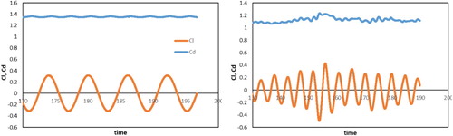
Figure 7. Instantaneous streamwise velocity contours on the center plane for Re = 100 (above) and 1000 (below).

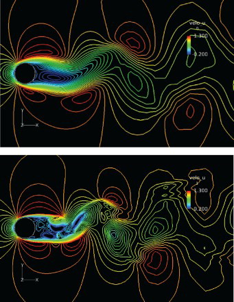
Figure 8. Vorticity contours on the center plane for Re = 100 (above) and 1000 (below). The color scale shows clockwise as blue, and counter-clockwise as red.

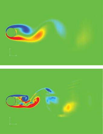
Figure 9. Vortex structures for the case of Re = 1000.

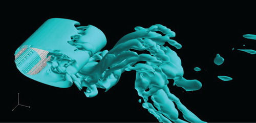
Table 2. Comparison of drag coefficient and Strouhal number with those in previous studies.

	Cd		Cl (RMS)	Cd		Cl (RMS)
Present study	1.35	0.165	0.22	1.13	0.217	0.20
Kim, Kim and Choi (2001)	1.33	0.165	—	—	—	—
Jordan and Fromm (1972)	1.28	0.16	—	1.24	0.206	—
Naito and Fukagata (2012)	1.33	0.165	0.23	1.09	0.21	0.21
Tritton (1959)	1.24–1.26	—	—	—	—	—
Braza, Chassaing, and Minh (1986)	1.30	0.16	—	1.20	0.21	—
Tseng and Ferziger (2003)	1.42	0.164	0.29	—	—	—

Settling particle

The proposed program of the direct forcing approach for moving bodies was validated by simulating the movement of a settling particle in fluid and comparing the obtained velocity with those reported by Mordant and Pinton (2000), and Luo et al. (2007). The density of the fluid was and its kinematic viscosity was . The diameter of the particle was and its density was . The dimension of the computational field was with the resolution and the wall condition for all boundaries. The center of the particle was initially located at (0.002, 0.017, 0.002) with initial velocity . The particle was subject to gravity and reached a limit velocity when the gravity was balanced with drag and buoyancy. The main aim for this validation was to confirm the translation of the particle. Rotation was also included in the simulation, but not considered relevant to the results presented here. Mordant and Pinton (2000) performed an experimental study on a settling particle for different Reynolds numbers and density ratios, and obtained a single exponential relation between vertical velocity and the time to describe the movement as (19) where is particle velocity, is the limit velocity, is time, and is the characteristic time taken for the particle to reach 95% of the limit velocity.

Figure 10 shows the vertical velocity of the particle against time, which agrees well with the profile predicted by Equation (19). A quantitative comparison of limit velocities is provided in Table 3. It is evident that a satisfactory agreement was obtained with previous results in the same conditions.

Figure 10. Velocity profiles for a single settling particle.

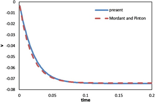
Table 3. Comparison of the limit velocity with past results.

	D (m)	()	(m/s)	Re
Mordant and Pinton (2000)	0.0005	2560	0.0741	41
Luo et al. (2007)			0.0781	44
Present study			0.0745	41

Time step was set to in the settling particle simulation. To assess any dependency on the time-step scale, two cases with larger time steps () were considered and a comparison of the results is shown in Figure 11. As shown, the profiles of settling velocities involving different time steps coincide with one another, indicating that the time-step scale does not significantly influence the simulation results as far as moving boundaries during flow were concerned. In addition to this validation case for the settling particle, the effect of the time-step scale was also assessed for the problem of swimming fish through two test cases (A = 0.25, , ) with time steps of (Baseline) and (Baseline_1). 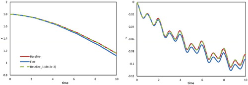Grid dependency was also investigated for the case of swimming fish by performing the same simulation with the baseline case on a finer grid of (Fine). The longitudinal displacement and velocity are shown in Figure 12. By comparing the Baseline and Baseline_1 cases, as in the case of the settling particle, varying the time-step scale had no noticeable effect. For grid dependency, although there was some discrepancy between the Baseline and the Fine cases, it was not significant comparing with those among the cases in the following parametric analysis and the overall features of the swimming process were not considerably affected. Thus, grid dependency was not considered a factor to bring any crucial effect on the final conclusions in this study.

Figure 11. Velocity profiles for a single settling particle with different time steps.

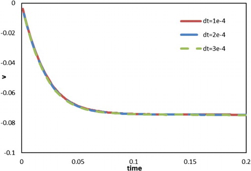
Figure 12. Longitudinal displacement (left) and velocity (right) against time for the cases with different time steps or grids (A = 0.25, , ).

Results and discussion

The effect of the tail-beat frequency on swimming performance was first investigated. Figure 13 shows the displacement (left) and velocity components (right) of the center of mass of the fish-like model against time, for with and A = 0.25. The model started at (1.8, 0.5, 0.5) in the inertia coordinate system, and the time it took to reach the end of the channel decreased approximately linearly with increasing . The indicated linear relationship between swimming velocity and tail-beat frequency has also been reported in past studies (Epps et al., 2009; Long et al., 1994) and can be determined for the lateral component. The forward thrust was the counter-force of that which pushed the fluid backward. With larger , more backward fluid was generated at a higher velocity, resulting in a higher forward thrust and, thus, higher swimming velocity. Conversely, the drag increased with swimming velocity and a limit velocity was achieved when thrust was balanced by drag. This linear relationship between and swimming velocity, and thus longitudinal displacement, indicated a linear relationship between the thrust and , and between drag and swimming velocity for the Reynolds numbers and swimming modes used. Compared with the longitudinal movement along the x-axis, a more noticeable oscillation was observed in the lateral direction (along the z-axis). Positive displacements were observed in all cases; they are likely to have arisen from the initial setting of the body posture, such that in the first tail-beat cycle, the counter-clockwise torque along the vertical direction (as viewed from the top) generated by the undulation of the body turned the head of the model to the left from the longitudinal direction and the deflection persisted in the following swimming process. Each lateral velocity (z-axis) component had one maximum and one minimum in a tail-beat cycle, whereas there were two maxima and two minima for each component of longitudinal velocity (x-axis). The different values of the two minima in one cycle for the longitudinal axis were thought to have occurred due to the deflection of the longitudinal central axis of the body from the x-axis. The vertical (y-axis) velocity was low compared with the other two velocity components, and a larger fluctuation tended to appear only in the case of higher angular velocity.

Figure 13. Displacement (left) and velocity component (right) against time along the three directions for cases with different angular velocities ( and A = 0.25).

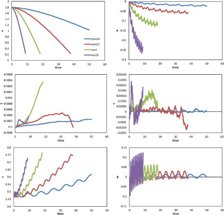
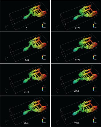
Figure 14 shows the velocity vectors and longitudinal velocity contours on the plane of during one tail-beat cycle from to for the case where with and A = 0.25. The corresponding vortex structures are shown in Figure 15. Two peaks of longitudinal velocity in the cycle can be seen in Figure 13, and correspond approximately to the times at and (T is the period of one tail-beat cycle), when the tail was close to crossing the body's vertical central plane. A backward wake flow with oscillation is shown in Figure 14. Note that a region of high backward velocity was generated on the leeward side (facing oppositely to the direction of the swinging movement) of the tail and shed into the wake flow when the swinging movement changed directions. As the high velocity was not induced on the windward side (facing to the direction of the swinging movement), this implies that rather than by ‘pushing’ the fluid, the thrust was generated more by ‘pulling’ it. The mechanism of thrust generation can also be investigated from the perspective of vortex structure in Figure 15. A series of vortex rings are shed from the trailing edge of the tail to form a reverse Karman vortex street in the wake flow, which, upon reaching the walls, moved backward along them. The body component of the model was surrounded by weak vortex structures while no obvious shedding of body vortex was observed.

Figure 14. Velocity vectors and color contours of velocity in one cycle for the case of with and A=0.25.

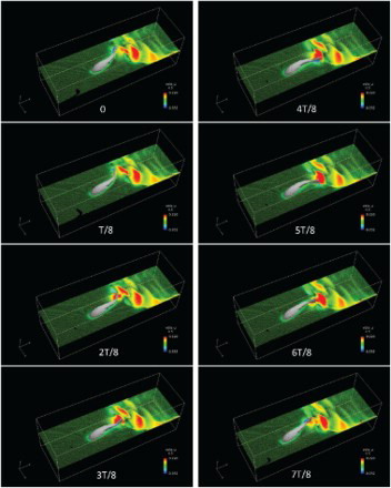
Figure 15. Vortex structures visualized according to the second invariant of the velocity-gradient tensor in one cycle for with and A = 0.25.

In addition to the tail-beat frequency, another important factor that significantly affects the swimming performance is the undulatory mode, of which anguilliform and carangiform are common types (Gillis, 1996; Sfakiotakis et al., 1999). For different undulatory modes, the propulsive wavelength can be different. The smallest propulsive wavelength for a species decreases with increasing number of vertebrae (Long & Nipper, 1996). In this study, as the number and size of the segments of the model were fixed, the relative phase difference was altered to change the undulatory mode, and its effect on swimming performance was investigated. Figure 16 compares the displacement (left) and velocity components (right) against time along the three directions for , and pi, with and A = 0.25. As the phase difference increased, the longitudinal swimming distance to the initial position decreased, except in cases where and , for which the swimming distance was slightly larger than that for and , respectively. 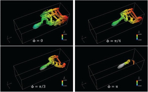When the phase difference was greater than , there was no apparent displacement along any direction. By comparing the peak-to-peak height, stronger oscillations for the longitudinal and lateral velocities were obtained when the phase differences were smaller. This indicated that more intense acceleration and deceleration process occurred in a mode where the fish body was ‘stiffer’, and this corresponded to higher swimming velocity. Figure 17 shows the vortex structures for , with and A = 0.25. As the phase difference increased, the backward jet flow weakened and fewer vortex structures were observed, especially when , where the tail plane was always parallel to the vertical central plane of the body and swung in a narrow region. It is noteworthy the proposed fish model has only four rotation joints, which may not be adequate to express the features of certain swimming patterns, especially those with larger phase differences. It is thought that models with more and smaller segments are needed to better represent large phase differences, or smaller propulsive wavelengths.

Figure 16. Profiles of the displacement (left) and velocity component (right) against time along three directions for different phase differences ( and A = 0.25).

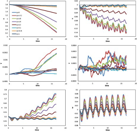
Figure 17. Vortex structures for and A = 0.25.

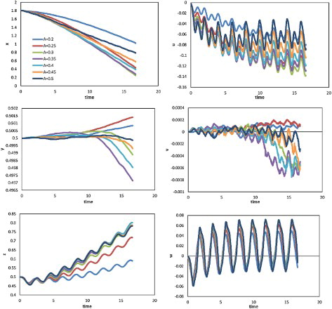
To illustrate the effect of body amplitude, Figure 18 shows the displacement (left) and corresponding velocity components (right) against time in three directions for values of parameter A ranging from 0.2 to 0.5 for constant and . As can be seen, the largest longitudinal displacement is obtained when A is between 0.3 and 0.35, while the oscillation of longitudinal velocity increases for larger body amplitudes. The swimming velocity appears to be sensitive to the body amplitude in a narrow range. The lateral displacement and velocity changes, and a slight peak shoulder appears in the lateral velocity profile, when A is larger than 0.3. Note that, unlike with the tail-beat frequency or phase difference, stronger oscillation may occur even at a lower longitudinal velocity when changing the amplitude. When the amplitude is higher than the optimal value (where the largest mean longitudinal velocity is obtained), the peak-to-peak height of the longitudinal velocity increases, while the swimming rate decreases. This implies a decrease of swimming efficiency as the amplitude increases, and requires further investigation. Because of the plane symmetry of the model and the lack of manipulation of swimming stability and direction, the vertical movement was unstable. The tail-beat frequency and phase difference were fixed to focus on the effect of body amplitude, and it should be noted that swimming performance depends on a combination of many factors rather than a single one. Thus, the optimal amplitude may change under different conditions, and this also requires further study.

Figure 18. Profiles of the displacement (left) and velocity component (right) against time along three directions for the cases with different body amplitudes ( and ).

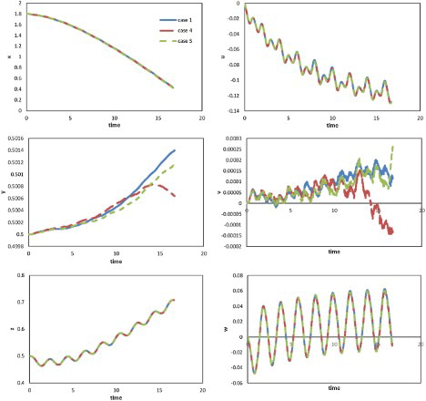
In this study, the boundary conditions were set as non-slip walls along the vertical and lateral directions, and the vortex was thus confined to the channel and could not diffuse into the far field. This was different from the normal condition such as swimming in a river or ocean where the flow field is considerably wider than the channel. Therefore, to assess the effects of the limitations imposed by the walls on swimming performance, simulations using enlarged grids were carried out. For the lateral direction, two cases (Cases 2 and 3) were examined with grids expanded along the lateral direction, with double width for Case 2 and triple width for Case 3. Meanwhile, for the vertical direction, Cases 4 (double height) and 5 (triple height) with grids expanded along the vertical direction were examined. We used Case 1 as the aforementioned case of width = 1, with parameters A = 0.25, and . These initial conditions were retained for Cases 2, 3, 4, and 5. The displacements and velocity components against time in Cases 1, 2, and 3 are compared in Figure 19, the results of Cases 1, 4, and 5 are shown in Figure 20. From Figure 19, the effect of the distance between the lateral walls on swimming performance was shown to be insignificant along all three directions. Figure 20 showed that the effect of the channel height was also insignificant, although instability in the vertical direction was observed. The relatively low Reynolds number in this study may account for the absence of significant reflection from the wall. Meanwhile, even though an additional drag component arose due to the wall, it may be offset to some extent by increasing thrust.

Figure 19. Profiles of displacements (left) and velocity components (right) against time along three directions for the cases using grids of different widths.

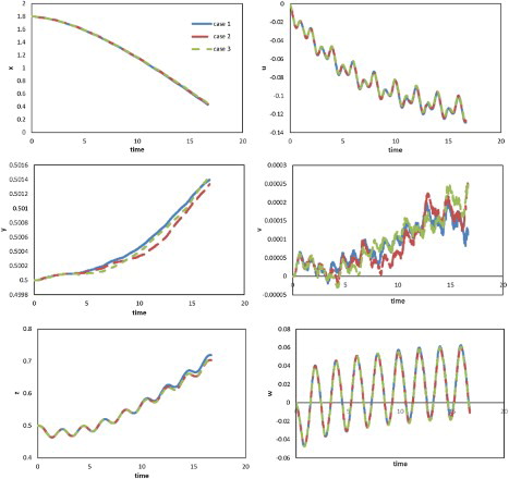
Figure 20. Profiles of displacements (left) and velocity components (right) against time along three directions for the cases using grids of different heights.

Conclusions

A 3D numerical simulation of a self-propelled fish-like object swimming in a channel with non-slip wall conditions specified along the lateral and vertical directions was conducted. The moving body was generated by employing the immersed boundary method. A parametric study was performed to investigate the effects of the tail-beat frequency, phase difference, and body amplitude on virtual swimming performance. The above results verified the feasibility and effectiveness of the simulation. The details of the flow field can help gain a better understanding of the swimming mechanisms and designs of artificial underwater machines, such as robotic fish. Differences in swimming performance in various swimming modes highlighted the effect of each parameter and implied the reasonability of the swimming forms in real fish. The below conclusions can be drawn from the results of the study.

Swimming velocity increases approximately linearly with tail-beat frequency. This relationship has been indicated in some previous studies, and it was examined using the present self-propelled settings. Wake vortices shed from the tail and formed a reverse Karman vortex street, which played an important role in thrust generation. There were two peak values of longitudinal velocity in the tail-beat cycle corresponding to the period when the tail crossed the vertical central plane of the body.

Results obtained for various phase differences among neighboring rigid body parts show that swimming was more efficient with a small phase difference than with a large one. It needs to be pointed out that the model used here may need to be modified with more segments to better express undulatory modes in large phase differences.

There exists an optimal body amplitude to obtain a maximum average longitudinal velocity when the other two parameters (frequency and phase difference) are fixed. As the amplitude increases, the oscillation of longitudinal velocity increases while the difference in lateral velocity is not significant when the amplitude is larger than the optimal value. The discrepancy between the changing tendencies of the oscillation and translational movement in the longitudinal direction as the amplitude increases implies a decrease of swimming efficiency. The fluctuation in vertical velocity implies the importance of pectoral fins on the stability of swimming.

By comparing the cases using grids of different widths or heights, the effect of the lateral and vertical wall distance on swimming performance was shown to not be significant. This implies that the above conclusions may also be applicable to swimming in a wider field, thus avoiding a requirement for greater computational cost.

There are some limitations to this study, such as the simplification of the fish body and dynamic modeling. At the same time, the main parameter concerning swimming performance here is velocity. Some other aspects such as energy efficiency were not discussed, but should be addressed in future work. Furthermore, although cases involving different simulation fields showed that the effect of lateral or vertical wall distance was not significant, further examination of the boundary effect is needed.

Disclosure statement

No potential conflict of interest was reported by the authors.

References

- Anderson, J. M., Streitlien, K., Barrett, D. S., & Triantafyllou, M. S. (1998). Oscillating foils of high propulsive efficiency. Journal of Fluid Mechanics, 360, 41–72. doi: 10.1017/S0022112097008392
- Balaras, E. (2004). Modeling complex boundaries using an external force field on fixed Cartesian grids in large-eddy simulations. Computers & Fluids, 33, 375–404. doi: 10.1016/S0045-7930(03)00058-6
- Barrett, D. S., Triantafyllou, M. S., Yue, D. K. P., Grosenbaugh, M. A., & Wolfgang, M. J. (1999). Drag reduction in fish-like locomotion. Journal of Fluid Mechanics, 392, 183–212. doi: 10.1017/S0022112099005455
- Beal, D. N., Hover, F. S., Triantafyllou, M. S., Liao, J. C., & Lauder, G. V. (2006). Passive propulsion in vortex wakes. Journal of Fluid Mechanics, 549, 385–402. doi: 10.1017/S0022112005007925
- Borazjani, I., Ge, L., & Sotiropoulos, F. (2008). Curvilinear immersed boundary method for simulating fluid structure interaction with complex 3D rigid bodies. Journal of Computational Physics, 227, 7587–7620. doi: 10.1016/j.jcp.2008.04.028
- Borazjani, I., & Sotiropoulos, F. (2008). Numerical investigation of the hydrodynamics of carangiform swimming in the transitional and inertial flow regimes. The Journal of Experimental Biology, 211, 1541–1558. doi: 10.1242/jeb.015644
- Borazjani, I., & Sotiropoulos, F. (2010). On the role of form and kinematics on the hydrodynamics of self-propelled body/caudal fin swimming. The Journal of Experimental Biology, 213, 89–107. doi: 10.1242/jeb.030932
- Braza, M., Chassaing, P., & Minh, H. H. (1986). Numerical study and physical analysis of the pressure and velocity fields in the near wake of a circular cylinder. Journal of Fluid Mechanics, 165, 79–130. doi: 10.1017/S0022112086003014
- Epps, B. P., Alvarado, P. V. y., Youcef-Toumi, K., & Techet, A. H. (2009). Swimming performance of a biomimetic compliant fish-like robot. Experiments in Fluids, 47, 927–939. doi: 10.1007/s00348-009-0684-8
- Fauci, L. J., & Peskin, C. S. (1988). A computational model of aquatic animal locomotion. Journal of Computational Physics, 77, 85–108. doi: 10.1016/0021-9991(88)90158-1
- Gillis, G. B. (1996). Undulatory locomotion in elongate aquatic vertebrates: Anguilliform swimming since Sir James Gray1. American Zoologist, 36, 656–665. doi: 10.1093/icb/36.6.656
- Hirose, T., Kihara, H., & Abe, K. (2012, November). Numerical simulation of flow field around a wing with surface oscillation using an immersed boundary method. The 90th conference of JSME fluid dynamics division, CD-ROM, Kyoto, Japan.
- Jordan, S., & Fromm, J. (1972). Oscillatory drag, lift, and torque on a circular cylinder in a uniform flow. Physics of Fluids, 15, 371–376. doi: 10.1063/1.1693918
- Kern, S., & Koumoutsakos, P. (2006). Simulations of optimized anguilliform swimming. The Journal of Experimental Biology, 209, 4841–4857. doi: 10.1242/jeb.02526
- Kim, J., Kim, D., & Choi, H. (2001). An immersed-boundary finite-volume method for simulations of flow in complex geometries. Journal of Computational Physics, 171, 132–150. doi: 10.1006/jcph.2001.6778
- Lauder, G. V., & Drucker, E. G. (2002). Forces, fishes, and fluids: hydrodynamic mechanisms of aquatic locomotion. News Physiol Sci, 17, 235–240.
- Liao, J. C. (2007). A review of fish swimming mechanics and behavior in altered flows. Philosophical Transactions of the Royal Society B: Biological Sciences, 362, 1973–1993. doi: 10.1098/rstb.2007.2082
- Liu, J., & Hu, H. (2010). Biological inspiration: From carangiform fish to multi-joint robotic fish. Journal of Bionic Engineering, 7, 35–48. doi: 10.1016/S1672-6529(09)60184-0
- Liu, H., & Kawachi, K. (1999). A numerical study of undulatory swimming. Journal of Computational Physics, 155, 223–247. doi: 10.1006/jcph.1999.6341
- Long, J. H. J. R., Mchenry, M. J., & Boetticher, N. C. (1994). Undulatory swimming: How traveling waves are produced and modulated in sunfish (Lepomis gibbosus). The Journal of Experimental Biology, 192, 129–145.
- Long, J. H. J. R., & Nipper, K. S. (1996). The importance of body stiffness in undulatory propulsion. American Zoologist, 36, 678–694. doi: 10.1093/icb/36.6.678
- Luo, K., Wang, Z., & Fan, J. (2007). A modified immersed boundary method for simulations of fluid-particle interactions. Computer Methods in Applied Mechanics and Engineering, 197, 36–46. doi: 10.1016/j.cma.2007.07.001
- Mordant, N., & Pinton, J.-F. (2000). Velocity measurement of a settling sphere. The European Physical Journal B, 18, 343–352. doi: 10.1007/PL00011074
- Muto, M., Tsubokura, M., & Oshima, N. (2012). Negative Magnus lift on a rotating sphere at around the critical Reynolds number. Physics of Fluids, 24, 1–15. doi: 10.1063/1.3673571
- Naito, H., & Fukagata, K. (2012). Numerical simulation of flow around a circular cylinder having porous surface. Physics of Fluids, 24, 117102-1–117102-19. doi: 10.1063/1.4767534
- Narasimha, M., Brennan, M., & Holtham, P. N. (2007). A review of CFD modelling for performance predictions of hydrocyclone. Engineering Applications of Computational Fluid Mechanics, 1(2), 109–125. doi: 10.1080/19942060.2007.11015186
- Sfakiotakis, M., Lane, D. M., & Davies, J. B. C. (1999). Review of fish swimming modes for aquatic locomotion. IEEE Journal of Oceanic Engineering, 24, 237–252. doi: 10.1109/48.757275
- Stamou, A. I., Katsiris, I., Politis, M., & Schaelin, A. (2008). Applying a CFD model to evaluate thermal comfort in the MPC amphitheatre of the Olympic games “Athens 2004”. Engineering Applications of Computational Fluid Mechanics, 2(1), 41–50. doi: 10.1080/19942060.2008.11015210
- Triantafyllou, M. S., Techet, A. H., Zhu, Q., Beal, D. N., Hover, F. S., & Yue, D. K. P. (2002). Vorticity control in fish-like propulsion and maneuvering1. Integrative and Comparative Biology, 42, 1026–1031. doi: 10.1093/icb/42.5.1026
- Tritton, D. J. (1959). Experiments on the flow past a circular cylinder at low Reynolds numbers. Journal of Fluid Mechanics, 6, 547–567. doi: 10.1017/S0022112059000829
- Tseng, Y., & Ferziger, J. H. (2003). A ghost-cell immersed boundary method for flow in complex geometry. Journal of Computational Physics, 192, 593–623. doi: 10.1016/j.jcp.2003.07.024
- Wang, F., Reitz, R., Pera, C., Wang, Z., & Wang, J. (2013). Application of generalized RNG turbulence model to flow in motored single-cylinder PFI engine. Engineering Applications of Computational Fluid Mechanics, 7(4), 486–495. doi: 10.1080/19942060.2013.11015487
- Webb, P. W. (1993). The effect of solid and porous channel walls on steady swimming of steelhead trout Oncorhynchus mykiss. The Journal of Experimental Biology, 178, 97–108.
- Webber, D. M., Boutilier, R. G., Kerr, S. R., & Smale, M. J. (2001). Caudal differential pressure as a predictor of swimming speed of cod (Gadus morhua). The Journal of Experimental Biology, 204, 3561–3570.
- Wu, T. Y. (2001). Mathematical biofluiddynamics and mechanophysiology of fish locomotion. Mathematical Methods in the Applied Sciences, 24, 1541–1564. doi: 10.1002/mma.218
- Zhu, Q., Wolfgang, M. J., Yue, D. K. P., & Triantafyllou, M. S. (2002). Three-dimensional flow structures and vorticity control in fish-like swimming. Journal of Fluid Mechanics, 468, 1–28. doi: 10.1017/S002211200200143X