Optimization procedure for variable speed turbine design

ABSTRACT

This article outlines a design procedure for variable speed Francis turbines using optimization software. A fully parameterized turbine design procedure is implemented in MATLAB. ANSYS CFX is used to create hill diagrams for each turbine design. An operation mode of no incidence losses is chosen, and the mean efficiency in the range of the best efficiency point is used as optimization criterion. This characteristic is extracted for each design, and optiSLang is used for system coupling and optimization. In the global optimization loop, the downhill simplex method is used to maximize the turbine performance. For this article, the bounding geometry of the runner is kept as in the original configuration. This way, the performance of the different variable speed turbines can be compared directly. Two optimization parameters describing the blade leading-edge geometry have been used in the optimization procedure. The resulting design was an almost circular leading edge, and shows an increase in mean efficiency of 0.25% compared to the reference case. There was a significant change in the turbine performance, with close to no change at the best efficiency point, and an increase in efficiency of almost 1% at low rotational speed. The outlined procedure is parallelizable and can be performed within an industrial timeframe.

KEYWORDS:

• Numerical simulations
• optimization
• hydraulic turbines
• design
• CFD

1. Introduction

Modern computational resources allow Computational Fluid Dynamics (CFD) to be an integral part of turbine design. A vast amount of research has been done on numerical simulation of hydraulic turbines. A state-of-the-art review can be found in Trivedi, Cervantes, and Gunnar Dahlhaug (2016). The main take-away is that the different flow phenomena require very different modeling strategies; tip vortices require more advanced turbulence models than other phenomena, pressure pulsations need transient simulations, but simulation time can be drastically reduced by Fourier-series-based passage modeling, and importantly, global parameters can easily be obtained with steady simulations due to the periodic-in-time nature of the flow field. Within numerical simulations on hydropower, the most advanced numerical simulations include all components, use hundreds of millions of mesh elements, model water as a compressible fluid, and use sophisticated turbulence models like large eddy simulations. The accuracy of the simulations has reached excellent levels, shown e.g. by the research project Francis99 (Norwegian Hydropower Centre, 2018). Research also shows that, for global parameters such as hydraulic efficiency and head, simpler modeling assumptions give good results (Tengs, Storli, & Holst, 2018). When simulations are trusted, the natural extension of traditional design involves optimization techniques.

Optimization of hydraulic turbines is not new. Several examples of Francis turbine runner optimization exist (Enomoto, Kurosawa, & Kawajiri, 2012; Nakamura & Kurosawa, 2009; Pilev et al., 2012), some even optimizing the runner and draft tube simultaneously (Lyutov, Chirkov, Skorospelov, Turuk, & Cherny, 2015). Most of these attempts deal with medium-to-high specific speed Francis turbines, but other turbine types have also been optimized using similar techniques (Ezhilsabareesh, Rhee, & Samad, 2018; Semenova et al., 2014). The peak efficiency of hydro turbines has not increased much in the last decades, as noted in Electric Power Research Institute (1999) and Lyutov et al. (2015). Instead, optimization attempts usually aim to increase the efficiency away from the best operating point. Typically, one point at part load and one point at high load are chosen.

Recent changes in the international power market and the introduction of intermittent power sources have led to increased demand from hydro turbines. The operation of turbines has changed to more off-design operation, which results in lower efficiencies and higher wear. One solution to this problem is to make variable speed turbines, a technology that allows a turbine to operate in a larger operating range without increased fatigue wear. The idea of using variable speed is not new. Back in 1987, several turbine types were tested to investigate if variable speed could increase performance (Farell & Gulliver, 1987). More recent investigations into variable speed utilize computational tools and show the possibility of increasing the efficiency at off-design conditions (Abubakirov et al., 2013). Power plants with large variations in head will also gain from variable speed operation, as seen in Pérez, Wilhelmi, and Maroto (2008). Today, most variable speed units are reversible pump–turbines (Energy Storage Association, 2018). This article introduces a simulation and optimization framework for the design of variable speed turbines. The optimization procedure is based on the two-dimensional hill diagram of a variable speed Francis turbine. The optimization objective is taken from a number of operating points along a line in the operating space with small incidence losses. Structural performance, draft tube phenomena, etc. will not be covered in this article.

2. Theory and methods

2.1. Conventional and variable speed operation of Francis turbines

An hydraulic turbine converts the available static pressure energy in a water body into torque and rotational energy in the runner. The static pressure in pascals is given by (1) where ρ kg is the water density and H metres is the height of the water column above the turbine. The potential power, P watts, in the water body can then be expressed as , where Q m³/s is the volume flow. The rotational output power in the runner can be expressed as the torque, T newton-metres, multiplied by the rotational speed, ω hertz, and as it is impossible to extract all the potential energy from the water, an hydraulic efficiency can be defined as follows: (2)

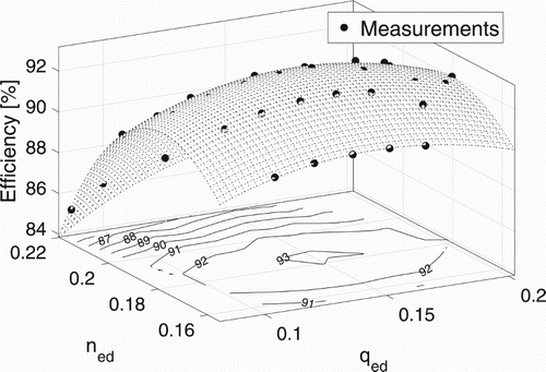
The hydraulic efficiency of a modern Francis turbine can exceed 96% at the best operating point (Andritz Hydro, 2018). At off-design conditions, however, the efficiency will be lower due to incidence losses at the inlet, spin losses at the outlet, etc. The hill diagram is used as a visual representation of how the efficiency changes. Assuming a test plant where both the flow rate and the runner speed are adjustable, if the hydraulic efficiency is measured at various points in the operational space and plotted, the resulting surface will form a convex hill, with the best operation point (ideally) at the top. A hill diagram is a two-dimensional projection of such a surface. The general idea is presented in Figure 1. The axes are normalized versions of the flow rate, Q, and rotational speed, n, see Equations (3(3) ) and (4(4) ), where D meters is the runner diameter (Dörfler et al., 2012). This formulation allows for easier comparison between different turbines. (3) (4)

Figure 1. Example hill diagram: a 2D projection of a 3D surface.

Conventional hydro turbines operate at a fixed speed controlled by the frequency of the power grid. The guide vanes allow for adjustment of the mass flow through the runner, and the hydraulic efficiency can be displayed as a function of the flow rate or guide vane opening only. In a variable speed turbine, however, both the runner speed and the flow rate are adjustable. This allows the turbine operator to match the runner speed and guide vane opening such that the water entering the runner perfectly coincides with the runner geometry. This could reduce the aforementioned incidence losses at off-design operation. In terms of bounding geometry, there is no difference between a runner installed in a variable speed turbine and one installed in a conventional hydro turbine. However, from an optimization point of view, it is obvious that the desired characteristics from a hill diagram are different. In a conventional runner, the efficiency need only be optimized in one dimension (the flow rate), whereas a two-dimensional representation is required for a variable speed turbine.

2.2. The optimization procedure

The idea is to design turbines using a Francis-runner design tool, create hill diagrams for the different designs, analyse the hill diagrams, and couple them all together in an optimization loop. The goal is to end up with a variable speed turbine design. The optimization procedure is presented in Figure 2. The procedure is similar to that presented in Ezhilsabareesh et al. (2018) and Jiang et al. (2018), although applied on a different turbine type. The following sections will describe the different blocks presented in Figure 2 in some detail, and how they interact.

Figure 2. Optimization loop based on hill diagrams.

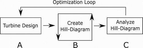
2.2.1. Block A – turbine design

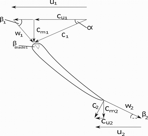
Traditional turbine design is a combination of using the Euler turbine equations and empirical knowledge. The procedure outlined here is adapted from the works of Brekke (2003). In order to describe the design steps of a Francis turbine, we need to define some nomenclature. The rated water head, H, and flow rate, Q, are known in advance. The velocity components entering and exiting a typical blade are shown in Figure 3. The letter u (m/s) denotes the runner velocity, c (m/s) denotes the water absolute velocity, and w (m/s) denotes the water velocity relative to the runner. The guide vane angle, , is controlling the angle of the water entering the runner, and thus implicitly also , the angle of the water in the rotating frame of reference. The subscripts u and m denote the tangential and meridional directions, respectively, and the subscripts 1, 2 denote the inlet and outlet. The meridional velocity component is the component in the flow direction, i.e. .

Figure 3. Velocity components on runner blade.

Before defining the main dimensions of the turbine, we use the Euler turbine equation (Subramanya, 2013) to derive an important relation: (5)

The second term in Equation (5(5) ) will contribute purely negatively to the efficiency, therefore this term is set to zero at optimum design. As is the runner velocity, and strictly non-zero, this equates to setting (6)

Physically, this condition means is that there should be no spin in the water body at the outlet. The turbine should transfer all the rotational energy in the water over to the runner. This condition will be used throughout the following derivation. It is customary to start designing a turbine from the outlet. Two parameters are chosen in advance, and. Based on empirical knowledge, these parameters are taken from the following range (Gogstad, 2012): (7) (8) with higher values corresponding to higher head. Once the above parameters are chosen, the meridional outlet velocity can be calculated (keeping in mind Equation 6(6) ): (9)

The outlet radius is then easily derived: (10) where  m² is the outlet area. Once the outlet dimension is set, the rotational speed of the turbine is calculated as follows: (11) where ω and n is the rotational speed in hertz and r.p.m. In general, n will not be the synchronous speed, which is a requirement in conventional turbines. To change this, the closest synchronous speed is chosen, and the design process of Equations (9(9) )–(11(11) ) is repeated in reverse order. This is strictly not necessary for variable speed turbines. Once the outlet dimensions are set, the inlet is designed. As for the outlet, an empirical range is used, this time for the runner inlet velocity: (12) where the overbar notation denotes a reduced parameter: (13)

The inlet radius is now given directly by the runner speed, and the inlet runner velocity: (14)

The meridional velocity can be found by demanding that the velocity through the runner is increasing. This will reduce the chance for flow separation, backflow, and other phenomena in the runner. A typical acceleration is 10%, i.e. (15)

The height of the inlet channel, B metres, is then found by (16)

Finally, the inlet blade angle, , needs to be calculated. From Figure 3 we see that the inlet tangential water velocity is needed. Returning to the Euler turbine equation, (17)

With , Equation (5(5) ) reduces to , and as the runner speed is set, this allows for calculation of the tangential water velocity component: (18) with being a typical value (Brekke, 2003). This is because 100% efficiency is impossible due to hydraulic friction, bearing losses, etc. As the final main parameter, can be calculated as (19)

When the main parameters are set, further details need to be determined. From the Euler turbine equation, Equation (5(5) ), we see that the quantity is a measure of energy. From Equation (6(6) ) we also see that this quantity is zero at the outlet . How the distribution changes through the runner is free for the designer to choose. Typically, the - distribution is chosen such that most of the energy is transferred to the runner in the beginning of the runner. This is due to runner blades generally being thinner and more prone to fractures at the outlet. The blades will also be given a thickness distribution, and leading and trailing edge profiles. These modifications will change the flow area in the runner channels, and in general one should revert back to Equations (10(10) ) and (16(16) ) to account for this. The design procedure outlined here is implemented in a MATLAB code. The program writes the turbine geometry into text files that are compatible with the ANSYS software.

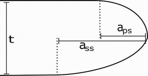
In terms of optimization, there exist tens of free optimization parameters: number of blades, energy distributions, thickness distributions, leading and trailing edge shape, etc. In this article, only two parameters, as listed in Table 1 and shown in Figure 4, have been chosen. The parameters define the leading-edge geometry of the blade. Both the pressure and suction sides of the leading edge are expressed as ellipses, and the parameters , control the free axis in the ellipses, as the blade leading edge thickness in this case is held constant at  mm. Changing the parameters changes the curvature of the leading edge, and presumably also the turbine performance at different operating conditions, i.e different inlet flow angles.

Table 1. Optimization parameters.

Parameters	Type	Range (mm)
, pressure side geometry	Continuous	10–40
, suction side geometry	Continuous	10–40

Figure 4. Definition of leading edge geometry.

The reason only these parameters are chosen is twofold: the main goal of this article is to prove that the optimization framework works. This is best shown using few parameters so that the simulation time is in a reasonable range. Secondly, it is desired to use parameters where the bounding runner geometry is unchanged. This way, the different designs can be compared directly. For reference, the main dimensions in all the runners in this article are the following: H=350 m, Q=25 m³/s, ,  m and  m. The specific speed is , classifying this as a high-head Francis turbine. The - distribution through the runner follows the relation , where x=1 marks the inlet and x=0 the outlet.

2.2.2. Block B – simulation

Block B contains an ANSYS Workbench project, where the geometry is meshed in TurboGrid, and simulated in CFX. The present authors have previously published an article on the accuracy and time-consumption of a numerically simulated hill diagram (Tengs et al., 2018). Some of the results will be repeated here. The Norwegian University of Science and Technology provided an experimentally obtained hill diagram along with a model geometry. About 40 operating points were simulated, and the experimental data were used as validation. The guide vane opening and the runner speed were operated in the range and , respectively, of the assumed best efficiency point. ANSYS CFX was used for simulation, as this is the leading simulation software with regards to rotating machinery. Only the runner domain and a cut-off draft tube were simulated, this ensured that only one mesh was needed for the whole hill diagram. In the runner domain, one passage was simulated, utilizing the rotational symmetry of the geometry. The different operating points were tested by changing the direction of the velocity components on the inlet, the mass flow, and the runner speed. The simulation strategy of no re-meshing allowed for parallel simulation of all operating points. Steady state, passage modeling, and incompressible flow were assumed to reduce the simulation time where possible. 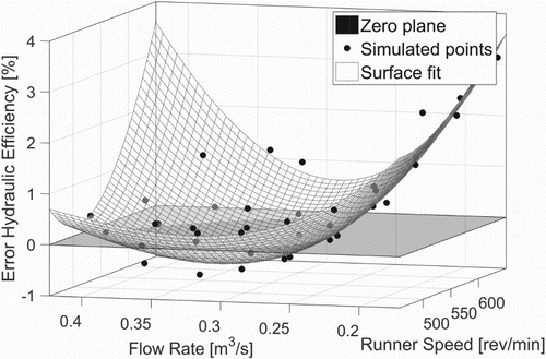The SST turbulence model was used, and the average in the runner was 2.8. Mesh convergence was confirmed using the GCI method due to Celik, Ghia, Roache, and Christopher (2008). The boundary condition at the inlet was the mass flow taken from the experiment; at the outlet, zero relative pressure was used. The results were highly encouraging. If one disregards operating points with extremely low guide vane opening, the error in hydraulic efficiency was found to be less than 2.5% in the whole simulated range. Around the best efficiency point, the deviation was in the order of 0.5%, see Figure 5. The error was also not randomly distributed, but followed a clear pattern. The simulations were performed on a workstation using 6 cores in parallel, and each simulated point took approximately 15 minutes. Using more powerful hardware, or utilizing the parallelization properties of the method, could decrease the simulation time drastically.

Figure 5. Error in hydraulic efficiency, taken from Tengs et al. (2018).

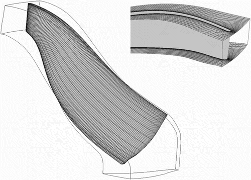
Based on the above, a numerically obtained hill diagram is assumed to be trusted, especially for identifying behavioural trends. This is based on the non-random error distribution of the simulated head and torque (Tengs et al., 2018). Far away from the best efficiency point, simulation error is inevitable; however, the error is assumed to behave equally in all designs, making a relative comparison valid. Similar simulation settings as in the reference are used in this article, however expanded to include automatic meshing of the new runner geometry as well as the draft tube. Another necessary change is to use total pressure inlet conditions, as the mass flow is not given a priori in the simulations. The outputs of the simulation are thus the hydraulic efficiency and mass flow. The mesh was automatically generated with TurboGrid for each design; a typical blade surface mesh and inlet are shown in Figure 6. Note that the extended inlet section and draft tube is omitted for clarity. The total number of mesh elements was per passage, equivalent to 4.2 million elements if the whole turbine had been simulated rather than using passage modeling.

Figure 6. Typical mesh used in the simulations.

2.2.3. Block C – analysis

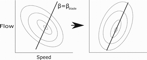
Block C defines the optimization objectives in the loop. There are many ways of analyzing the simulation output; the goal could be a high peak hydraulic efficiency, or conversely a ‘flatter’ curve, albeit with a lower peak performance. In terms of variable speed turbines, it might be clever to synchronize the flow and runner speed such that the direction of the water entering the runner matches the runner geometry. This equates to in Figure 3. This should in general result in smaller incidence losses, fewer transient effects, and better turbine operation. A high mean efficiency along this ‘line of operation’ could be an optimization criterion. Figure 7 illustrates such an approach. In this single-objective function, all operating points are given the same importance/weight; if this were a real optimization case for a customer, a weight function based on actual turbine operation should be provided. More advanced objective functions including curvature of the hill diagram, etc., is just as easily implemented; however, the mean is chosen here.

Figure 7. Optimize efficiency along line of small incidence losses.

If it were possible to input to the simulations, there would be no need to simulate the complete hill diagram. Some flow/speed combinations will not be used, and are therefore not of interest. This would in turn result in fewer simulations, and faster optimization. The problem with this approach is that it is difficult to input in the simulations. β is defined as , and since and the flowrate is not specified in the simulations, beta cannot be precisely determined in advance. Optimization along a line is still possible; however, a more ‘complete’ hill diagram is needed, assuming several operating points have been simulated. The flow rate can now be plotted with respect to guide vane opening and runner speed. By using a surface fitting procedure, one can obtain a mathematical description of this relation, . Thus, the inlet angle can be reduced to a function of the inlet parameters only: (20)

Such an approach was implemented in MATLAB. The runner speed and guide vane angle were simulated in a matrix for each design. The limits were set to ±30% of the assumed optimal configuration for both input values. A complete second order fit was performed on the resulting mass flow versus speed and α; β was then calculated from Equation 20(20) , and the hydraulic efficiency was extracted at five points along a line where . 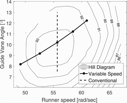Finally, the mean efficiency of the five points was used as optimization characteristic. The above algorithm was tested on the experimental data from the hill diagram validation case mentioned in Section 2.2.2. The guide vane angle/runner speed combinations with β equal to that of the best operating point was found and plotted together with the hill diagram in Figure 8. A line indicating the conventional fixed-speed operation is also included to illustrate the difference in the two operation schemes. In this example, the optimization characteristic, the mean of the five points, is.

Figure 8. Difference in operating schemes.

2.3. Optimization

Optimization is a scientific field of its own, with a vast amount of research. Surrogate models are very popular, the most known being the classical Response Surface Method (RSM) (Box & Wilson, 1992). In the RSM, the variable space is properly sampled, using Box–Behnken, Central Composite Design or similar, then the outcomes are evaluated and a surrogate model is created based on the results. This allows for the possibility of creating meta-models/reduced order models of a process response, and makes the method very popular. Similar methods have also been used in the turbine industry (Enomoto et al., 2012; Ezhilsabareesh et al., 2018). Another, newer, optimization strategy is the evolutionary algorithm. The method mimics biological populations; a randomly sampled parameter set evolves in a fashion similar to how populations evolve through generations (Jiang et al., 2018; Vikhar, 2016). Recently, artificial/computational intelligence (CI) or machine learning methods have received much attention; e.g. in Kazemi et al. (2018) and Ardabili et al. (2018), 21 articles from the present decade regarding the usage of CI in the hydrogen production industry alone are reviewed. The mentioned methods are global methods, and fairly computationally expensive. A more classical approach employs gradient based methods, e.g. the conjugate gradient method (Hestenes & Stiefel, 1952). In essence, these methods find the gradient of the response and ‘move’ in the desired direction (i.e. maximize a function). These methods are not a global methods, meaning the final solution may be a local optimum rather than the global one. However, such methods will find an approximate optimum fairly fast. Finally, there is a branch of optimization techniques called local search, including the hill-climbing method and the simplex method (Nelder & Mead, 1965). Common to these methods is making small local changes in the variables, and a direct evaluation of the new response. As with gradient based methods, these methods are not global.

The commercial software optiSLang has been used to couple all the blocks presented in Figure 2 together. optiSLang is an optimization software based on graphical programming, where external programs can be used as modules in a system. In this case, MATLAB and ANSYS have been the different modules. The program can automatically select the appropriate optimization algorithm from among gradient methods, evolutionary strategies, adaptive response surface method (ARSM), etc. Which methodology is used is very much dependent on the problem at hand, and the time needed for the evaluation of each outcome. In this article, the simplex method will be used, owing to its simplicity.

2.3.1. Downhill simplex method

The downhill simplex method is a non-gradient-based method. It is, however, not a global method, and the solution does therefore in general risk getting caught in a local optimum. For a small number of optimization parameters, the convergence is fast. For a larger number, other algorithms may be preferred. The method is chosen here owing to its simplicity. The simplex method starts of by creating a geometrical figure (a simplex) of N+1 vertices, with N being the number of optimization parameters. The vertex values are evaluated, before simple transformations (reflection, expansion, contraction) are applied to the simplex, to obtain new design points to be evaluated. In this way, the solution progresses towards the optimum. A thorough explanation can be found in the original article by Nelder and Mead (1965). In summary, the downhill simplex method will be used to optimize the leading-edge geometry of a Francis turbine runner. The optimization goal is to maximize the mean hydraulic efficiency along a line of small incidence losses, as presented in Section 2.2.3.

3. Results

The results from the optimization procedure are presented in Table 2. We observe that the converged solution is well within the given parameter range. Throughout the results section, designs 5 and 24 will be used as representatives for designs early and late in the optimization process, respectively. The first few designs are avoided because the initial guess was chosen arbitrarily. Figure 9 shows the change in the leading edge geometry (please refer to Figure 4 for definitions).

Figure 9. Comparison between one of the earlier and one of the final designs, i.e. 5 and 24, respectively.

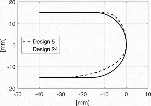
Table 2. Optimization results.

Method	Result []
Downhill simplex	[14.06, 16.15]

The optimization algorithm was manually terminated after 28 iterations following a visual inspection of the convergence. Figure 10(a) shows the convergence of the simplex algorithm. The y-axis shows the mean efficiency relative to the maximum mean efficiency. We see a difference of in the mean efficiency in the different designs. The increase is significant when such a limited parameter set is considered.

Figure 10. Change in performance as the simplex method is converging to the final design.

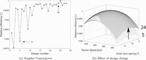
The objective function in this article is the mean, and no information is thus provided as to how the hill-diagram shape changes. Figure 10(b) is therefore included to show the hill diagram of designs 5 and 24, with the z-axis being the efficiency relative to the best efficiency. We see that, around the best operating point, there are no significant variations; however, at low runner speed and small guide vane opening, the performance differs by more than 0.5%.

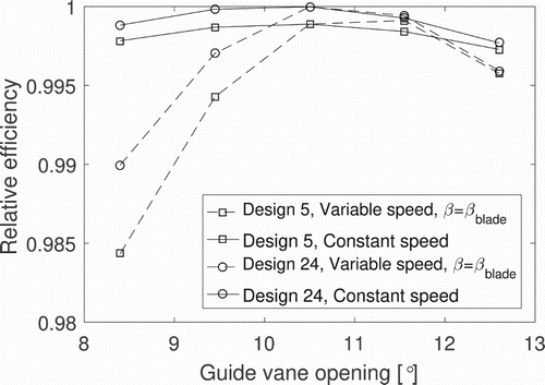
It should be noted that the assumption that the best operation mode is along is not necessarily valid, at least not for the designs tested here. By operating the new design as a conventional runner (constant speed), the mean efficiency will be larger than if is satisfied. The optimized design performs better than the start design in both operation modes. See Figure 11 for comparison of designs 5 and 24 (variable speed is denoted by dashed lines). The different operation modes are shown in Figure 8. The reason why conventional operation is superior is that, when only the leading edge geometry is changed, the different turbines will still be very similar. The design from Section 2.2.1 is unchanged, the thickness of the blades is the same, etc. Keeping in mind that the original turbine was designed for constant speed, then conventional operation is therefore more efficient. There are a number of other design parameters that could trigger larger changes in the hydraulic efficiency and be more interesting from a design point of view. In essence, to get a proper, optimized, variable speed turbine, more parameters have to be included in the optimization loop.

Figure 11. Efficiency along different lines of operation.

4. Discussion and further work

The simulations in this article were performed on a laptop using four cores in parallel. The simulation of each hill diagram took about two hours. The time used on design and post-processing was negligible, meshing and simulation in ANSYS accounting for all time consumption. By using hardware with more cores, the simulation time per hill diagram could be significantly reduced. ANSYS reports scaling properties of efficiency for additional cores (ANSYS, 2018), a close-to-linear reduction of simulation time. Another way of drastically speeding up the simulation would be to simulate the different points in the hill diagram in parallel, as the mesh is the same. This will give a linear reduction factor equal to the number of simultaneously simulated operating points, and coupled with more powerful hardware this will reduce the simulation time to the order of minutes per hill diagram.

The simplex algorithm was terminated after a visual inspection. The reasoning is that the underlying uncertainty in the simulation of the hill diagrams, and the second order approximation when calculating the relative flow angle β, makes further optimization excessive. The absolute change from iteration to iteration reached the order of 0.01% in mean efficiency before termination. Further work should verify the simplex method by using another, preferably global, optimization method, such as the ARSM due to Gary Wang, Dong, and Aitchison (2001), to see if the same leading edge geometry is obtained.

The resulting ellipse axes are  mm,  mm, see Figure 9, which means that the final leading-edge geometry is close to a circular shape, as the blade thickness is 30 mm. It is interesting, though somewhat intuitive, that a circular edge is better at dealing with velocity entering from different angles. Any definite recommendation with respect to leading edge geometry should however not be taken from these results, as this article is a test to prove the optimization concept. As a reference, a high-fidelity simulation could be performed to reveal the actual hydraulic performance. If we do, however, assume that the result is correct, then another conclusion is that the efficiency is not very dependent on the leading-edge geometry at the best operating point. At low runner speed, however, the changes are dramatic – close to 1% increase in efficiency and a visually flatter curve. This is exactly the desired change, and indicates that the method works. The choice of using the mean as objective function, however, might not be optimal, as a flat curve is not explicitly looked for. An alternative could include, for example, the standard deviation of the points, to force a flatter curve. In future work using this framework, a more advanced analysis will be implemented.

5. Conclusions

This article presents an optimization procedure for variable speed turbines and shows that the idea of using hill diagrams as the optimization characteristic is feasible. A parametric test of the leading edge shows a mean efficiency improvement of 0.25% along a certain line of operation. At lower rotational speeds, the differences in the designs becomes more prominent, in some cases with a close to 1% efficiency increase. The actual hydraulic performance should be verified with a high-fidelity simulation. As of now, each hill diagram was created in the order of hours. The procedure is however highly parallelizable and, by utilizing this fact, the simulation time could be reduced to the order of minutes. If this is done, several parameters could be added to the optimization and the procedure still be performed within an industrial timeframe.

Disclosure statement

No potential conflict of interest was reported by the authors.

ORCID

Erik Tengs http://orcid.org/0000-0001-8873-724X

Additional information

Funding

This work was supported by Norges Forskningsråd [grant number 254987].

References

- Abubakirov, S. I., Lunatsi, M., Plotnikova, T., Sokur, P., Tuzov, P. Y., Shavarin, V., … Shchur, V. (2013). Performance optimization of hydraulic turbine by use of variable rotating speed. Power Technology and Engineering, 47 (2), 102–107. doi: 10.1007/s10749-013-0405-6
- Andritz Hydro. (2018). Turbines for hydropower plants. Retrieved from http://energystorage.org/energy-storage/technologies/variable-speed-pumped-hydroelectric-storage
- ANSYS. (2018). HPC for uids. Retrieved from https://www.ansys.com/products/fluids/hpc-for-fluids
- Ardabili, S. F., Naja_, B., Shamshirband, S., Minaei Bidgoli, B., Deo, R. C., & Chau, K.-w. (2018). Computational intelligence approach for modeling hydrogen production: A review. Engineering Applications of Computational Fluid Mechanics, 12 (1), 438–458. doi: 10.1080/19942060.2018.1452296
- Box, G. E., & Wilson, K. B. (1992). On the experimental attainment of optimum conditions. In Breakthroughs in statistics: Foundations and basic theory (pp. 270–310). New York: Springer.
- Brekke, H. (2003). Pumper & turbiner. Vannkraftlaboratoriet, Norges Teknisk-Naturvitenskapelige Universitet (NTNU).
- Celik, I., Ghia, U., Roache, P., & Christopher. (2008). Procedure for estimation and reporting of uncertainty due to discretization in CFD applications. Journal of Fluids Engineering, 130 (7), Article ID 078001. doi:10.1115/1.2960953
- Dörer, P., Sick, M., & Coutu, A. (2012). Flow-induced pulsation and vibration in hydro-electric machinery: Engineer's guidebook for planning, design and troubleshooting. London: Springer-Verlag. doi:10.1007/978-1-4471-4252-2
- Electric Power Research Institute (EPRI). (1999). EPRI Hydro life extension modernization guide, Vol. 2 – Hydromechanical equipment.
- Energy Storage Association (ESA). (2018). Variable speed pumped hydroelectric storage. Retrieved from http://energystorage.org/energy-storage/technologies/variable-speed-pumped-hydroelectric-storage
- Enomoto, Y., Kurosawa, S., & Kawajiri, H. (2012). Design optimization of a high speci_c speed Francis turbine runner. IOP Conference Series: Earth and Environmental Science, 15 (3), Article ID 032010. doi:10.1088/1755-1315/15/3/032010
- Ezhilsabareesh, K., Rhee, S. H., & Samad, A. (2018). Shape optimization of a bidirectional impulse turbine via surrogate models. Engineering Applications of Computational Fluid Mechanics, 12 (1), 1–12. doi: 10.1080/19942060.2017.1330709
- Farell, C., & Gulliver, J. (1987). Hydromechanics of variable speed turbines. Journal of Energy Engineering, 113 (1), 1–13. 25 doi: 10.1061/(ASCE)0733-9402(1987)113:1(1)
- Gary Wang, G., Dong, Z., & Aitchison, P. (2001). Adaptive response surface method – a global optimization scheme for approximation-based design problems. Engineering Optimization, 33 (6), 707–733. doi: 10.1080/03052150108940940
- Gogstad, P. J. (2012). Hydraulic design of Francis turbine exposed to sediment erosion (Master's thesis). Norwegian University of Science and Technology (NTNU).
- Hestenes, M. R., & Stiefel, E. (1952). Methods of conjugate gradients for solving linear systems. Journal of Research of the National Bureau of Standards, 49 (6), 409–436. doi: 10.6028/jres.049.044
- Jiang, J., Cai, H., Ma, C., Qian, Z., Chen, K., & Wu, P. (2018). A ship propeller design methodology of multi-objective optimization considering uid–structure interaction. Engineering Applications of Computational Fluid Mechanics, 12 (1), 28–40. doi: 10.1080/19942060.2017.1335653
- Kazemi, S., Minaei Bidgoli, B., Shamshirband, S., Karimi, S. M., Ghorbani, M. A., Chau, K.-w., & Kazem Pour, R. (2018). Novel genetic-based negative correlation learning for estimating soil temperature. Engineering Applications of Computational Fluid Mechanics, 12 (1), 506–516. doi: 10.1080/19942060.2018.1463871
- Lyutov, A. E., Chirkov, D. V., Skorospelov, V. A., Turuk, P. A., & Cherny, S. G. (2015). Coupled multipoint shape optimization of runner and draft tube of hydraulic turbines. Journal of Fluids Engineering, 137 (11), Article ID 111302. doi:10.1115/1.4030678
- Nakamura, K., & Kurosawa, S. (2009). Design optimization of a high speci_c speed Francis turbine using multi-objective genetic algorithm. International Journal of Fluid Machinery and Systems, 2 (2), 102–109. doi: 10.5293/IJFMS.2009.2.2.102
- Nelder, J. A., & Mead, R. (1965). A simplex method for function minimization. The Computer Journal, 7 (4), 308–313. doi: 10.1093/comjnl/7.4.308
- Norwegian Hydropower Centre (NVKS). (2018). The Francis99 research project. Retrieved from https://www.ntnu.edu/nvks/francis-99
- Pérez, J. I., Wilhelmi, J. R., & Maroto, L. (2008). Adjustable speed operation of a hydropower plant associated to an irrigation reservoir. Energy Conversion and Management, 49 (11), 2973–2978. doi: 10.1016/j.enconman.2008.06.023
- Pilev, I. M., Sotnikov, A. A., Rigin, V. E., Semenova, A. V., Cherny, S. G., Chirkov, D. V., … Skorospelov, V. A. (2012). Multiobjective optimal design of runner blade using e_ciency and draft tube pulsation criteria. IOP Conference Series: Earth and Environmental Science, 15 (3), Article ID 032003. doi:10.1088/1755-1315/15/3/032003
- Semenova, A., Chirkov, D., Lyutov, A., Chemy, S., Skorospelov, V., & Pylev, I. (2014). Multi-objective shape optimization of runner blade for Kaplan turbine. IOP Conference Series: Earth and Environmental Science, 22 (3), Article ID 012025. doi:10.1088/1755-1315/22/1/012025
- Subramanya, K. (2013). Hydraulic machines. New Delhi: Tata McGraw-Hill Education.
- Tengs, E., Storli, P.-T., & Holst, M. A. (2018). Numerical generation of hill-diagrams; validation on the francis99 model turbine. International Journal of Fluid Machinery and Systems, 11(3), 294–303.
- Trivedi, C., Cervantes, M. J., & Gunnar Dahlhaug, O. (2016). Numerical techniques applied to hydraulic turbines: A perspective review. Applied Mechanics Reviews, 68 (1), Article ID 010802. doi:10.1115/1.4032681
- Vikhar, P. A. (2016, December). Evolutionary algorithms: A critical review and its future prospects. ICGTSPICC. 2016 International Conference on Global trends in Signal Processing, Information Computing and Communication, Jalgaon, Maharashtra, India (pp. 261–265).