Flow-induced vibration of curved pipe conveying fluid by a new transfer matrix method

ABSTRACT

A new transfer matrix method based on the Laplace transform is proposed to analyze the flow-induced vibration of curved pipe conveying fluid. After the comparison with the existing literature, the proposed method is verified to be of high accuracy in calculating critical flowing velocity. Three examples including cantilevered, clamped-elastically supported, and periodic cantilevered curved pipes are investigated by the proposed method, natural frequency as a function of the flowing velocity for the former two cases and critical velocity for all of them are calculated not only to obtain some discoveries never mentioned in other literatures, but also to show its broad applications. For the first time, it is pointed out that the steady combined force should be considered in an appropriate interval during the calculation of clamped-elastically supported curved pipe. The method can also be radiated to study other forms of vibration problems concerning fluid conveying pipes or other problems characterized by the chain structure.

KEYWORDS:

• Transfer matrix method
• Laplace transform
• curved pipe conveying fluid
• flow-induced vibration
• critical velocity

1. Introduction

Fluid conveying pipe plays significant role in the modern industry, such as oil and natural gas transportation system, hot leg piping system of nuclear reactor, liquid fuel propelling system of rocket and oil feeding system of vehicles, etc., leading to the relevant fluid–structure interaction vibration problem has now been attracting increasing attention, especially in latest decades (Enz & Thomsen, 2011; Gao, Zhang, Liu, Sun, & Tian, 2018; Guo, Zhang, & Paidoussis, 2010; Isenmann et al., 2016; Karami & Farid, 2015; Wang, Liu, Ni, & Wu, 2013) from both researchers and producers, as pointed out by Paidoussis (2008), dynamics of pipe conveying fluid has become a model dynamical problem. Due to its broad applications, attaining its accurate dynamic properties appears inevitably of importance to prevent some undesirable responses and to improve the system’s safety.

Generally speaking, there are two focused aspects concerning fluid–structure interaction vibration problem of fluid conveying pipe, one is the development of the mathematic model, the other is the exploration of the calculation method. With the rapid development of computer technology in recent years, many methods have been springing up to solve such a problem characterized by fluid–structure interaction, e.g. Misra, Paidoussis, and Van (1988a, 1988b) investigated dynamics of curved pipe by finite element method, in addition, proposed three theories with respect to the centerline at the same time, i.e. inextensible theory, modified inextensible theory, and extensible theory, respectively. Wang, Ni, and Huang (2007), and Wang and Ni (2008) separately resorted to differential quadrature method and its generalized form to solve dynamic problems of cantilevered curved pipe with motion constraints and curved pipe with both ends supported. Ni, Zhang, and Wang (2011) used the differential transformation method to study natural frequency as a function of flowing velocity of straight pipe under four typical supporting types, i.e. cantilevered, pinned–pinned, clamped–pinned, and clamped–clamped, respectively. Green’s function method was adopted by Li and Yang (2014) to solve the forced vibration of fluid conveying straight pipe with various boundary conditions. Zhao and Sun (2017) then expanded the same method to investigate the forced vibration problem of curved pipe conveying fluid with both ends supported and put an emphasis on the influences of some key parameters on the displacement response.

By definition, the transfer matrix method (TMM) develops results from one element to the whole system, and hence suitable for researching dynamic problems characterized by the chain structure. Studying fluid conveying pipe-related dynamic problems by TMM arose decades before, some related achievements include Koo and Yoo (2000) adopted the dynamic stiffness method of the wave approach to construct a transfer matrix and thereafter researched dynamic characteristics of the KALIMER IHTS hot leg piping system. Based on the initial parameter method, Huang, Zeng, and Wei (2002) established a new matrix method to calculate the critical flowing velocity of curved pipe conveying fluid. Yu, Paidoussis, Shen, and Wang (2014) then adopted the same way to study the dynamic stability of periodic straight pipe conveying fluid. Dai, Wang, Qian, and Gan (2012) analyzed the vibration of three-dimensional pipes conveying fluid by TMM based on the wave approach and announced the necessity of the consideration of steady combined force. Li, Liu, and Kong (2014) investigated the fluid–structure interaction behavior of pipelines considering the effects of pipe wall thickness, fluid pressure, and velocity by TMM, expanding its application to optimize supports and structural properties.

The core of TMM is state vector, and all different methods commit to found the simplistic format of it. In this paper, a new transfer matrix method based on the Laplace transform is introduced to establish the analytical form of state vector, and then analyze the flow-induced linear vibration of curved pipe conveying fluid, three examples including cantilevered, clamped-elastically supported, and periodic cantilevered curved pipes are investigated deeply not only to obtain some discoveries not mentioned in other literatures, but also to demonstrate that the method can be radiated to study other forms of vibration problems concerning fluid conveying pipe or other systems characterized by the chain structure, which sufficiently reveals the advantage of the proposed method.

2. In-plane vibration of curved pipe conveying fluid

2.1. Governing equation

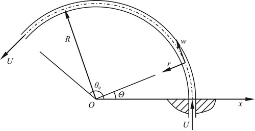
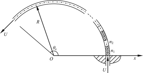
A general cantilevered curved pipe conveying fluid is plotted in Figure 1, where w and r separately denote tangential and radial displacement of a random point on the centerline, R is the constant radius of the centerline, Θ is the angle coordinate and θ_c is the opening angle of the pipe.

Figure 1. Mechanical model of cantilevered curved pipe conveying fluid.

As reported by Misra et al. (1988a, 1988b), the conclusions based on the modified inextensible and extensible theories for curved pipes with both ends supported regarding stability are more reliable, mainly due to the contribution of steady combined force (also named ‘initial axial force’), while for cantilevered one, effect of this force seems less pronounced and hence can be neglected (Wang et al., 2007; Misra et al., 1988a). Therefore, the general linear governing equation (Wang & Ni, 2008) for the centerline of the curved pipe conveying fluid is (1) where

where, m_f and m_p denote the mass per unit length of fluid and pipe, respectively, inner fluid flows with constant velocity U modeled by plug flow, EI represents the flexural stiffness, t is the time, m_t and c_t are the added mass per unit length and the coefficient of viscous damping due to the surrounding fluid, associated with the transverse motion; with m_a and c_a playing similar roles in the longitudinal motion, represents the steady combined force and it equals to zero for the cantilevered curved pipe while for those with both ends supported.

2.2. Application of the new transfer matrix method on the present problem

The solution of Equation (1) can be written as (2) where is a dimensionless natural frequency and Ω corresponds to its dimensional form.

If a cantilevered pipe is considered, with the substitution of Equation (2) into (1) and the representation of with 0, it will become (3)

By means of the Laplace transform and after elementary transformation, the result is (4) where s is the transformed variable in the complex domain, represents the (i–1)th derivative of y(0) and

The denominator in Equation (4) can be factorized as (5)

By means of inverse Laplace transform (Li, Zhao, & Li, 2014), the result will be (6) where, and represents the result substituting s with s_r into .

Then the nth (n = 0, 1, 2, 3, 4, 5) derivative of is (7)

Equation (7) can be reformatted compactly as (8) where, and

According to Equation (2), tangential displacement at the random angle can be expressed as (9)

If the centerline is assumed to be inextensible, the radial displacement, angle of rotation, bending moment, transverse shear force, and axial force can be formulized as (10) (11) (12) (13) (14)

Then the state vector at is (15) where , non-zero terms in is only , likewise, in H they are

Therefore, (16)

It is obvious that Equations (1)–(16) are suitable for the whole pipe, for those pipes possessing inhomogenous factors (including material property, radius of the centerline, geometrical shapes, etc.), the above relationships can be seen as true in each part if the pipe is divided into many short enough elements.

Imagine that for the kth element, numbers of its two boundaries are denoted by k and k + 1, and their angle coordinates are θ_k and θ_k+1, respectively, according to Equations (8), (16), and (15), the following equations can be obtained, i.e. (17) (18) (19)

It is noteworthy that in Equations (17), (18), and (19), subscripts of θ and q denote numbers of node, while those of other variables denote numbers of element. With the substitution of Equation (18) into (17) and then introducing the result into (19), for the kth element, the result can be formulized as (20) where , , l and r denote left and right directions, respectively.

If there exist elastic supports at kth node, then (21) where K and K_t separately denote elastic coefficients in translational and rotational directions.

According to Equation (21), for kth node, the following equation can be obtained, i.e. (22) where, the subscript of F denotes the number of node, and F_ii=1 (i = 1, 2, 3, 4, 5, 6), F₄₃=K_t, F₅₂=-K, and other values equal to zero. Obviously, F will be a unit matrix with six orders if there are no elastic supports.

With the substitution of Equation (22) into (20), it will become (23)

With the combination of Equations (22) and (23), for the nth node, the final expression is (24)

Compactly, Equation (24) can be written as (25)

For the cantilevered pipe, the state vectors at its two ends are (26) (27)

After the combination of Equations (25)–(27), the result is (28)

Let the determinate of the coefficient matrix in Equation (28) equal to zero will surely obtain the dimensionless natural frequency. If and changes its sign at some critical velocity, the pipe will lose stability by divergence (u_cd is used to denote this critical value hereafter), while, If and changes its sign, the pipe will lose stability characterized by flutter (u_cf is used to denote this critical value hereafter).

3. Numerical results

3.1. Verification of the proposed method

By reference to Figure 1, if two spring supports are both implemented on the left end and both elastic coefficients are large enough (e.g. K = K_t=10⁸) so that this end can be seen as completely constrained, then the supporting type will be clamped–clamped, while if K_t=0 and K is large enough, then the problem will transform to a clamped–pinned pipe.

If , β=0.5, K = K_t=10⁸ and the steady combined force is neglected, the critical velocity obtained separately by the proposed method and Huang et al. (2002) are shown in Table 1.

Table 1. Critical velocity by two methods.

Mode	Proposed method	Result of Huang et al.
1st	3.8389	3.8414
3rd	5.4301	5.4318

As Table 1 shows, the results obtained by these two methods agree well with each other, which reveals the validity of the proposed method in calculating the critical velocity.

3.2. Examples

Three examples are introduced in this subsection, i.e. cantilevered, elastically supported, and periodic cantilevered curved pipes conveying fluid, respectively. The focus is not only to study the dynamics of each model but also to show the broad applications of the proposed method.

3.2.1. Cantilevered curved pipe conveying fluid

A pure cantilevered curved pipe has been plotted in Figure 1, and physical parameters of this piping system can be referred in Table 2.

Table 2. Physical parameters of the piping system.

Pipe						Fluid
R (m)	Inner radius r1 (m)	Outer radius r2 (m)	Density ρs (kg/m^3)	Elastic modulus E (GPa)	Opening angle θc (rad)	Density ρf (kg/m^3)
1	0.012	0.014	7800	210	π	1000

According to Table 2, flexural stiffness EI and mass ratio β can be calculated, separately they are EI = 182.252 N m² and β=0.262. ‘Pure’ hereby means there are no inhomogeneity and extra supports, it is a homogeneous cantilevered pipe and hence there is no need dividing the pipe. If , then with the aid of the proposed method, Figure 2 shows the former four orders natural frequency as a function of the flowing velocity in the dimensionless domain.

Figure 2. Real and imaginary parts of natural frequency versus flowing velocity. (a) Real part of natural frequency. (b) Imaginary part of natural frequency.

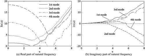
According to Figure 2, all modes decline at first, in addition, the 2nd and 4th modes lose stability via flutter type at u_cf=3.140 and 5.714, respectively, as for other two modes, there are no instabilities over the computing range.

As mentioned in Section 3.1, change of elastic coefficients of springs at left end will lead to distinct supporting types, it will be an interesting issue if the steady combined force is neglected when clamped–clamped and clamped–pinned curved pipes are studied, and Figure 3 shows the results.

Figure 3. Real part of natural frequency of clamped–clamped and clamped–pinned curved pipes versus flowing velocity with (a) Clamped–clamped curved pipe (b) Clamped–pinned curved pipe.

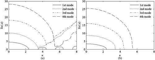
All calculated modes decline sharply if and there exist chances for the pipe to lose stabilities, e.g. for the clamped–clamped curved pipe, it diverges at u_cf=2.360 at its 1st mode, which is certainly not a reliable conclusion compared with Misra’s analysis (1988b). For the clamped–pinned pipe, all four modes decrease following the increase of the flowing velocity at first as Figure 3(b) shows and converge to be a single value after u = 5.5, which is also an unreliable conclusion.

3.2.2. Elastically supported curved pipe conveying fluid

To improve the system’s stiffness, elastic supports are often introduced to support the pipe in practice, and hence this model will be studied in this subsection. It is obvious whether the springs are implemented on the free end or not will lead to dramatically different results. Figure 4 shows the mechanical models corresponding to these two cases.

Figure 4. Mechanical models of cantilevered curved pipe conveying fluid with end-implemented and intermediate elastic supports. (a) Cantilevered curved pipe with end-implemented elastic supports. (b) Cantilevered curved pipe with intermediate elastic supports.

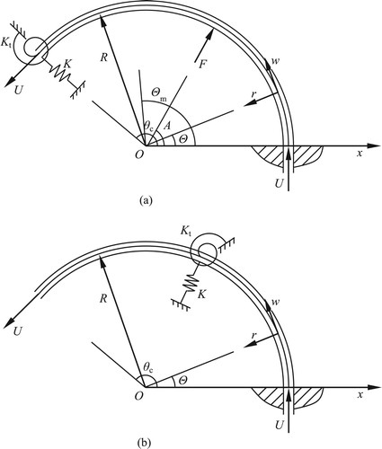
Figure 5 shows the dimensionless natural frequency as a function of the elastic coefficients K and K_t (Both of them are dimensional variables with units in N/m and N m/rad, respectively, for convenience, their units are omitted hereafter.), where the mechanical model corresponds to Figure 4(a) and other parameters are same with Table 1.

Figure 5. Natural frequency versus flowing velocity and elastic coefficients. (a) K = K_t=10, (b) K = K_t=10², (c) K = K_t=10³, (d) K = K_t=10⁴.

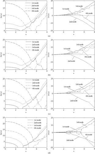
Figure 5 shows that the change of the elastic coefficients will lead to different instabilities, e.g. when K = K_t=10, the 2nd and 4th modes lose stability by flutter at u_cf=3.155 and 5.720, respectively. While in Figure 5(b) (i.e. K = K_t=10²), only the 2nd mode flutters at u_cf=3.230. When K and K_t increase to 10³, the 1st mode will diverge at u_cd=2.673 and the divergence interval is [2.673, 3.042], the 2nd mode flutters at u_cf=3.268. However, as Figure 5(d) shows, if K and K_t increase continuously and reach to 10⁴, all calculated four modes occur instabilities via different types, i.e. the 1st and 3rd modes separately start to diverge at u_cd=2.357 and 4.534, meanwhile, the divergence intervals are [2.357, 3.384] and [4.534, 5.354], the 2nd and 4th modes flutter at u_cf=3.300 and 5.379, respectively.

It is noteworthy that during the above calculation, the steady combined force is neglected, i.e. , while in fact, the rotating and moving freedoms at the free end are constrained to some extent due to the elastic supports, only that the degree is not 100% therefore, the inextensible theory of the centerline appears not appropriate hereby, omitting this force will lead to results departing from true values, especially, if elastic coefficients are bigger, the degree of deviation will be larger simultaneously. Strictly speaking, the supports at both ends mentioned in modified inextensible and extensible theories are supposed to be rigid (clamped or pinned), for flexible supports (i.e. elastic supports in this subsection), is no longer a fixed value, but a variable with respect to elastic coefficients. Thereupon, it should be limited in an interval, i.e. , as for how to evaluate the specific value, to the best of authors’ knowledge, there is no relevant literature over the world till today. To manifest the effect of on the results, with the aid of the present method, real parts of former four modes as a function of the flowing velocity and are calculated and plotted as Figure 6 shows, where K = K_t=10³ and other parameters are same with before.

Figure 6. Natural frequency versus flowing velocity and (a) 1st mode (b) 2nd mode (c) 3rd mode (d) 4th mode.

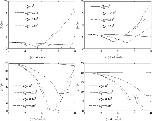
Things will be extremely distinct if takes different values as Figure 6 shows, e.g. for , there’s no instability over the computing range. While for , the 1st mode diverges among [2.689, 3.049], and the 2nd mode flutters at u_cf=3.289. When , the 1st mode diverges among [2.820, 3.205], and the 2nd mode flutters at u_cf=3.503. If , the 1st mode will diverge among [3.781, 4.303], and the 2nd mode will flutter at u_cf=5.222. The results verify that indeed has quite significant influences on the stability of the pipe.

If the springs are implemented intermediately, i.e. the mechanical model as Figure 4(b) shows, things will be different. If inhomogeneity is also neglected, K = K_t, and other parameters are same as Table 1, then two elements are needed in total here. Figure 7 shows u_cf of the 2nd mode as a function of non-dimensional implementation position θ_m and elastic coefficients K and K_t.

Figure 7. u_cf versus θ_m and K, K_t.

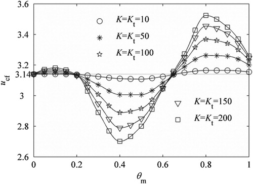
As shown in Figure 7, all curves fluctuate following the increase of θ_m, whatever the elastic coefficients are, and they all start from θ_m=0, u_cf=3.140, mainly in that θ_m=0 means there are no elastic supports, leading to a result same with that of the cantilevered pipe. Furthermore, at a random same position, the larger the elastic coefficients are, the larger u_cf will be obtained, in addition, there are two local peaks and one valley for each curve, all curves reach valley values around θ_m=0.4 and peak ones around θ_m=0.1 and 0.8. In terms of system’s safety, a comparatively larger critical velocity should be a better choice to ensure the pipe can work regularly in a relatively wider velocity range, in this sense, the present method will be of great help in designing elastic supports (including elastic coefficients and their implementation positions), it belongs to an optimization problem, which is of significant sense in engineering practice and deserves a further study.

3.2.3. Periodic cantilevered curved pipe conveying fluid

Due to the existence of manufacturing errors during production practice, there inevitably exists inhomogeneity in the aspect of material properties in curved pipes, hypothetically, the pipe is divided into finite elements, as long as each element is short enough, the inhomogeneity in the individual element can be approximately neglected. To make things simple, every other element is assumed to have same parameters (including Yong’s modulus, moment of initial, density and length etc.), then Figure 8 shows a periodic pipe under this assumption. If N denotes the number of all elements, with N₁ and N₂ denoting that of elements in length n₁ and n₂, respectively, then N = N₁+N₂ is naturally founding, in addition, if N is an even number, N₁=N/2, otherwise, N₁=(N + 1)/2. is introduced to denote length ratio, and obviously, . λ reaching its two boundaries means the pipe thereby is a cantilevered one, under these two circumstances, the critical velocity should be the same value because it’s a dimensionless variable, which is supposed to have nothing to do with dimensional physical parameters and N.

Figure 8. Mechanical model of periodic cantilevered curved pipe conveying fluid.

If flexural rigidity of the main element (i.e. the element in length n₁) is EI₁=150 N m², and that of the element causing inhomogeneity (i.e. the element in length n₂) is EI₂=200 N m², other parameters are: R = 1 m, β=0.25, θ_c=π, then u_cf of the 2nd mode versus N and λ can be calculated by the proposed method as Figure 9 shows.

Figure 9. u_cf versus N and λ (a) (b) .

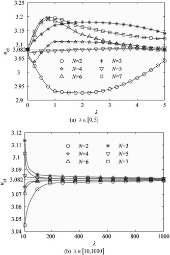
According to Figure 9, it is found that all curves originate from the same point, i.e. λ=0, u_cf=3.082, in addition, with the increase of λ, all curves tend to be gentle, the limiting values converge to 3.082, manifesting that the calculated results anastomose well to the analysis mentioned before, which further verifies the validity of the proposed method. For a specific N, there exist critical length ratios (e.g. λ_c=0.6 for N = 3 and λ_c=2 for N = 5) causing their calculated u_cf to equal to 3.082, which means that appropriate combination of N and λ can be found to approximate a pure cantilevered curved pipe. Meanwhile, when N = 5, its corresponding curve fluctuates in the least range among all calculated curves for random λ, meaning the result now is nearest to a pure cantilevered curved pipe and revealing that there’s nearly no necessity to divide the pipe into more segments.

In conclusion, there are two approaches to obtain roughly the same critical velocity with a cantilevered curved pipe, one is controlling the inhomogeneity as little as possible, the other is N equals to an appropriate value that can be calculated by the proposed method.

4. Discussion

As mentioned in Section 3.2.2, for a pipe conveying fluid with one end clamped and the other elastically supported, the initial axial force should be appropriately considered mainly in that the translational and rotation freedoms are partly constrained, but there is difficulty in how to evaluate the force, the only thing we know is , therefore, large quantity of experiments are needed in this sense and the present method will then be of tremendous help in further calculation.

During the construction of the proposed method, one thing of crucial importance needs be noted is the problem researched should be linear with respect to time and hence can be separated out, for a nonlinear problem (Lee & Chung, 2002), the proposed method can do nothing about it mainly for that Laplace transform is an effective tool only in solving linear problem, and hence can be used in this paper to calculate position-related solution, based on which the transfer matrix will then be easy to be constructed, according to this, the method will be helpful in solving linear dynamic problems in other fields, thereupon, there leave sufficient spaces for researchers to improve the application range of this method in further study.

5. Conclusions

Flow-induced vibration problem of curved pipe conveying fluid is investigated in this paper. With the aid of the Laplace transform, the analytical state vector is formulated, and then its transfer matrix is derived. Three examples including cantilevered, elastically supported, and periodic cantilevered curved pipes conveying fluid are investigated, critical velocity for flutter under these circumstances are calculated by the proposed method.

For the fixed-free curved pipe with elastic supports implemented on the free end, if the elastic coefficients increase to large enough, the instability type will be no longer the only flutter, but divergence may appear. For the periodic pipe, controlling N to equal to an appropriate value is a better choice to approximate a pure cantilevered curved pipe in terms of critical velocity in engineering practice.

The proposed method takes advantage of the Laplace transform in solving linear problem, and combining the three examples, it can be concluded that it is feasible for the proposed method to study more complex problems, e.g. periodic curved pipe with intermediate elastic supports, changeable radius of the centerline or their combinative problems, or above all aspects for straight pipes conveying fluid. In conclusion, the proposed method is suitable for solving linear problems characterized by the chain structure.

Disclosure statement

No potential conflict of interest was reported by the authors.

Additional information

Funding

This work was supported by the National Natural Science Foundation of China [grant number 51775097].

References

- Dai, H. L., Wang, L., Qian, Q., & Gan, J. (2012). Vibration analysis of three-dimensional pipes conveying fluid with consideration of steady combined force by transfer matrix method. Applied Mathematics and Computation, 219, 2453–2464. doi:10.1016/j.amc.2012.08.081.
- Enz, S., & Thomsen, J. J. (2011). Predicting phase shift effects for vibrating fluid-conveying pipes due to coriolis forces and fluid pulsation. Journal of Sound and Vibration, 330, 5096–5113. doi:10.1016/j.jsv.2011.05.022.
- Gao, X. P., Zhang, H., Liu, J. J., Sun, B. W., & Tian, Y. (2018). Numerical investigation of flow in a vertical pipe inlet/outlet with a horizontal anti-vortex plate: Effect of diversion orifices height and divergence angle. Engineering Applications of Computational Fluid Mechanics, 12(1), 182–194. doi:10.1080/19942060.2017.1387608.
- Guo, C. Q., Zhang, C. H., & Paidoussis, M. P. (2010). Modification of equation of motion of fluid- conveying pipe for laminar and turbulent flow profiles. Journal of Fluids and Structures, 26, 793–803. doi:10.1016/j.jfluidstructs.2010.04.005.
- Huang, Y., Zeng, G., & Wei, F. (2002). A new matrix method for solving vibration and stability of curved pipes conveying fluid. Journal of Sound and Vibration, 251(2), 215–225. doi:10.1006/jsvi.2001.3983.
- Isenmann, G., Bellahcen, S., Vazquez, J., Dufresne, M., Joannis, C., & Mose, R. (2016). Stage-discharge relationship for a pipe overflow structure in both free and submerged flow. Engineering Applications of Computational Fluid Mechanics, 10(1), 283–295. doi:10.1080/19942060.2016.1157100.
- Karami, H., & Farid, M. (2015). A new formulation to study in-plane vibration of curved carbon nanotubes conveying viscous fluid. Journal of Vibration and Control, 21, 2360–2371. doi:10.1177/1077546313511137.
- Koo, G. H., & Yoo, B. (2000). Dynamic characteristics of KALIMER IHTS hot leg piping system conveying hot liquid sodium. International Journal of Pressure Vessels and Piping, 77, 679–689. doi:10.1016/S0308-0161(00)00057-0.
- Lee, S. I., & Chung, J. (2002). New non-linear modeling for vibration analysis of a straight pipe conveying fluid. Journal of Sound and Vibration, 254(2), 313–325. doi:10.1006/jsvi.2001.4097.
- Li, S. J., Liu, G. M., & Kong, W. T. (2014). Vibration analysis of pipes conveying fluid by transfer matrix method. Nuclear Engineering and Design, 266, 78–88. doi:10.1016/j.nucengdes.2013.10.028.
- Li, Y. D., & Yang, Y. R. (2014). Forced vibration of pipe conveying fluid by the green function method. Archive of Applied Mechanics, 84, 1811–1823. doi:10.1007/s00419-014-0887-1.
- Li, X. Y., Zhao, X., & Li, Y. H. (2014). Green's functions of the forced vibration of Timoshenko beams with damping effect. Journal of Sound and Vibration, 333, 1781–1795. doi:10.1016/j.jsv.2013.11.007.
- Misra, A. K., Paidoussis, M. P., & Van, K. S. (1988a). On the dynamics of curved pipes transporting fluid, part I: Inextensible theory. Journal of Fluids and Structures, 2, 221–244. doi:10.1016/S0889-9746(88)80009-4.
- Misra, A. K., Paidoussis, M. P., & Van, K. S. (1988b). On the dynamics of curved pipes transporting fluid, part II: Extensible theory. Journal of Fluids and Structures, 2, 245–261. doi:10.1016/S0889-9746(88)80010-0.
- Ni, Q., Zhang, Z. L., & Wang, L. (2011). Application of the differential transformation method to vibration analysis of pipes conveying fluid. Applied Mathematics and Computation, 217, 7028–7038. doi:10.1016/j.amc.2011.01.116.
- Paidoussis, M. P. (2008). The canonical problem of the fluid-conveying pipe and radiation of the knowledge gained to other dynamics problems across applied mechanics. Journal of Sound and Vibration, 310, 462–492. doi:10.1016/j.jsv.2007.03.065.
- Wang, L., Liu, H. T., Ni, Q., & Wu, Y. (2013). Flexural vibrations of microscale pipes conveying fluid by considering the size effects of micro-flow and micro-structure. International Journal of Engineering Science, 71, 92–101. doi:10.1016/j.ijengsci.2013.06.006.
- Wang, L., & Ni, Q. (2008). In-plane vibration analyses of curved pipes conveying fluid using the generalized differential quadrature rule. Computers and Structures, 86, 133–139. doi:10.1016/j.compstruc.2007.05.011 doi: 10.1016/j.compstruc.2008.02.007
- Wang, L., Ni, Q., & Huang, Y. Y. (2007). Dynamical behaviors of a fluid-conveying curved pipe subjected to motion constraints and harmonic excitation. Journal of Sound and Vibration, 306, 955–967. doi:10.1016/j.jsv.2007.06.046
- Yu, D. L., Paidoussis, M. P., Shen, H. J., & Wang, L. (2014). Dynamic stability of periodic pipes conveying fluid. Journal of Applied Mechanics, 81(1), 011008. doi:10.1115/1.4024409.
- Zhao, Q. L., & Sun, Z. L. (2017). In-plane forced vibration of curved pipe conveying fluid by Green’s function method. Applied Mathematics and Mechanics (English Edition), 38(10), 1397–1414. doi:10.1007/s10483-017-2246-6.