An ALE formulation for compressible flows based on multi-moment finite volume method

ABSTRACT

A direct Arbitrary Lagrangian Eulerian (ALE) formulation using multi-moment finite volume method for viscous compressible flows on unstructured moving grids has been developed and presented in this paper. High-order polynomials are reconstructed over a compact mesh stencil by making use of both volume integrated average value (VIA) and point values (PV) at the vertices of mesh cells which change in time. By formulating the governing equation in ALE integral form and differential form, the computational variables, VIA and PV, are updated, respectively, by a finite volume scheme and a point-wise discretization using multi-moments (VIA and PV). A simple and efficient formulation is derived for moving mesh which satisfies the geometrical conservation law. In the computations involving moving-body, the PVs of velocity at the vertices of cells adjacent to the body surface are coincided with the motion of the body, which eliminates the numerical approximation to find the cell boundary values on the body surface in conventional finite volume method. Numerical tests are presented to verify the present method as a high-order ALE formulation for compressible flows on both stationary and moving grids.

KEYWORDS:

• Viscous compressible flow
• multi-moment finite volume method
• direct ALE
• moving grids
• compact stencil

1. Introduction

Computational fluid dynamics (CFD) has become an important auxiliary tool for engineering applications (Akbarian et al., 2018; Ardabili et al., 2018; Mou, He, Zhao, & Chau, 2017) in the past several decades. Fluid structure interaction (FSI), as an ubiquitous phenomena in nature and engineering applications, has been being an active research area in CFD community. In many numerical solvers for FSI problems, the computational domain moves or undergoes deformations due to the movement of the domain boundary. Thus, numerical methods on moving grids are desired to maintain accuracy and conservation of the numerical solutions for FSI applications which usually result in more complex flow structures.

There are two classical kinematic descriptions in the simulations of compressible fluid dynamics: i.e. the Lagrangian description and the Eulerian description. Lagrangian algorithms inherently have superiority in tracking free surfaces and interfaces between different materials since the computational cells move with local fluid velocity. However, they may encounter difficulties when the mesh cell tangles due to large flow distortions. Eulerian algorithms are more robust for flow simulations as the computational grids keep stationary during whole computational process. However, it is difficult in some cases to maintain adequate solution quality on fixed computational mesh. Furthermore, in simulations involving interactions of multi-materials, extra numerical procedures are required to identify the interface between different materials, which might generate numerical errors. Due to the shortcomings of purely Lagrangian and purely Eulerian descriptions, Arbitrary Lagrangian Eulerian (ALE) description is firstly proposed in Hirt, Amsden, and Cook (1974) to solve fluid dynamics in a suitably moving and deforming grid. In ALE formulations, the grids for the computational domain can move arbitrarily and independently of the fluid motions, which makes it more robust in moving boundary simulations. ALE methods have been studied for several decades to handle the difficulties in the simulation of multi-material fluid flows with large distortions (Ahn & Kallinderis, 2006; Bazilevs, Takizawa, & Tezduyar, 2013; Donea, Giuliani, & Halleux, 1982; Donea, Huerta, Ponthot & Rodríguez-Ferran, 2004; Duarte, Gormaz, & Natesan, 2004; Liu, 1988; Lhner, 2008). They can be classified into two classes, i.e. indirect method and direct method. The indirect method generally consists of three steps: (1) a Lagrangian step for updating the grid and the solution; (2) a rezoning step to regularize the heavily distorted or tangled mesh cells; (3) a remapping step transferring the Lagrangian solution to the rezoned mesh which is adjusted in step (2). However, it may be computationally expensive especially for three dimensional realistic calculations due to rezoning and remapping steps. The direct ALE method (Boscheri, Loubére, & Dumbser, 2015; Persson, Bonet, & Peraire, 2009) includes the grid velocity in the numerical formulation, which is consistent with the moving mesh framework. Thus, the remapping procedure is not needed as a separate step. Both direct and indirect methods are widely implemented in CFD.

To construct high-order ALE scheme, existing works of indirect ALE scheme start from the purely Lagrangian framework. Cheng and Shu (2007) proposed a class of Lagrangian type schemes based on high-order essentially non-oscillatory (ENO) reconstruction (Harten, Engquist, Osher, & Chakravarthy, 1987) and obtained third-order accuracy for Euler equations with curved mesh in Cheng and Shu (2008). Dumbser, Uuriintsetseg, and Zanotti (2013) developed a one-dimensional high-order Lagrangian arbitrary high-order accurate (ADER) finite volume method. The discontinuous Galerkin (DG) method has also been implemented in the Lagrangian formulation for solving gas dynamic equations (Vilar, Maire, & Abgrall, 2014). The purely Lagrangian framework shows the strong ability for capturing the contact discontinuities since no advection term is included in the formulation. However, the subsequent rezoning and remapping steps are always needed to adjust the heavily distorted meshes for large distortion problems. For high-order direct ALE schemes, Clair et al. added an edge-based upwind numerical fluxes of ALE part to a conventional cell-centered Lagrangian solver as presented in Clair, Ghidaglia, and Perlat (2016). Boscheri et al. developed high-order direct ALE ADER finite volume formulations in Boscheri and Dumbser (2014) and Boscheri et al. (2015) with weighted essentially non-oscillatory (WENO) reconstruction and multi-dimensional optimal order detection (MOOD) approach.

Moreover, high-order discontinuous Galerkin (DG) direct ALE methods have been implemented in Lomtev, Kirby, and Karniadakis (1999), van der Vegt and Van der Ven (2002), Nguyen (2010), Persson et al. (2009), Mavriplis and Nastase (2011), and Ren, Xu, and Shyy (2016). In the present research, we are interested in constructing a high order and more efficient direct ALE method for compressible Navier–Stokes equations.

As stated above, there are mainly two methodologies to devise high-order ALE schemes. One is based on the conventional finite volume method, which uses wide stencils to generate high-order polynomials. However, choosing the reliable cell stencils on moving grids is not an easy task for distorted or unstructured grids which are commonly used in applications. The other methodology is to use compact stencils by adding the degrees of freedoms (DOF) locally on each cell, such as the DG method (Cockburn, Lin, & Shu, 1989; Cockburn & Shu, 1989) and the spectral finite volume method (Wang, 2002; Wang & Liu, 2002). Such methods have superior properties for achieving high-order accuracy. On the other hand, for moving boundary problems, especially for fluid-structure interaction applications, the solutions, as well as the coupling conditions, on the fluid-structure interfaces are crucial and require particular attention. Since the aforementioned methods based on increased local DOFs define the computational variables inside each cell, extra numerical steps are needed to determine the values and conditions on the body surfaces or interfaces among different materials.

It is sensible to use the PVs at cell vertices located on the material surfaces as computational variables which are updated at every time step. With these PVs known on the surfaces, the interactions among different materials can be handled in a more accurate and convenient manner. This observation motivates us to re-cast the ALE formulation using both volume integrated average (VIA) and point values (PV) at the cell vertices as the computational variables, i.e. the underlying idea of the multi-moment finite volume method. Multi-moment finite volume method based on local reconstruction was developed by Xie, Ii, Ikebata, and Xiao (2014) and Xie and Xiao (2014) on unstructured grids to achieve high-order accuracy for incompressible flows in Eulerian representation with fixed grids. In multi-moment finite volume method, both VIA and PVs are used for local polynomial reconstruction, and simultaneously they are treated as computational variables which are solved by integral form and differential form of the governing equations, respectively. Successive works for Euler equations have been implemented in Xie, Deng, Sun, and Xiao (2017) and Deng, Xie, and Xiao (2017). Since the high-order polynomial is based on well-determined local cells, it is straightforward to extend previous studies to moving grids. This research focuses on constructing a 2D multi-moment finite volume ALE scheme for viscous compressible flows on moving grids.

We formulate the governing equations in ALE integral form and ALE differential form to update the VIAs and PVs, respectively. The 2D computational domain is partitioned with triangular mesh elements, which facilitates implementations for complex geometries. The computational variables, the VIAs and the PVs at the moving cell vertices, are used to build the local high-order reconstruction consistent with moving mesh, which is similar to the Eulerian framework. The integral form is discretized by the conventional finite volume scheme, where the convective fluxes for VIA can be calculated by commonly used Riemann solvers, such as Rusanov scheme (1962), HLL scheme (Harten, Lax, & van Leer, 1983) and HLLC scheme (Toro, 2013), while the gradients of physical variables on the edge for viscous terms are simply interpolated from the neighboring cell centers. The differential form is discretized by the finite difference scheme in which Roe's Riemann solver (1981) is used for the inviscid flux and the viscous flux term is calculated by (Time-evolution Converting) formulation as shown in Xiao, Akoh, and Ii (2006). The geometrical conservation law (GCL) is automatically satisfied in the present ALE formulation where the mesh cells are moved with the specified velocities at the mesh nodes while the edges of the moving mesh cells remain as straight-line in 2D or planar in 3D. Though linear grid velocity distribution is assumed on cell edge, it does not degrade the accuracy (convergence rate) of the ALE framework as shown later in the numerical tests.

To verify the proposed scheme for moving grids, three kinds of mesh movement strategies are used in this research: (1) mesh moves with the local fluid velocity; (2) mesh moves following an analytical function; (3) mesh moves by RBF (radial basis function) interpolation (Bos, 2010; De Boer, Van der Schoot, & Hester, 2007; Estruch & et, 2013) for moving boundary problems.

The rest of this paper is organized as follows. Section 2 gives the ALE integral form and differential form of the governing equations. Section 3 presents the multi-moment reconstruction formulation for triangular elements. The numerical formulation for viscous compressible flow is presented in Section 4. In Section 5, numerical tests are given for verifications. We close the paper in Section 6 by some conclusion remarks.

2. Governing equations

2D compressible Navier–Stoke equations in Eulerian coordinates can be formulated in the system of conservation laws (1) where represents the vector of conservative variables, and represent the vectors of convective flux and viscous flux, respectively. In this formulation, the vector of conservative variables and fluxes take the form as follows (2) with and E being the density, velocity, pressure, momentum and specific total energy of the fluid, respectively. The symbol ⊗ denotes the tensor product and is the unit tensor. Based on Stoke's hypothesis, the stress tensor is a linear function of velocity gradient given as (3) The dynamic viscosity μ is represented as a function of temperature T following Sutherland's law (4) The heat flux vector is given by (5) where is the thermal conductivity with Pr and being Prandtl number and the specific heat capacity at constant pressure, respectively. We also include the equation of state to establish the relationship among three thermodynamic variables in the following general form (6) where is the specific internal energy. We consider the ideal gas in the research with the simpler form as . The adiabatic index is the ratio of specific heat capacities at constant pressure and constant volume conditions and we set in this research unless otherwise stated.

2.1. Integral form

Following Mavriplis and Yang (2006), we integrate Equation (1(1) ) over a moving control volume which is enclosed by its boundary as (7) where denotes the surface normal vector of the control volume boundary . Using the differential identity (8) Equation (7(7) ) becomes (9) In this research, we denote the vector of convective flux and viscous flux as and , respectively, with representing the grid moving velocity. Thus, we formulate the ALE integral form of compressible Navier–Stoke equations as (10) In the case of uniform flow, where all fluid variables are uniform and constant, Equation (10(10) ) should be reduced to (11) which is the original definition of GCL (Thomas, 1979) in the integral form. Here, V is the control volume.

2.2. Differential form

With the relation between spatial time derivatives and referential time derivatives, Equation (1(1) ) can be written as (12) where denotes the time derivative of conservative variables with respect to grid moving frame. Equation (12(12) ) can also be cast in the standard quasi-linear form in 2D as (13) where and are the Eulerian Jacobian matrices, is the unit matrix, and are x and y components of grid velocity , respectively. Thus, we formulate the ALE differential form of compressible Navier–Stoke equations as (14) with the ALE Jacobian matrices and . Here, and are the diagonal matrices of original Eulerian Jacobian matrices and . and are the right and left eigen matrices of the corresponding matrices (). We also denote , with , , , , , for simplicity.

Since the grid velocity is considered in both integral and differential formulations, the system can be discretized on arbitrarily moving grids. Two common cases are: (1) Eulerian framework with in which mesh keeps stationary; (2) Lagrangian framework with where the control volume moves with the local fluid velocity.

3. Multi-moment reconstruction formulation

3.1. The grid configuration and notations

In this study, we partition 2D computational domain into non-overlapping straight-line triangular elements, denoted by , . Therefore, it is simple to generate computational meshes for arbitrary geometries. And we denote the global nodes (vertices of element cells) by , . The surrounding cells sharing node are denoted by ().

To reconstruct the high-order polynomials on local cells, we further denote the three vertices of cell by with the coordinate , and its three boundary line segments by , and as shown in Figure 1(a). The length and outward unit normal vector of segment , are and , respectively. The element area and mass center of are and , respectively.

Figure 1. (a) Triangular element, (b) Definition of moments (computational variables).

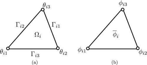
Two kinds of computational variables, i.e. the VIA over and the PV at the vertices of cell are defined as (15) (16) as shown in Figure 1(b), where φ stands for the conservative variables .

3.2. Local reconstruction

Following Xie et al. (2014) and Xie and Xiao (2014, 2016), the triangular cell on physical coordinates is transformed to a reference element in local coordinate with the transformation (17) where . We first calculate the first-order derivative of the physical field at cell center in the physical coordinates by using least square method and then transform it into the local coordinates as . With the supplementary of , the reconstruction polynomial can be formulated on the local coordinates as (18) where the coefficients can be determined by the following constraints (19) With above formulations, the first-order derivatives at vertices are firstly computed from the reconstruction functions in local coordinates and then transformed back to the physical coordinates as .

3.3. Spatial derivatives

With the spatial derivatives of physical field at global node , , calculated from the surrounding cells , the upwind-biased derivatives at point are approximated by (20) The weights here are calculated by (21) where denotes the vector from the mass center to vertex , and the unit normal vector represents and , respectively.

4. Numerical formulation

4.1. Solutions of Navier–Stokes equations for VIA moment

We formulate the semi-discrete form for Equation (10(10) ) with a Q-point Gaussian quadrature for surface convective fluxes and a relatively simpler integration for viscous fluxes as (22) where denotes the VIA of conservative variables on cell with volume , is the Gaussian quadrature point on cell edge which separates cells and . Two-points Gaussian quadrature formula is used in this work, which reads and for the edge with endpoints and .

Various Riemann solvers for calculating the inviscid flux on edge are implemented in this research, such as the robust Rusanov scheme (1962), HLL scheme (Harten et al., 1983) and the less diffusive HLLC scheme (Luo, Baum, & Löhner, 2004). HLLC scheme is mainly adopted in this research. Rusanov and HLL schemes are employed to problems involving strong shock waves to stabilize the computation.

The viscous numerical fluxes are evaluated based on the values and of conservative variables on cell edge segment . Thus, we formulate the viscous flux on the edge as (23) where and are reconstructed line-averaged values of two neighboring cells, respectively, is linearly interpolated from the spatial derivatives in the cell center of the two neighboring cells.

4.2. Solutions of Navier–Stokes equations for PV moment

We solve Equation (14(14) ) point-wisely by Roe's Riemann solver (1981) for convective term and (Time-evolution Converting) formulation (Xiao et al., 2006) for viscous term as (24) where the matrices with tilde are calculated from the Roe-averaging values of the surrounding VIAs as (25) and the sound speed is approximated by (26)

4.3. Geometrical conservation law

For a uniform flow, the spatial gradients of all flow variables are zero, thus Equation (22(22) ) becomes (27) which is the semi-discretization of GCL. Here, is the grid velocity at Gaussian point on edge . For an arbitrarily varying mesh, we can suppose that the grid velocity has a linear distribution over cell edges. Given the grid velocities at two ends of boundary segments denoted as and , Equation (27(27) ) can be simplified as (28) where the edge-averaged velocity is given as (29) It is noted that, by the assumption that the cell edge moves as a solid body, Equation (28(28) ) might not truly realize the pure Lagrangian framework for deformational flows because the cell boundaries do not move with the local fluid in the same accuracy order of the third-order spatial discretizations. As shown in Cheng and Shu (2008), curvilinear meshes are necessary for purely Lagrangian scheme higher than second order. Nevertheless, by assuming cell boundaries always move as a linear edge and then computing the numerical fluxes over this linear edge, it is still possible to achieve third-order accuracy for the ALE framework. We call the framework that only moves cell vertices with the local fluid as quasi-Lagrangian framework in this research to distinguish it from the purely Lagrangian framework.

5. Numerical results

Third-order Runge–Kutta scheme is used for time integration. Since the mesh geometry changes in time, not only VIAs and PVs but also the geometrical quantities, such as volumes, boundary surfaces and vertices of moving cells are updated at each Runge–Kutta sub-step in the simulation.

5.1. 2D isentropic vortex

To examine the convergence rate of inviscid part of the present scheme, the propagation of an isentropic vortex (Shu, 1998) benchmark test is calculated. we compute this problem on an initial computational domain and specify the initial conditions in terms of primitive variables as (30) where are the initial vortex perturbations. We set this perturbation at the center of computation domain with the vortex strength . Then the initial perturbations are given as following, (31) where denotes the temperature perturbation, and . The initial profile of density is presented in Figure 2 (a).

Figure 2. (a) Initial profile of 2D isentropic vortex; (b) and (c) show the density results with the present scheme in Eulerian framework and quasi-Lagrangian framework at time t=1. (a) Initial condition, (b) Eulerian and (c) quasi-Lagrangian.

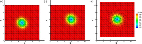
We compute this problem to time t=1 in the Eulerian and quasi-Lagrangian framework respectively with gradually increased number of triangular elements. The periodic boundary condition is applied. The final vortices of density calculated on 800 triangular elements show in Figure 2. To verify that the mesh can move arbitrarily for the proposed scheme, we also calculate the same case on a specific moving mesh framework where the mesh moves independent of fluid motion. 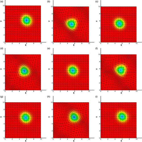The grid velocities vary with time as (32a) (32b) where Figure 3 shows the density and mesh variation with time. Though the mesh moves independent of fluid motion, the vortex propagates in the domain and accurately reproduced during whole computation process.

Figure 3. Density and grid variation for vortex advection with the grid velocity given in Equation (32(32a) ).

For this advection test of isentropic vortex, the analytical solution is available, which is just the time-shifted initial profile for the distance of 1 in both x and y directions. Thus we measure the and errors of the Eulerian, quasi-Lagrangian and the specific-speed moving frameworks, and show the results in Table 1. As expected, third-order numerical accuracy is achieved for all of these three frameworks. It also demonstrates that higher than second-order accuracy can be achieved for linear edge element by ALE scheme.

Table 1. Errors and convergence rates of density for 2D isentropic vortex.

	Eulerian				Quasi-Lagrangian				Specific-speed ALE
cells		rate		rate		rate		rate		rate		rate
200	4.16e–3	−	7.10e–2	−	3.12e–3	−	5.15e–2	−	5.78e–3	−	1.06e–1	−
800	8.01e–4	2.38	1.76e–2	2.01	6.06e–4	2.36	9.70e–3	2.41	1.46e–3	1.99	3.04e–2	1.81
3200	1.16e–4	2.78	3.07e–3	2.52	7.94e–5	2.93	1.35e–3	2.85	2.42e–4	2.59	5.12e–3	2.57
12,800	1.47e–5	2.99	3.87e–4	2.99	9.50e–6	3.06	1.52e–4	3.15	3.18e–5	2.92	6.59e–4	2.96
51,200	1.85e–6	2.99	4.81e–5	3.01	1.15e–6	3.04	1.75e–5	3.12	4.03e–6	2.98	8.24e–5	3.00

5.2. Free stream preservation

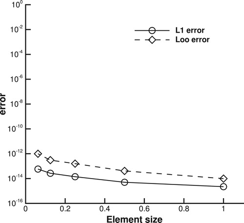
Free stream preservation is a common test to check the GCL for moving mesh schemes. The computational domain and mesh are set as the same as in Section 5.1. The initial conditions are uniform for all physical fields with . We compute this test up to time t=1 with mesh moving following the formulations (32a(32a) ) and (32b(32b) ), and plot the and numerical errors of density for meshes with different element sizes as shown in Figure 4. The numerical errors for all mesh resolutions are of machine precision, which justifies the exact geometrical conservation of the proposed method.

Figure 4. and errors of density for meshes with different element sizes.

5.3. Saltzman problem

Saltzman problem is a well-known challenging benchmark test to assess the robustness of numerical algorithms involving mesh movement, which consists of a strong piston-driven shock wave as shown in Boscheri and Dumbser (2013), Maire (2009), Maire, Loubére, and Vchal (2011), and Boscheri, Dumbser, and Zanotti (2015). It is firstly proposed by Dukowicz and Meltz (1992) for a two-dimensional uniformly skewed Cartesian grid in a computational domain of which is discretized by quadrilateral elements. The skewed coordinate of grid is transformed from the uniform Cartesian grid by (33) In this research, each quadrilateral element is split into two triangular elements as shown in Figure 5. The initial condition is given by an ideal gas () with . The gas is pushed by a moving piston from left to right with velocity . A moving slip wall boundary condition is set for the piston on the left and reflective boundary condition is set for other boundaries. The analytical solution is a one-dimensional infinite strength shock wave that moves toward right direction at speed with a post-shock density plateau of 4. 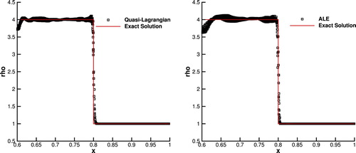To meet the motion of the left piston, we performed the simulation to time t=0.6 in a quasi-Lagrangian framework and also in a specific-speed ALE framework where the mesh movement is given as (34) We use Rusanov scheme (1962) for convection flux and multi-dimensional limiting process (MLP) scheme (Park, Yoon, & Kim, 2010; Xie et al., 2017) is employed for suppressing numerical oscillations. The mesh and density map at final time are given in Figure 6 for both frameworks and density values for the whole field are plotted in Figure 7. Since the ideal gas is filled in the closed container, we also measure the total mass of the gas. The mass variation with time is of machine error, which verifies the conservation of the present scheme.

Figure 5. Initial mesh configuration of Saltzman problem.

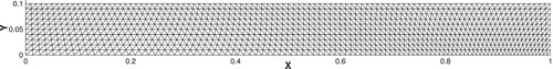
Figure 6. Mesh and density map for Saltaman problems at time t=0.6. (a) The quasi-Lagrangian framework (b) an ALE framework with a specific mesh moving strategy as given in Equation (34(34) ).

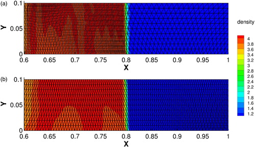
Figure 7. Density values in all cells for Saltzman problem at time t=0.6. (a) The quasi-Lagrangian framework (b) an ALE framework with a specific mesh moving strategy as given in Equation (34(34) ).

5.4. Viscous double Mach reflection

Double Mach reflection is originally proposed by Woodward and Colella (1984) for compressible Euler equations, which involves a Mach 10 shock that hits a ramp. We run a viscous version of double Mach reflection (Dumbser, Peshkov, Romenski, & Zanotti, 2016) in this section to verify the capability of the present solver for simulating viscous flows. The computational domain is set as . The initial conditions, which can be obtained by Rankine–Hugoniot conditions, are given here as (35) Reflecting wall lies along the bottom of the domain where . Analytical solution of a shock Mach number is imposed on the upper wall and bottom wall (). Inflow and outflow boundary conditions are set for left and right sides, respectively. We partitioned the domain into totally 296,418 triangular elements with 640 and 200 uniform segments in the corresponding boundaries. Constant dynamic viscosity is used in this calculation. The other parameters are: , , with .

We first performed the inviscid case up to time t=0.2 with HLL Riemann solver (Harten et al., 1983) for inviscid finite volume flux, and also MLP scheme (Park et al., 2010; Xie et al., 2017) is used for limiting process. The well resolved vortex structures as shown in Figure 8 demonstrate the high fidelity of present method. For viscous shock waves, the Reynolds number is defined based on the shock speed and an unitary reference Length (L=1) as with . We then calculate the cases with and and the comparisons with inviscid case are shown in Figure 9. We observe that, with a rather larger physical viscosity, the small-scale vortex structures are suppressed, which is comparable with Dumbser et al. (2016).

Figure 8. Numerical results of inviscid double Mach at t=0.2 with 296,418 triangular elements. 31 density isolines in the the interval [1,17].

Figure 9. Comparison of (a) inviscid case (b) and (c) at t=0.2 with 296,418 triangular elements. 31 density isolines in the the interval [1,17]. (a) inviscid, (b) , and (c) .

5.5. Flow over cylinder

Flow around a fixed or oscillating cylinder is a widely used benchmark test to evaluate numerical models for fluid-structure interactions. We firstly compute the flow past a fixed cylinder to test the performance of the present solver for stationary grids, and then simulate the flow past a transversely oscillating cylinder to verify its capability for moving boundary problems.

5.5.1. Fixed cylinder

A fixed cylinder of diameter d=1 is located at the origin and the computational domain is set as a rectangular of . The Reynolds number based on the cylinder diameter is defined as and Mach number based on frees-tream flow is given as , where and are the x-component of inlet velocity and inlet sound speed, respectively. To obtain the desired Reynolds number Re=150 and Mach number , we set initial conditions and the Prandtl number Pr=1. The linear viscosity law is chosen in the calculation with and s=0. To avoid the reflection of shock wave from boundaries, the characteristic boundary condition (Carlson, 2011) is used for inlet and outlet boundary. The slip boundary condition is set for top and bottom walls.

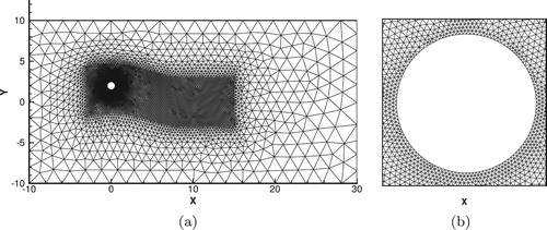
The grid dependency test was firstly conducted to choose a reliable mesh for later simulations. The computational domain is partitioned by a mesh of triangular elements, where the area near the cylinder has relatively smaller cell sizes in order to adequately represent the geometric configuration of the solid body as well as the induced wake and vortex structures. 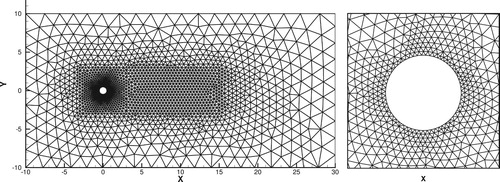Three kinds of grids, Grid A, Grid B and Grid C, are generated where distances between neighboring points on the cylinder are around , and , respectively. Accordingly, the total element numbers for Grid A, Grid B and Grid C are 4358, 14,060 and 48,163, respectively. Figure  10(a) shows the image of Grid A, and the enlarged view of the grid cells near the cylinder is plotted in Figure  10(b).

Figure 10. The mesh image for grid A (a), and the enlarged part near the cylinder surface (b).

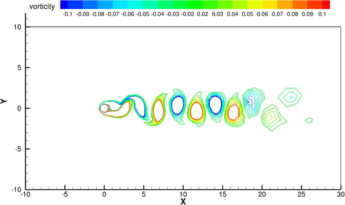
The simulations were performed until final time t=1000 on Grid A, Grid B and Grid C, respectively. We show the numerical results for the case of Re=150 on Grid B in Figure 11 for Mach number and Figure 12 for vorticity. The Krmn vortex street was clearly reproduced after the symmetrical flow structure in the earlier stage was broken.

Figure 11. Mach number distribution for flow over a fixed cylinder at time .

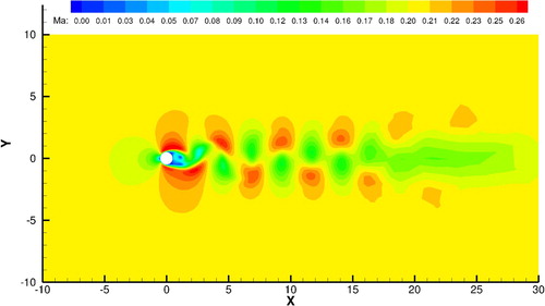
Figure 12. Contours of vorticity for flow over a fixed cylinder at time .

To quantitatively analyze the numerical accuracy, we measure the drag coefficient and the lift coefficient which are calculated as (36) where and are the drag force and the lift force exerted on the cylinder. We plot the drag and lift coefficients for the case calculated on Grid C in Figure 13. In the initial stage of computation, the wake around the cylinder keeps symmetry, thus the lift coefficient approaches zero. With the development of instability, the vortex sheds with gradually increasing shedding amplitude in the downstream of the cylinder and finally the periodic regime established. The profile of lift coefficient looks very close to the representative results in the literature. Due to the periodic vortex shedding, the drag coefficient correspondingly fluctuates as shown in Figure 13. We then calculated the mean drag coefficient (37) with covering several periods of time span sampled during the periodic regime to reduce the statistical error. The Strouhal frequency is also an important parameter for the Krmn streets, which was calculated from the period of lift coefficient in this research. And then the Strouhal number was calculated by (38)

We measured the time-averaged drag coefficient and Strouhal number St for gradually refined meshes, Grid A, Grid B and Grid C as shown in Table 2. The time-averaged drag coefficients approaches 1.371 and the Strouhal number also converges with the mesh finer than Grid B. Therefore, we assume that Grid B can give adequate accuracy for later test cases. Compared with the existing results, the Strouhal number has a good agreement with results calculated by DG/FV method (Zhang et al., 2014) and Mller's simulation (2008).

Figure 13. Temporal variations of drag and lift coefficients for flow over a fixed cylinder at Reynolds number Re=150.

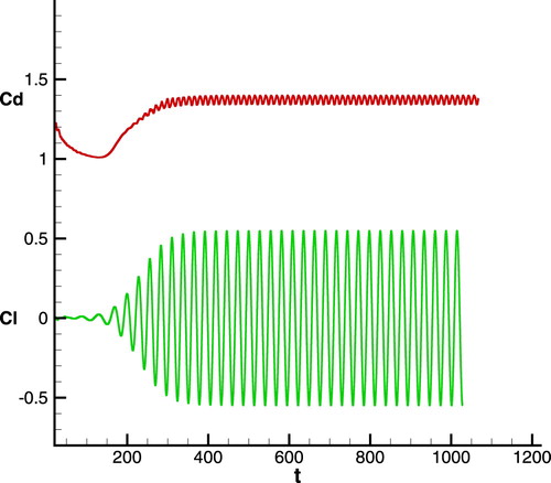
Table 2. Time-averaged drag coefficient and the Strouhal number on gradually refined meshes.

	Time-averaged	Strouhal number St
Grid A	1.364	0.172
Grid B	1.371	0.183
Grid C	1.371	0.184
DG/FV (4th order) (Zhang, Liu, Li, He, & Zhang, 2014)	1.348	0.184
Müller (2008)	1.34	0.183

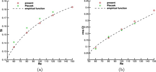
We also calculated the cases with Re=60,80,100 and 120 to evaluate the capability of the numerical model to simulate flows with different Reynolds number. Figure 14 compares the numerical results of Strouhal numbers and r.m.s. (root-mean-square) lift coefficients with the empirical function (Norberg, 2003) and Placzek's numerical results (Placzek, Sigrist, & Hamdouni, 2009). The good agreement of Strouhal number and r.m.s. lift coefficients demonstrates the accuracy of the present solver for stationary mesh, which provides a good base for implementation to moving mesh applications.

Figure 14. Strouhal number and r.m.s. lift coefficient for different Reynolds numbers. (a) Strouhal number and (b) r.m.s. Lift coefficient.

5.5.2. Oscillating cylinder

Viscous flow over oscillating cylinder provides a test bed for numerical solvers for fluid-structure interactions. One of the most interesting phenomena for flow past forced oscillating cylinder is the lock-in phenomenon, which has been reported in the literature to verify numerical models. The characteristics of vortices and wakes around the cylinder is significantly different from that of a fixed cylinder. We investigate the flow over a forced oscillating cylinder in this part with a Reynolds number Re=100.

The cylinder is forced to oscillate in the transversal direction of the main uniform flow with a sinusoidal motion in time defined by (39) where is the maximal displacement which can be characterized by the non-dimensional amplitude . The oscillating frequency, , which associates with the Strouhal frequency for fixed cylinder, plays an essential role in lock-in phenomenon, which can be categorized by the frequency ratio . Figure 15 represents the lock-in zone with respect to the amplitude A and the frequency ratio f where the data is collected from Koopmann and Anagnostopoulos's studies (Anagnostopoulos, 2000; Koopmann, 1967).

Figure 15. Lock-in regime for flow past an oscillating cylinder in (f,A) plane at Re=100 with the data collected from Koopmann and Anagnostopoulos's studies (Anagnostopoulos, 2000; Koopmann, 1967). The region above the data line is the lock-in region and otherwise unlocked region.

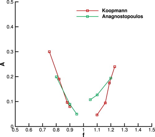
According to Figure 15, we keep the amplitude constant as A=0.3 to devise the locked and unlocked configurations with f=0.5,0.9,1.1 and 1.5. We plot the drag coefficient and lift coefficient over time for four cases in Figure 16 with time characterized by the oscillating period . As expected in Figure 15, the case with f=0.9 and f=1.1 are locked where the vortex shedding frequency are synchronized with the cylinder oscillating frequency as shown in Figure 16(c ,d).

Figure 16. Time variation of drag and lift coefficients for certain frequencies (a)f= 0.5, (b)f=0.9,(c) f=1.1, (d) f=1.5 with A=0.3 at Re=100.

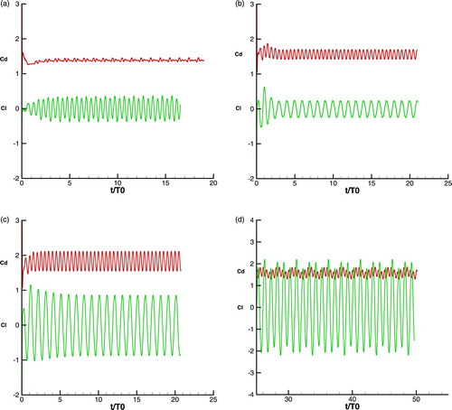
For locked configurations, the mean drag coefficient has a significant increase which reaches 1.56 for f=0.9 and 1.83 for f=1.1, while it is 1.38 for the fixed cylinder. The maximum lift coefficient reduces to 0.24 for f=0.9 but increases to 0.86 for f=1.1, in comparison with its value of 0.33 for the fixed cylinder. Unlocked wakes are formed with the frequency ratio f=0.5 and f=1.5 which represent more complicated phenomena than locked cases. The variation of lift coefficients does not follow the sinusoidal profile any more. The period of signal is over several cylinder oscillation cycles which is called as the beating period . The simpler case is f=0.5 that the beating periodic is equal to the forced oscillation period . In this case, it is twice of the Strouhal period . More complex case is f=1.5 where the beating period consists several oscillating periods as shown in Figure 16(d). The snapshots of vorticity contour lines within one oscillating period are plotted in Figure 17. The cylinder moves with a sinusoidal function in y direction: (a) , it is located at the origin of the domain; (b) , it moves to the maximum displacement in y direction; (c) , it returns to the origin; (d) , it moves to the maximum displacement in the reverse direction of y-axis.

Cases with a larger amplitude A=2 are also calculated to show the ability of our proposed method for large mesh distortions. The oscillating period ratio is set as f=0.5. We show the snapshots of vorticity contour lines within one cylinder oscillating period in Figure 18. Figure 19(a) gives the mesh image when the cylinder moves to the maximum displacement in y direction, and we magnify the area near the cylinder surface in Figure  19(b). By using RBF interpolation function, though large boundary movements are specified, the displacements of the boundary points are smoothly interpolated to the internal grid points based on the distance of the internal nodes to the boundary which is the essence of RBF function to ensure whole mesh maintains a good quality. In the simulation of forced oscillation problems, RBF interpolation is outside the Runge-Kutta loop, which makes the grid velocity constant during the whole time step (including all sub-steps in the 3-stage Runge–Kutta method). It is in fact equivalent to the case that each grid point moves at a constant speed in the duration of each time step. In this way, the computational cost of RBF interpolation can be substantially reduced without losing numerical accuracy. Meanwhile, a coarsening technique is employed as presented in Bos (2010). We select every other five points in the cylinder boundary as control points for saving computational cost. We estimate the computational cost by running the case up to time t=10 on a PC with an Intel Core i7-4790 CPU @ 3.60 GHz, the computational time for RBF interpolation is 48.63 s while the whole running time is 1433.35 s.

Figure 17. The snapshots of vorticity contour lines within one oscillating period . (a) . (b) . (c) . (d) .

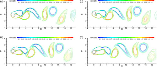
Figure 18. Same as Figure17, but for . (a) . (b) . (c) . (d) .

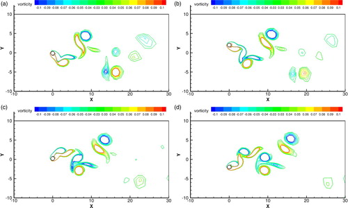
Figure 19. The mesh image for Grid B when the cylinder moves to the maximum displacement in y direction (a), and the enlarged part near the cylinder surface (b).

6. Conclusion remarks

In this paper, we present a multi-moment finite volume method for viscous flows on moving grids based on direct ALE formulation. Two kinds of moments, VIA and PV at cell vertices, are treated as the computational variables and used for constructing quadratic polynomials for moving triangular elements. Both VIA and PV are calculated simultaneously using the integral and differential forms of the governing equations, respectively, under the ALE framework. The VIA is updated by the finite volume method, where conventional Riemann solvers can be used for calculating the convective fluxes and variable gradients on cell edge required in approximating the viscous fluxes are simply calculated from the interpolation of neighboring cell centers. For updating PVs, Roe's Riemann solver is implemented for inviscid fluxes and viscous term is calculated by the (Time-evolution Converting) formula. The GCL is obeyed for deriving the finite volume formulation for control volume variation.

Third-order Runge–Kutta scheme is implemented for not only computational variables but also mesh geometry quantities. Various mesh movement strategies are used for testing the performance of present solver on moving grids: (1) mesh moves with the local fluid velocity; (2) mesh moves following an analytical function; (3) mesh moves by RBF interpolation given boundary points displacements.

Numerical verifications have been carried out in Section 5 to show the performance of the proposed solver. The propagation of 2D isentropic vortex was computed to demonstrate that the present model is able to achieve third-order accuracy on arbitrarily moving triangular elements. The GCL is rigorously satisfied as shown in the free stream preservation test. Compressible flows with high Mach numbers, such as Saltzman problem and viscous double Mach reflection, are calculated to demonstrate the performance of present method. Flow past a cylinder is finally calculated on both stationary and moving grids to show the feasibility for fluid-structure interaction applications. It is pointed out that defining and using the physical variables at the vertices of mesh cells as new computational variables leads to an accurate and efficient numerical formulation for ALE implementation, which can be expected as a novel and promising solver for FSI applications. More applications to multi-material problems, especially strongly coupled FSI problems, are in progress.

Disclosure statement

No potential conflict of interest was reported by the authors.

Additional information

Funding

This work was supported in part by JSPS KAKENHI [grant number 17K18838].

References

- Ahn H. T., & Kallinderis Y. (2006). Strongly coupled flow/struc-ture interactions with a geometrically conservative ALE scheme on general hybrid meshes. Journal of Computational Physics, 219(2), 671–696. doi: 10.1016/j.jcp.2006.04.011
- Akbarian E., Najafi B., Jafari M., Aedabili S. F., Shamshirband S., & Chau K.-w. (2018). Experimental and computational fluid dynamics-based numerical simulation of using natural gas in a dual-fueled diesel engine. Engineering Applications of Computational Fluid Mechanics, 12(1), 517–534. doi: 10.1080/19942060.2018.1472670
- Anagnostopoulos P. (2000). Numerical study of the flow past a cylinder excited transversely to the incident stream. Part 1: Lock-in zone, hydrodynamic forces and wake geometry. Journal of Fluids and Structures, 14(6), 819–851. doi: 10.1006/jfls.2000.0302
- Ardabili S.F., Najafi B., Shamshirband S., Bidgoli B., Deo R. C., & Chau K.-w. (2018). Computational intelligence approach for modeling hydrogen production: A review. Engineering Applications of Computational Fluid Mechanics, 12(1), 438–458. doi: 10.1080/19942060.2018.1452296
- Bazilevs, Y., Takizawa, K., & Tezduyar, T. E. (2013). Computational fluid-structure interaction: Methods and applications. San Diego, CA: John Wiley & Sons.
- Bos F. M. (2010). Numerical simulations of flapping foil and wing aerodynamics: Mesh deformation using radial basis functions (Doctoral dissertation).
- Boscheri W., & Dumbser M. (2014). A direct Arbitrary-Lagrangian Eulerian ADER-WENO finite volume scheme on unstructured tetrahedral meshes for conservative and non-conservative hyperbolic systems in 3D. Journal of Computational Physics, 275, 484–523. doi: 10.1016/j.jcp.2014.06.059
- Boscheri W., & Dumbser M (2013). Arbitrary-Lagrangian-Eulerian one-step WENO finite volume schemes on unstructured triangular meshes. Communications in Computational Physics, 14(5), 1174–1206. doi: 10.4208/cicp.181012.010313a
- Boscheri W., Dumbser M., & Zanotti O. (2015). High order cell-centered Lagrangian-type finite volume schemes with time-accurate local time stepping on unstructured triangular meshes. Journal of Computational Physics, 291, 120–150. doi: 10.1016/j.jcp.2015.02.052
- Boscheri W., Loubére R., & Dumbser M. (2015). Direct Arbitrary-Lagrangian Eulerian ADER-MOOD finite volume schemes for multidimensional hyperbolic conservation laws. Journal of Computational Physics, 292, 56–87. doi: 10.1016/j.jcp.2015.03.015
- Carlson, J. (2011). Inflow/outflow boundary conditions with application to FUN3D. NASA Langley Research Center, Hampton, VA. NASA/TM-2011-217181, L-20011, NF1676L-12459.
- Cheng J., & Shu C.-W. (2008). A third order conservative Lagrangian type scheme on curvilinear meshes for the compressible Euler equations. Communications in Computational Physics, 4, 1008–1024.
- Cheng J., & Shu C.-W. (2007). A high order ENO conservative Lagrangian type scheme for the compressible Euler equations. Journal of Computational Physics, 227(2), 1567–1596. doi: 10.1016/j.jcp.2007.09.017
- Clair G., Ghidaglia J.-M., & Perlat J.-P. (2016). A multi-dimensional finite volume cell-centered direct ALE solver for hydrodynamics. Journal of Computational Physics, 326, 312–333. doi: 10.1016/j.jcp.2016.08.050
- Cockburn B., Lin S.-Y., & Shu C.-W (1989). TVB Runge–Kutta local projection discontinuous Galerkin finite element method for conservation laws III: One-dimensional systems. Journal of Computational Physics, 84(1), 90–113. doi: 10.1016/0021-9991(89)90183-6
- Cockburn B., & Shu C.-W. (1989). TVB Runge–Kutta local projection discontinuous Galerkin finite element method for conservation laws. II. General framework. Mathematics of Computation, 52(186), 411–435.
- De Boer A., Van der Schoot M. S., & Hester Bijl (2007). Mesh deformation based on radial basis function interpolation. Computers & Structures, 85(11–14), 784–795. doi: 10.1016/j.compstruc.2007.01.013
- Deng X., Xie B., & Xiao F. (2017). A finite volume multi-moment method with boundary variation diminishing principle for Euler equation on three-dimensional hybrid unstructured grids. Computers & Fluids, 153, 85–101. doi: 10.1016/j.compfluid.2017.05.007
- Donea J., Giuliani S., & Halleux J.-P. (1982). An arbitrary Lagrangian-Eulerian finite element method for transient dynamic fluid-structure interactions. Computer Methods in Applied Mechanics and Engineering, 33(1–3), 689–723. doi: 10.1016/0045-7825(82)90128-1
- Donea J., Huerta A., Ponthot J.-Ph., & Rodríguez-Ferran A. (2004). Encyclopedia of computational mechanics Vol. 1: Fundamentals. Chapter 14: Arbitrary Lagrangian-Eulerian Methods.
- Duarte F., Gormaz R., & Natesan S (2004). Arbitrary Lagran-gian Eulerian method for NavierStokes equations with moving boundaries. Computer Methods in Applied Mechanics and Engineering, 193(45–47), 4819–4836. doi: 10.1016/j.cma.2004.05.003
- Dukowicz J. K., & Meltz B. JA. (1992). Vorticity errors in multidimensional Lagrangian codes. Journal of Computational Physics, 99(1), 115–134. doi: 10.1016/0021-9991(92)90280-C
- Dumbser M., Peshkov L., Romenski E., & Zanotti Z. (2016). High order ADER schemes for a unified first order hyperbolic formulation of continuum mechanics: Viscous heat-conducting fluids and elastic solids. Journal of Computational Physics, 314, 824–862. doi: 10.1016/j.jcp.2016.02.015
- Dumbser M., Uuriintsetseg A., & Zanotti A. (2013). On arbitrary-Lagrangian-Eulerian one-step WENO schemes for stiff hyperbolic balance laws. Communications in Computational Physics, 14(2), 301–327. doi: 10.4208/cicp.310112.120912a
- Estruch O., Lehmkuhl O., Borrell R., Pérez Segarra C. D., & Oliva A. (2013). A parallel radial basis function interpolation method for unstructured dynamic meshes. Computers and Fluids, 80, 44–54. doi: 10.1016/j.compfluid.2012.06.015
- Harten A., Engquist B., Osher S., & Chakravarthy S. R. (1987). Uniformly high order accurate essentially non-oscillatory schemes, III Upwind and high-resolution schemes (pp. 218–290). Berlin: Springer.
- Harten A., Lax P. D., & van Leer B. (1983). On upstream differencing and Godunov-type schemes for hyperbolic conservation laws. SIAM Review, 25(1), 35–61. doi: 10.1137/1025002
- Herman C., Jiun-Shyan C., & Ted B. (1988). Arbitrary Lagrangian-Eulerian Petrov-Galerkin finite elements for nonlinear continua. Computer Methods in Applied Mechanics and Engineering, 68(3), 259–310. doi: 10.1016/0045-7825(88)90011-4
- Hirt C. W., Amsden A. A., & Cook J. L. (1974). An arbitrary Lagrangian-Eulerian computing method for all flow speeds. Journal of Computational Physics, 14(3), 227–253. doi: 10.1016/0021-9991(74)90051-5
- Koopmann G. H. (1967). The vortex wakes of vibrating cylinders at low Reynolds numbers. Journal of Fluid Mechanics, 28(3), 501–512. doi: 10.1017/S0022112067002253
- Lhner, R. (2008). Applied computational fluid dynamics techniques: An introduction based on finite element methods. Fairfax, Virginia: John Wiley & Sons.
- Lomtev I., Kirby R. M., & Karniadakis G. E. (1999). A discontinuous Galerkin ALE method for compressible viscous flows in moving domains. Journal of Computational Physics, 155(1), 128–159. doi: 10.1006/jcph.1999.6331
- Luo H., Baum J. D., & Löhner R. (2004). On the computation of multi-material flows using ALE formulation. Journal of Computational Physics, 194(1), 304–328. doi: 10.1016/j.jcp.2003.09.026
- Maire P.-H. (2009). A high-order cell-centered Lagrangian scheme for two-dimensional compressible fluid flows on unstructured meshes. Journal of Computational Physics, 228(7), 2391–2425. doi: 10.1016/j.jcp.2008.12.007
- Maire P.-H., Loubére R., & Vchal P. (2011). Staggered Lagrangian discretization based on cell-centered Riemann solver and associated hydrodynamics scheme. Communications in Computational Physics, 10(4), 940–978. doi: 10.4208/cicp.170310.251110a
- Mavriplis D. J., & Nastase C. R. (2011). On the geometric conservation law for high-order discontinuous Galerkin discretizations on dynamically deforming meshes. Journal of Computational Physics, 230(11), 4285–4300. doi: 10.1016/j.jcp.2011.01.022
- Mavriplis D. J., & Yang Z. (2006). Construction of the discrete geometric conservation law for high-order time-accurate simulations on dynamic meshes. Journal of Computational Physics, 213(2), 557–573. doi: 10.1016/j.jcp.2005.08.018
- Mou B., He B.-J., Zhao D.-X., & Chau K.-w. (2017). Numerical simulation of the effects of building dimensional variation on wind pressure distribution. Engineering Applications of Computational Fluid Mechanics, 11(1), 293–309. doi: 10.1080/19942060.2017.1281845
- Müller B. (2008). High order numerical simulation of aeolian tones. Computers & Fluids, 37(4), 450–462. doi: 10.1016/j.compfluid.2007.02.008
- Nguyen V.-T. (2010). An arbitrary Lagrangian–Eulerian discontinuous Galerkin method for simulations of flows over variable geometries. Journal of Fluids and Structures, 26(2), 312–329. doi: 10.1016/j.jfluidstructs.2009.11.002
- Norberg C. (2003). Fluctuating lift on a circular cylinder: Review and new measurements. Journal of Fluids and Structures, 17(1), 57–96. doi: 10.1016/S0889-9746(02)00099-3
- Park J. S., Yoon S.-H., & Kim C. (2010). Multi-dimensional limiting process for hyperbolic conservation laws on unstructured grids. Journal of Computational Physics, 229(3), 788–812. doi: 10.1016/j.jcp.2009.10.011
- Persson P.-O., Bonet J., & Peraire J. (2009). Discontinuous Galerkin solution of the NavierStokes equations on deformable domains. Computer Methods in Applied Mechanics and Engineering, 198(17–20), 1585–1595. doi: 10.1016/j.cma.2009.01.012
- Placzek A., Sigrist J.-F., & Hamdouni A. (2009). Numerical simulation of an oscillating cylinder in a cross-flow at low Reynolds number: Forced and free oscillations. Computers & Fluids, 38(1), 80–100. doi: 10.1016/j.compfluid.2008.01.007
- Ren X. d., Xu K., & Shyy W. (2016). A multi-dimensional high-order DG-ALE method based on gas-kinetic theory with application to oscillating bodies. Journal of Computational Physics, 316, 700–720. doi: 10.1016/j.jcp.2016.04.028
- Roe P. L. (1981). Approximate Riemann solvers, parameter vectors, and difference schemes. Journal of Computational Physics, 43(2), 357–372. doi: 10.1016/0021-9991(81)90128-5
- Rusanov V. V. (1962). Calculation of interaction of non-steady shock waves with obstacles. NRC, Division of Mechanical Engineering.
- Shu C.-W. (1998). Essentially non-oscillatory and weighted essentially non-oscillatory schemes for hyperbolic conservation laws. Advanced numerical approximation of nonlinear hyperbolic equations (pp. 325–432). Berlin: Springer.
- Thomas P. D., & Lombard C. K. (1979). Geometric conservation law and its application to flow computations on moving grids. AIAA Journal, 17(10), 1030–1037. doi: 10.2514/3.61273
- Toro, E. F. (2013). Riemann solvers and numerical methods for fluid dynamics: A practical introduction. Trento: Springer Science & Business Media.
- van der Vegt J. J. W., & Van der Ven H. (2002). Spacetime discontinuous Galerkin finite element method with dynamic grid motion for inviscid compressible flows: I general formulation. Journal of Computational Physics, 182(2), 546–585. doi: 10.1006/jcph.2002.7185
- Vilar F., Maire P.-H., & Abgrall R. (2014). A discontinuous Galerkin discretization for solving the two-dimensional gas dynamics equations written under total Lagrangian formulation on general unstructured grids. Journal of Computational Physics, 276, 188–234. doi: 10.1016/j.jcp.2014.07.030
- Wang Z. J. (2002). Spectral (finite) volume method for conservation laws on unstructured grids basic formulation: Basic formulation. Journal of Computational Physics, 178(1), 210–251. doi: 10.1006/jcph.2002.7041
- Wang Z. J., & Liu Y. (2002). Spectral (finite) volume method for conservation laws on unstructured grids: II Extension to two-dimensional scalar equation. Journal of Computational Physics, 179(2), 665–697. doi: 10.1006/jcph.2002.7082
- Woodward P., & Colella P. (1984). The numerical simulation of two-dimensional fluid flow with strong shocks. Journal of Computational Physics, 54(1), 115–173. doi: 10.1016/0021-9991(84)90142-6
- Xiao F., Akoh R., & Ii S. (2006). Unified formulation for compressible and incompressible flows by using multi-integrated moments II: Multi-dimensional version for compressible and incompressible flows. Journal of Computational Physics, 213(1), 31–56. doi: 10.1016/j.jcp.2005.08.002
- Xie B., Deng X., Sun Z. Y., & Xiao F. (2017). A hybrid pressure-density-based Mach uniform algorithm for 2D Euler equations on unstructured grids by using multi-moment finite volume method. Journal of Computational Physics, 335, 637–663. doi: 10.1016/j.jcp.2017.01.043
- Xie B., Ii S., Ikebata A., & Xiao F. (2014). A multi-moment finite volume method for incompressible Navier Stokes equations on unstructured grids: Volume-average/point-value formulation. Journal of Computational Physics, 277, 138–162. doi: 10.1016/j.jcp.2014.08.011
- Xie B., & Xiao F. (2014). Two and three dimensional multi-moment finite volume solver for incompressible Navier–Stokes equations on unstructured grids with arbitrary quadrilateral and hexahedral elements. Computers & Fluids, 104, 40–54. doi: 10.1016/j.compfluid.2014.08.002
- Xie B., & Xiao F. (2016). A multi-moment constrained finite volume method on arbitrary unstructured grids for incompressible flows. Journal of Computational Physics, 327, 747–778. doi: 10.1016/j.jcp.2016.09.054
- Zhang L. P., Liu W., Li M., He X., & Zhang H. X. (2014). A class of DG/FV hybrid schemes for conservation law IV: 2D viscous flows and implicit algorithm for steady cases. Computers & Fluids, 97, 110–125. doi: 10.1016/j.compfluid.2014.04.002