Research on a method for predicting the underflow concentration of a thickener based on the hybrid model

Abstract

As a method for extracting metals and their compounds, hydrometallurgy has the advantages of high comprehensive metal recovery rate, low environmental pollution, and easier production process. The intensive washing process is a key process in the hydrometallurgical process, and the underflow concentration is a key indicator for measuring the quality of the concentrated washing process. In this paper, after analyzing the characteristics of the thick washing process, the hybrid model combining mechanism modeling and error compensation model based on EDO-TELM (three hidden layers Extreme Learning Machine optimized with Entire Distribution Optimization algorithm) is used to achieve accurate measurement of the underflow concentration in the dense washing process. The hybrid model uses the improved EDO-TELM algorithm as an error compensation model to compensate the error of the un-modeled part of the mechanism model, and gives a reasonable estimate of the uncertain part of the model, which theoretically reduce the prediction error of the model. The Matlab simulation results show that the prediction error of the hybrid model is significantly lower than that of the mechanism model and the data model, and can be adapted to the measurement needs of the industrial site.

KEYWORDS:

• Hydrometallurgy
• underflow concentration
• mechanism model
• EDO
• TELM
• hybrid model

1. Introduction

With the large-scale, centralized and continuous production of hydrometallurgical industry, an efficient and stable automatic production line is urgently required. The overall level of automation of hydrometallurgical production in China is low, and its automation technology greatly restricts the development of hydrometallurgical industry in China (Gui, Yang, Chen, & Wang, 2013). The hydrometallurgical process mainly includes typical processes such as leaching, dense washing, and extraction/replacement (Wang, He, & Chang, 2012). The dense washing process is a key process in the hydrometallurgical process. Since in industrial production, the solid materials are usually subjected to wet sorting, and the selected products are in the form of a liquid-solid two-phase fluid, solid-liquid separation is required in most cases. The solid-liquid separation process using a thickener is commonly referred to as a ‘washing’ process. The thickener has the characteristics of large processing capacity, large buffering capacity, large inertia, poor controllability, and continuous operation. Therefore, the concentrated washing process is the key link of the hydrometallurgical mass production process, and it is also the key to ensure the comprehensive recovery rate of valuable metals and maintain the volume balance of the production process (Miao, Wang, Wang, & Mao, 2009). At present, the concentration of the underflow of a concentrate in Shandong is difficult to detect, and the operator relies on the production experience to carry out the ore mining, resulting in a sharp fluctuation in the downstream filter press process, and the water content of the filter cake product is difficult to reach the standard. The tailings thickener is controlled by the experience of the operator, and it is arbitrarily large. Therefore, it is necessary to establish a thickener underflow concentration prediction model that meets the needs of industrial sites.

At present, researches on various aspects of the production of thickeners have been carried out at home and abroad. In 1952, Kynch (Bürger, Concha, Karlsen, & Narváez, 2006; Bürger, Diehl, Farås, Nopens, & Torfs, 2012; Kynch, 1952) proposed a mathematical analysis method, which can obtain the relationship between the underflow concentration and the sedimentation velocity only by performing a sedimentation experiment. FredSchoenbrunn and TomToronto (Ichiro Tetsuo, 1986) proposed an expert control system to achieve the control of thickeners, and were well applied in the CortezCold project in Nevada, using advanced fuzzy control for the prediction of the underflow concentration of the thickener; Raimund Bürger (Bürger, Diehl, & Nopens, 2011) established a consistent modeling approach for complex practical processes in wastewater treatment. The actual process was approximated by mathematical models, and the established mathematical techniques were integrated into wastewater treatment modeling.

In the Meishan Concentrator (Gui & Zhao, 2007), an experiment considering the tailings concentration was conducted by using a high-efficiency deep cone thickener; the underflow discharge was controlled automatically, the algorithm of combining double input single output fuzzy logic with PID was used, and the underflow concentration was detected by the door-ray densitometer. The control system was distributed control, which can ensure the normal operation of the thickener. Regarding the automatic uniformity of the thickener for a cyanide plant in Shandong Gold Mining Co., Ltd. (Ma & Cui, 2013), the ore drawing problem was studied and reformed, and a nuclear concentration meter was used as the detection system to realize the real-time detection of the underflow concentration of the thickener in the cyanide workshop; good results were obtained. The Beijing General Institute of Mining and Metallurgical Research performed research on the thickening machine of the Dexing Copper Mine (Ma, 2004) Jingwei Plant. According to the test data of material balance and settlement, the load forecasting model and the optimal control model of the thickener were established, and the optimal operating values of flocculant addition and underflow discharge speed were given to ensure the optimal mud storage and stable production state of thickener. Aiming at the mathematical modeling of the thickener control system, Yang and Chen (2002) proposed to establish the dynamic balance relationship between ore feeding and ore drainage by the thickener. The underflow concentration is a function of the ore supply and the underflow rate. Liu (2007) proposed that the underflow concentration of the thickener is determined by the compression time of the material in the thickener and the height of the compressed layer. For a relatively fixed production process, the compression time is basically fixed, and the factor affecting the underflow concentration is the height of the compressed layer. It is considered that the underflow concentration can be predicted by controlling the underflow rate of the thickener.

In this article, we propose a hybrid model by combining mechanism model with data-driven modeling method. The mechanism model provides a priori knowledge of the data model, which saves training samples and reduces the need for sample data.

On the basis of solving fluid mechanics related problems, the method based on mechanism model modeling is widely used. Ramezanizadeh, M studied the thermal performance of thermosiphon by three concentrations of NI/glycerol-water nanofluid experiments, and designed a heat exchanger based on thermosiphon (Ramezanizadeh, Nazari, Ahmadi, & Chau, 2019). Ghalandari, M. used computational fluid dynamics (CFD) to simulate the flow of Ag/water nanofluids in the root canal and evaluated the effect of injection height and nanofluid concentration on the shear stress of the root canal wall (Ghalandari, Elaheh, Fatemeh, Shahabbodin, & Chau, 2019). In recent years, many studies have applied intelligent optimization algorithms or neural network related knowledge to the study of fluid mechanics for modeling and simulating fluid mechanics related problems. In 2015, Taormina, R. developed a variable selection method based on the rainfall-runoff simulation experiment using binary coded discrete full information particle swarm optimization algorithm and ELM (Taormina & Chau, 2015). In 2018, Ardabili, S.F. analyzed the accuracy of intelligent computing methods in hydrogen production modeling (Ardabili et al., 2018). In 2019, Yaseen, Z.M used the EELM algorithm to model potential disturbances in tropical river flow patterns and their physical spaces (Yaseen, Sulaiman, Deo, & Chau, 2019).

The data-driven model can complement the unmodeled features of the mechanism model, so that the model not only has local approximation characteristics, but also has global approximation characteristics.

2. Mechanism model implementation of thick process

2.1. Establishment of mechanism model

The thickening process is based on gravity sedimentation. Obviously, the slurry concentration depends on the settling time and the height of the space. Therefore, the slurry concentration can be expressed as $C(z,t)$, where the z-axis is in the positive direction and t is the dense process time, as shown in Figure 1. We make rationalization assumptions, assuming that the settlement process is one-dimensional. Since gravity settlement and compression are essentially one-dimensional, the one-dimensional settlement model can capture the basic characteristics of the process well. The mass conservation relationship of the settlement process can be described by the partial differential equation of Equation (1) (Li, 2006). (1) $\frac{\mathrm{\partial }C}{\mathrm{\partial }t}+\frac{\mathrm{\partial }}{\mathrm{\partial }z}\left(C{v}_s\right)=0$(1) where $v_s\ge 0$ is the sedimentation rate of the slurry. The equation contains two unknowns, slurry concentration $C$ and sedimentation rate $v_s$. Therefore, the solution to this equation requires the establishment of a constitutive relationship between $C$ and $v_s$.

Figure 1. Internal working space distribution of thickener.

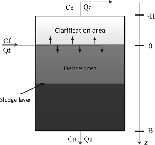
In a unit time, the growth of the arbitrary interval $(z_1,z_2)$ is equal to the flow rate $\left(\mathrm{\Phi }{|}_{z=z_1}\right)$ of the $z_1$ height inflow minus the flow rate of the $z_2$ height flow $\left(\mathrm{\Phi }{|}_{z=z_2}\right)$ plus the flow generated in the interval, and the expression is as shown in Equation (2). (2) $\begin{array}{rl}\frac{\text{d}}{\text{d}t}{\int }_{z_1}^{z_2}AC(z,t)\text{d}z& =A(\mathrm{\Phi }{|}_{z=z_1}-\mathrm{\Phi }{|}_{z=z_2})\\ & +{\int }_{z_1}^{z_2}{Q}_f\left(t\right)C_f\left(t\right)\delta \left(z\right)\text{d}z\end{array}$(2) where $Q_f$ is the feed flow rate; $A$ is the cross-sectional area of the thickener; $C_f$ is the feed concentration; $\delta \left(z\right)$ is the $\delta$ function, $\delta \left(z\right)=1$ only at the feed layer, and at other heights, $\delta \left(z\right)\text{ = 0}$;

Flow $\mathrm{\Phi }$ is expressed as: (3) $\begin{array}{rl}\mathrm{\Phi }\left(C,\frac{\mathrm{\partial }C}{\mathrm{\partial }z},z,t\right)& =F(C,z,t)-\left(\gamma \right(z\left)d{}_{comp}\right(C)\\ & +d_{disp}\left(z\right))\frac{\mathrm{\partial }C}{\mathrm{\partial }z}\end{array}$(3) (4) $\begin{array}{rl}F(C,z,t)& =\left\{\begin{array}{ll}-Q_e\left(t\right)C/A& z<-H\\ v_{hs}\left(C\right)C-Q_e\left(t\right)C/A& -H<z<0\\ v_{hs}\left(C\right)C+Q_u\left(t\right)C/A& 0<z<B\\ +Q_u\left(t\right)C/A& z>B\end{array}\right.\end{array}$(4) (5) $\begin{array}{rl}\gamma \left(z\right)& =\left\{\begin{array}{ll}1& -H\le z\le B\\ 0& z<-H\text{or}z>B\end{array}\right.\end{array}$(5)

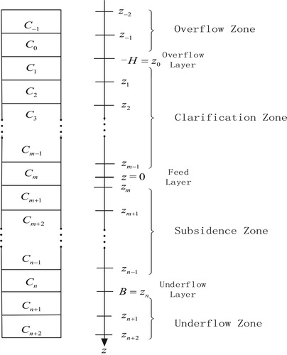
The layering idea (Guo, Zhang, Xu, & Chen, 2009) is used to subdivide the thickener into n layers, so the height of each layer is $\mathrm{\Delta }z=(B+H)/n$. The position of the boundary line between the layers is as shown in Figure 2. The height of each boundary line can be calculated by the formula (6). (6) $z=i\mathrm{\Delta }z-H,i=0,\dots N$(6) The overflow layer $z_0$ and the underflow layer $z_n$ fall on the boundary line; the overflow layer $z_0=-H$, the underflow layer $z_n=B$, and the feeding inlet $z=0$ is in the interval of $\left(z_{m-1},z_m\right]$; and the corresponding m-th layer is the feeding layer. In the simulation scheme, the corresponding overflow zone and the underflow zone are respectively added with two layers at the top and bottom of the equation, the top two layers simulate the overflow zone, and the bottom two layers simulate the underflow zone. The overflow turbidity $C_e$ takes the 0-th layer concentration. The underflow concentration $C_n$ is the n + 1th layer concentration. Therefore, the calculation area consists of n + 4 intervals of length $\mathrm{\Delta }z$.

For each layer, Equation (2) can be rewritten as a simplified version of the mass conservation equation as follows: (7) $\begin{array}{rl}\frac{\text{d}{C}_i}{\text{d}t}& =-\frac{F_i^{num}-F_{i-1}^{num}}{\mathrm{\Delta }z}\\ & +\frac{1}{\mathrm{\Delta }z}(J_{disp,i}^{num}-J_{disp,i-1}^{num}+J_{comp,i}^{num}-J_{comp,i-1}^{num})\\ & +\frac{Q_f{C}_f}{A\mathrm{\Delta }z}{\delta }_{i,m.}i=-1,\dots ,n+2\end{array}$(7) (8) $\begin{array}{rl}{J}_{disp}(z_i,t)& \approx J_{disp,i}^{num}:=J_{disp,i}\frac{C_{i+1}-C_i}{\mathrm{\Delta }z}\end{array}$(8) (9) $\begin{array}{rl}{J}_{comp}(z_i,t)& \approx J_{comp,i}^{num}:=\gamma \left(z_i\right)\frac{D_{i+1}^{num}-D_i^{num}}{\mathrm{\Delta }z}\end{array}$(9) where $D_i^{num}$ is the compression factor.

Figure 2. Layered structure chart.

Since each term of Equation (7) does not exist in every layer, it is necessary to layer to establish more detailed machine differential equations. In the subsidence zone, the i-th (i = 2 … , n−1) layers are given by $\begin{array}{rl}\frac{d{C}_{\text{i}}}{dt}& =\frac{Q_e}{A\mathrm{\Delta }z}(C_{\text{i}+\text{1}}-C_{\text{i}})-\frac{G_i-G_{i-1}}{\mathrm{\Delta }z}\\ & +\frac{\begin{array}{c}{d}_{disp,i}(C_{i+1}-C_i)-d_{disp,i-1}(C_i-C_{i-1})\\ +D_{i+1}^{num}-2D_i^{num}+D_{i-1}^{num}\end{array}}{{\left(\mathrm{\Delta }z\right)}^2}\end{array}$When $i=m$, the layer is the feed layer: $\begin{array}{rl}\frac{d{C}_m}{dt}& =\frac{Q_f}{A\mathrm{\Delta }z}(C_f-C_m)-\frac{G_m-G_{m-1}}{\mathrm{\Delta }z}\\ & +\frac{\begin{array}{c}{d}_{disp,m}(C_{m+1}-C_m)-d_{disp,m-1}(C_m-C_{m-1})\\ +D_{m+1}^{num}-2D_m^{num}+D_{m-1}^{num}\end{array}}{{\left(\mathrm{\Delta }z\right)}^2}\end{array}$For the underflow layer: $\begin{array}{rl}\frac{d{C}_{n+1}}{dt}& =-\frac{Q_u}{A\mathrm{\Delta }z}(C_{n+1}-C_n)+\frac{G_n}{\mathrm{\Delta }z}\\ & +\frac{(D_{n+1}^{num}-D_n^{num})}{{\left(\mathrm{\Delta }z\right)}^2}\end{array}$where $C_f$ is the feed concentration; $D_i^{num}$ is the dispersion coefficient, $n$ is the number of stratified layers; $z$ is the height of the thickener; $z_f$ is the feed height; $v_s$ is the settling velocity; $C$ is the concentration of the pulp; and $G_i$ is given by formula (10). (10) $G_i=G_i(C_i,C_{i+1})=\left\{\begin{array}{ll}\underset{C_{i\le C\le C_{i+1}}}{min}C{v}_{hs}\left(C\right)& C_i\le C_{i+1}\\ \underset{C_{i>C>C_{i+\stackrel{`}{1}}}}{max}C{v}_{hs}\left(C\right)& C_i>C_{i+1}\end{array}\right.$(10)

2.2. Application of Bernoulli principle

Based on the limitations of the field conditions, the flow velocity of the fluid cannot be measured by the instrument. Therefore, the Bernoulli equation (Zhang, 2016) of fluid mechanics is used to convert the pressure data measured by the field instrument into the flow velocity suitable for the mechanism model for subsequent data processing; this approach is of great convenience. At the same time, the gravitational potential energy of the fluid at the same level is ignored, so the formula for the flow rate and pressure of the fluid can be expressed as Equation (11) (11) $v=\sqrt{\frac{2p}{\rho }}$(11) In order to carry out the next simulation analysis, Table 1 gives the model parameters of the dense washing process mechanism model.

Table 1 Parameter set for the mechanism model of the thickener.

Model parameter	Parameter meaning	Parameter values	Unit
$A$	Thickener cross section	1962.5	[m^2]
$z$	Thickener height	5.95	$\left[\text{m}\right]$
Zf	Feed layer height	2.06	$\left[\text{m}\right]$
$r$	Free settlement velocity undetermined parameter 1	1.3359	$[-]$
k0	Free settlement velocity undetermined parameter 2	0.0325	$\left[\text{m/h}\right]$
n0	Free settlement velocity undetermined parameter 3	0.0001785	[m^3/kg]
$k_1$	Undetermined parameters of the velocity of interference settlement 1	6.79	$\left[\text{m/h}\right]$
$n_1$	Undetermined parameters of the velocity of interference settlement 2	0.000425	$\left[{\text{m}}^3\text{/kg}\right]$
k2	Pressure settlement velocity undetermined parameter 1	70.9	$\left[\text{m/h}\right]$
n2	Pressure settlement velocity undetermined parameter 2	0.000875	[m^3/kg]
$\beta$	Settlement function parameter 1	4.00	[kg/m^3]
$\alpha$	Settlement function parameter 2	4.00	$\left[\text{Pa}\right]$
α1	Diffusion function parameter 1	0.001	[m^−1]
α2	Diffusion function parameter 2	0.0026	[s/m^2]
CC	ritical concentration	6.00	[kg/m^3]
$g$	acceleration of gravity	9.81	[m/s^2] [kg/m^3]
${\rho }_s$	Solid density	1050	[kg/m^3]
$\mathrm{\Delta }\rho$	Density difference between solid and liquid	50	[kg/m^3]

2.3. Auxiliary variable selection

Auxiliary variables include the type of variable, the number of variables, and the location of the monitoring point. The choice of auxiliary variables is the first step in establishing a process data model. This step determines the input of the soft-measurement model and thus has a direct impact on the model structure, which is critical to the success of the model. The selection of auxiliary variables is generally through the mechanism analysis, clarifying the task of the soft-measurement model, determining the dominant variables, and selecting the main influencing factors from the measurable variables affecting the dominant variables. The task of the mechanism model in this paper is to predict the underflow concentration of the key variables in the dense washing process to determine the dominant variable of the soft-measurement model as the underflow concentration. Variables that have a large impact on the underflow concentration include top volume flow, feed flow, underflow bulk density, and fluid flow rate. These four variables can be measured by the inspection device at the industrial site, so we choose them as input variables of the model, and choose underflow concentration as output variable of the model. Table 2 is the auxiliary variable.

Table 2. Variable tables.

Order number	Variable name	Variable meaning
1	$x_1$	Top volume flow
2	$x_2$	Underflow bulk density
3	$x_3$	Feed flow
4	$x_4$	Fluid flow rate
5	y	Underflow concentration

2.4. Data preprocessing

In the actual measurement data, there are often individual measurement data that obviously exceed the general range of measurement data, that is, the measurement value is too far from the average level of the remaining measurement values; such data are usually set as an abnormal value. Outliers can usually be processed using the $3\sigma$ principle. In general, for a sample set x, if there is only a random error in the sample, the normal distribution law of the random error is statistically calculated, and the data with the absolute value of the deviation greater than $3\sigma$ are regarded as abnormal data and are eliminated. The specific implementation method is:

For the measurement data $\left[x_1,x_2,x_3,x_4\right]$, the average value is first calculated according to formula (12), and the estimated value of the standard deviation is calculated according to Equation (13). (12) $\begin{array}{rl}\overline{x}& =\frac{1}{n}\sum _{i=1}^n{x}_i\end{array}$(12) (13) $\begin{array}{rl}\sigma & =\sqrt{\frac{1}{n}\sum _{i=1}^n{(x_i-\overline{x})}^2}\end{array}$(13) It is assumed that for any data point $x_d$, if $|x_d-\overline{x}|>3\sigma$ is satisfied, the data is regarded as an outlier according to the $3\sigma$ principle, and $x_d$ should be excluded from the measurement data. After the $x_d$ is removed, the $\sigma$ value is recalculated for the retained data, the outlier detection is repeated, and the iterative operation is repeated until all outliers are eliminated.

2.5. Parameter identification and simulation of mechanism model

Figure 3 shows the recursive least squares (RLS) optimized thickener mechanism model.

Figure 3. Mechanism model parameter identification optimization model.

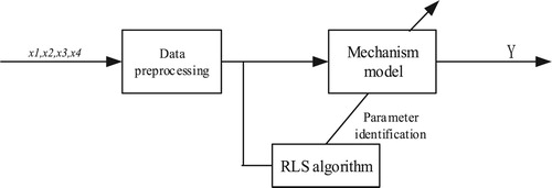
Improve the parameters of the thickener mechanism model, $\begin{array}{r}\frac{d{C}_i}{dt}=g_1\frac{Q_e}{ADz}\text{(}{C}_{i+1}-C_i\text{)}-\frac{G_i-G_{i-1}}{Dz}\\ +\frac{d_{disp,i}\text{(}{C}_{i+1}-C_i\text{)}-d_{disp,i-1}\text{(}{C}_i-C_{i-1}\text{)}+D_{i+1}^{num}-2D_i^{num}+D_{i-1}^{num}}{{\text{(}Dz\text{)}}^2}\\ \frac{d{C}_m}{dt}=g_2\frac{Q_f}{ADz}\text{(}{C}_f-C_m\text{)}-\frac{G_m-G_{m-1}}{Dz}\\ +\frac{\begin{array}{c}{d}_{disp,m}\text{(}{C}_{m+1}-C_m\text{)}-d_{disp,m-1}\text{(}{C}_m-C_{m-1}\text{)}\\ +D_{m+1}^{num}-2D_m^{num}+D_{m-1}^{num}\end{array}}{{\text{(}Dz\text{)}}^2}\\ \frac{d{C}_{n+1}}{dt}=-g_3\frac{Q_u}{ADz}\text{(}{C}_{n+1}-C_n\text{)}+g_4\frac{G_n}{Dz}\\ +\frac{\text{(}{D}_{n+1}^{num}-D_n^{num}\text{)}}{{\text{(}Dz\text{)}}^2}+g_5\end{array}$where $A$ is the cross-sectional area of the thickener, $H$ is used to describe the height of the clarification zone, $B$ is the depth of the settlement zone, $\mathrm{\Delta }z=(B+H)/n$ is the height of each layer, $Q_d$ is the top volume flow rate, $Q_f$ is the feed flow, $Q_u$ is the underflow bulk density, $D_i^{num}$ is the compressibility factor that contains the pulp concentration and density, $G_i$ contains the settling velocity model v, and ${\gamma }_1,{\gamma }_2,{\gamma }_3,{\gamma }_4,{\gamma }_5$ are undetermined parameters.

Fifty sets of data were randomly selected from the 190 sets of data measured in the field to identify the parameters of the RLS identification thickener mechanism model. Table 3 shows the parameters of the mechanism model after identification.

Table 3. Results of RLS parameter identification.

Parameter	${\gamma }_1$	${\gamma }_2$	${\gamma }_3$	${\gamma }_4$	${\gamma }_5$
Identification result	0.2327	0.0293	0.2585	0.7427	0.5155

Figure 4 shows the simulation results of the mechanism model after the RLS parameter identification.

Figure 4. Prediction results of mechanism model. (a) Prediction error of underflow concentration. (b) Prediction effect of underflow concentration.

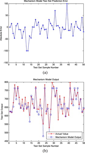
From Figure 4(a), it can be seen that the error of the mechanism model after RLS parameter identification is a bit large. So further modification is needed to make the predicted value of the mechanism model closer to the actual value. Figure 4(b) shows that although the mechanism model of parameter identification has a good predictive effect on the trend of the process, the actual industrial process is often complicated, some factors in the process are constantly changing, and its changes are difficult to accurately describe, leads to large deviations in the prediction results of the model. Thus, the data cannot be applied to the real-time monitoring of industrial field data. As a result, further correction is required to obtain a more accurate prediction effect.

This chapter establishes a mechanism model of slurry concentration distribution in dense washing process based on solid flux theory and mass conservation theory. Then, the Bernoulli principle of fluid mechanics is used to convert the pressure data measured in the field into the flow velocity suitable for the mechanism model, which brings great convenience to the subsequent data processing. Finally, the parameter identification mechanism model of RLS algorithm is adopted. By simulating the mechanism model of parameter identification, the main factors affecting the dense washing process are found out. The mechanism model for measuring the underflow concentration is established, which provides a direction for subsequent optimization.

3. Data model establishment based on TELM

3.1. Introduction of ELM

Extreme Learning Machine (ELM) is a learning algorithm for a single hidden layer feedforward neural networks (SLFNs). In the ELM model, the weights and threshold parameters of the network are given randomly before training, and no iteration correction is needed. It is only to manually select the number of hidden layer nodes. After the least squares operation, the only optimal solution of the ELM network can be obtained without falling into the local optimum.

With the increasing popularity of neural networks, the research and innovation of the algorithm have developed rapidly because of the characteristics of the ELM algorithm (Huang, 2014; Huang, Zhu, & Siew, 2004, 2006). At the same time, there are many studies dedicated to improving ELM. The incremental extreme learning machine (Huang & Chen, 2007, 2008), the error minimum extreme learning machine (Feng & Huang, 2009), the reconstructed hidden layer node extreme learning machine (Lan, Soh, & Huang, 2010), the extreme learning machine for optimal middle-layer node selection (Miche, Sorjamaa, & Bas, 2010), the extreme learning machine with regularization term (Deng, Zheng, & Chen, 2009), the extreme learning machine using integrated learning ideas (Liu & Wang, 2010), and the extreme learning machine combined with deep learning ideas (Ma, 2015). Continuous improvement and development have allowed the ELM algorithm to be successfully applied to all walks of life, especially in the fields of classification, regression, and pattern recognition.

Figure 5 shows the ELM network structure in which neurons are connected together in adjacent network layers in the network. The input layer have $n$ number of neuron nodes, and there are $n$ dimensions corresponding to one input data sample. The number of hidden layer neuron nodes is $l$, which are randomly set by experience. The output layer has $m$ neurons nodes.

Figure 5. The network structure of the ELM.

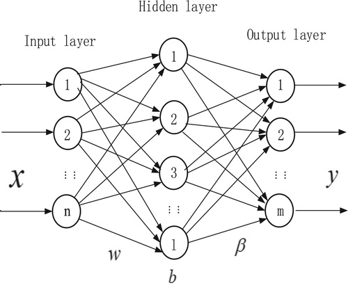
Equation (14) gives the connection weight matrix $w$ between the input layer and the hidden layer. (14) $w={\left[\begin{array}{cccc}{w}_{11}& w_{12}& \cdots & w_{1n}\\ w_{21}& w_{22}& \cdots & w_{2n}\\ ⋮& ⋮& & \\ w_{l1}& w_{l2}& \cdots & w_{ln}\end{array}\right]}_{l\times n}$(14) where $w_{ji}$ represents the connection weight between the j-th neuron in the hidden layer and the i-thneuron in the input layer.

Let the connection weight $\beta$ between the output layer and the hidden layer be: (15) $\beta ={\left[\begin{array}{cccc}{\beta }_{11}& {\beta }_{12}& \cdots & {\beta }_{1m}\\ {\beta }_{21}& {\beta }_{22}& \cdots & {\beta }_{2m}\\ ⋮& ⋮& & \\ {\beta }_{l1}& {\beta }_{l2}& \cdots & {\beta }_{lm}\end{array}\right]}_{l\times m}$(15) where ${\beta }_{jk}$ represents the connection weight between the k-th neuron of the output layer and the j-th neuron of the hidden layer.

The hidden layer threshold $b$ is given by Equation (16) (16) $b={\left[\begin{array}{c}{b}_1\\ b_2\\ ⋮\\ b_l\end{array}\right]}_{l\times 1}$(16) Suppose the input matrix with $Q$ training set samples is $X(n\times Q)$ and the marking matrix is $Y(m\times Q)$. (17) $\begin{array}{c}X=\left[\begin{array}{cccc}{x}_{11}& x_{12}& \cdots & x_{1Q}\\ x_{21}& x_{22}& \cdots & x_{2Q}\\ ⋮& ⋮& & \\ x_{n1}& x_{n2}& \cdots & x_{nQ}\end{array}\right]\\ Y=\left[\begin{array}{cccc}{y}_{11}& y_{12}& \cdots & y_{mQ}\\ y_{21}& y_{22}& \cdots & y_{mQ}\\ ⋮& ⋮& & \\ y_{m1}& y_{m2}& \cdots & y_{mQ}\end{array}\right]\end{array}$(17) ELM output is $T={\left[\begin{array}{cccc}{t}_1& t_2& \cdots & t_Q\end{array}\right]}_{m\times Q}$ (18) $t_j={\left[\begin{array}{c}{t}_{1j}\\ t_{2j}\\ ⋮\\ t_{mj}\end{array}\right]}_{m\times 1}=\begin{array}{c}{\left[\begin{array}{c}\sum _{i=1}^l{\beta }_{i1}g(w_i{x}_j+b_i)\\ \sum _{i=1}^l{\beta }_{i2}g(w_i{x}_j+b_i)\\ ⋮\\ \sum _{i=1}^l{\beta }_{im}g(w_i{x}_j+b_i)\end{array}\right]}_{m\times 1}\\ j=1,2,\dots ,Q\end{array}$(18) where $w_i=\left[\begin{array}{cccc}{w}_{i1}& w_{i2}& \dots & w_{in}\end{array}\right]$, $x_j=[\begin{array}{cccc}{x}_{1j}& x_{2j}& \dots & x_{nj}\end{array}{]}^{T}g\left(x\right)$ is activation function.

Equation (18) can also be expressed as (19) $H\beta =T^{\mathrm{\prime }}$(19) where $H$ is the output matrix of the ELM hidden layer, $H={\left[\begin{array}{ccc}g(w_1{x}_1+b_1)& \cdots & g(w_l{x}_1+b_l)\\ ⋮& \ddots & ⋮\\ g(w_1{x}_Q+b_1)& \cdots & g(w_l{x}_Q+b_l)\end{array}\right]}_{Q\times l}$and $T^{\mathrm{\prime }}$ is the transpose of the tag matrix $T$.

Then the output weight can be obtained from Equation (20). (20) $\beta =H^{+}T$(20) where $H^{+}$is the Moore-Penrose generalized inverse of the output matrix $H$.

Thus, the output of the ELM network is $y=H\beta$.

3.2. Selection of activation function and the number of hidden layer nodes

In artificial neural networks, the activation function has a huge impact on the model. Since the data set processed by the neural network may have low nonlinearity and affect the training of the model, it is necessary to add an activation function to improve the nonlinearity of the model. When the activation function is a linear function, the final output and the input must also be linear, so that the hidden layer in the network does not reflect the value of its hidden layer, so the activation function needs to use nonlinear function. At the same time, when the expression ability of linear data is weak, the expression ability of the model can be improved by adding nonlinear factors by adding an activation function.

A suitable activation function can improve performance of the ELM. The activation function must satisfy conditions such as nonlinearity, differentiability, and monotonicity.

Some commonly used activation functions and their mathematical expressions are as follows:

• Sigmoid function: $g\left(x\right)=1/(1+e^{-x})$

• Linear function: $g\left(x\right)=kx+c$

• ReLU: $g\left(x\right)=max(x,0)$

• Sinusoidal function: $g\left(x\right)=\sin \left(x\right)$

• Log function: $g\left(x\right)=\ln \left(x\right)$

• Hyperbolic tangent function: $g\left(x\right)=\frac{e^x-e^{-x}}{e^x+e^{-x}}$

• Hardlim function: $g\left(x\right)=\left\{\begin{array}{l}\text{1},x\ge \text{0}\\ \text{0},x<0\end{array}\right.$

• Polynomial function:

• $g\left(x\right)=\text{0}\text{.1}\times (e^x+x^2\cos (x^2)+x^2)$

• Radbas function:$g\left(x\right)=e^{-n^2}$

• Satlin function: $g\left(x\right)=\left\{\begin{array}{l}\text{1},x\ge 1\\ x,0<x<1\\ 0,x<0\end{array}\right.$

At present, there is no definitive method to select the number of neuron nodes in the hidden layer of the artificial network. Most scholars have conducted experiments based on their own experience and selected the best results. We also determined the number of neuron nodes in the hidden layer by the method of ‘optimizing from multiple training’.

3.3. Introduction of TELM

The limit learning machine of the three hidden layer network structure (TELM) (Xiao, Li, & Mao, 2017) adds two hidden layers on the basis of the classical extreme learning machine, and each layer of neurons is in a fully connected state. At the same time, the algorithm inherits the advantage of the ELM algorithm to randomly initialize the first hidden layer parameter, and introduces a method to obtain the parameters of the other hidden layer. The method passes the layer-by-layer transmission of network parameters between different hidden layers, and the final output is closer to the actual result than the traditional ELM model, and also inherits the advantages of the traditional extreme learning machine.

Figure 6 is the network structure and algorithm flow of TELM.

Figure 6. TELM flow and structure. (a) The work flow of the TELM. (b) The structure of the TELM.

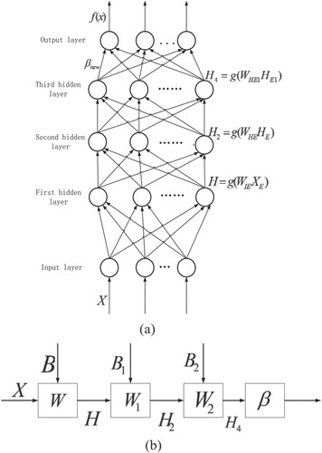
 Suppose a given input training set sample is $\{X,T\}=\{x_i,t_i\}(i=1,2,\dots ,Q)$, where $X$ is the input sample and $T$ is the flag sample. According to the TELM algorithm, we first consider the three hidden layers in the TELM network as two hidden layers (the latter two hidden layers as an implicit layer). The weight matrix of the first hidden layer and the threshold parameters are randomly initialized. It can be known from the ELM algorithm that the expected output of the third hidden layer can be obtained by Equation (21). (21) $H_{3\ast }=T{\beta }_{new}^{+}$(21) where ${\beta }_{new}^{+}$ is the generalized inverse matrix of ${\beta }_{new}$.

Next, the third hidden layer of the network is added. The predicted output $H_3$ of the third hidden layer is given by Equation (22). (22) $H_3=g(W_2{H}_2+B_2)$(22) where $W_2$ is the weight matrix between the second hidden layer and the third hidden layer, $B_2$ is the threshold of the third hidden layer, and $H_2$ is the output matrix of the hidden layer and is given here as the second implicit output matrix of the layer.

Make the predicted output of the third hidden layer infinitely close to the expected output for $H_3=H_{3^{\ast }}$.

We assume the matrix $W_{HE1}=\left[B_2{W}_2\right]$; thus, the weight $W_2$ and threshold $B_2$ of the third hidden layer can be solved by Equation (23). (23) $W_{HE1}=g^{-1}\left(H_{3\ast }\right)H_{E1}^{+}$(23) where $H_{E1}^{+}$ is the generalized inverse matrix of matrix $H_{E1}=[\begin{array}{cc}1& H_2\end{array}{]}^T$, 1 represents a vector with $Q$ elements and each element is 1, and $g^{-1}\left(x\right)$ is the inverse of activation function $g\left(x\right)$.

The predicted output of the third hidden layer can be updated by Equation (24) (24) $H_4=g(W_2{H}_2+B_2)=g\left(W_{HE1}{H}_{E1}\right)$(24) Then ${\beta }_{new}$ can be updated by Equation (25). (25) ${\beta }_{new1}=H_4^{+}T$(25) The TELM neural network output$f\left(x\right)$ can be finally obtained by Equation (26). (26) $f\left(x\right)=H_4{\beta }_{new1}$(26)

3.4. Data model establishment and simulation

Data modeling is to find out the relationship between input and output by performing data processing and statistical analysis on the historical data of the controlled process. Data modeling does not require knowing the specific process to avoid complex mechanism analysis. It only needs to determine the input and output of the model, so it is convenient.

The data collected from the industrial site is processed, and 140 sets of data are randomly selected from the 190 sets of data as training set data, 50 sets of data are used as test set data. Use the TELM algorithm to build a data model.

Figure 7(a) shows that the error of the predicted value generated by the simple data model still has a certain deviation from the actual value; thus, the predicted data don’t meet the actual measurement requirements of the industrial site, and the data model needs further optimization. Figure 7(b) shows the output of the data model. A certain deviation between the predicted output of the data model and the actual value is found. Because the data model only depends on the process data, the information source is single and cannot reflect the process characteristics. The structure of the data model has great subjectivity, resulting in poor generalization, and the model is not explanatory; moreover, it is easy to cause over-fitting phenomenon and predictive output inaccuracy.

Figure 7. Prediction results of data model. (a) Prediction error of TELM test set. (b) TELM test set output comparison.

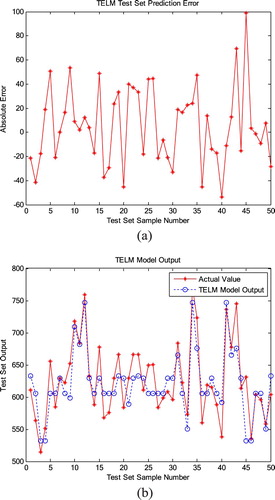
In this chapter, after pre-processing the data collected at the process site, a data model is established. Through simulation analysis, it can be seen that the establishment of the data model avoids the analysis of complex mechanisms, and only needs to determine the input and output of the model and the solution of the model is very convenient. However, because it only relies on process data and the data source is single, the simulation results still have certain deviations from the actual ones, which can not meet the measurement requirements of the industrial site, but provide a clear direction for the establishment and optimization of the next hybrid model.

4. Establishment of a hybrid model

The advantage of mechanism modeling is to reflect the law of the process, high reliability, good extrapolation and interpretability. The disadvantage is that the modeling process is cumbersome and relies on prior knowledge. For some complex processes, reasonable assumptions are needed to obtain a simplified model of the controlled process. However, the accuracy of the simplified mechanism model cannot be guaranteed. The advantage of data modeling is that the process model can be directly established according to the input and output data of the process, without the prior knowledge of the process object, and avoiding the analysis of complex mechanisms. The disadvantage is that the model has poor performance, is not interpretable, easily causes over-fitting, and may even fit in the noise, resulting in instability of the model. In summary, the use of a mechanistic model alone or a separate data model has significant drawbacks. Therefore, this paper proposes a method of combining mechanism modeling and data-driven modeling, so that the mechanism model and the data model can complement each other.

The data compensation model based on the EDO-TELM algorithm combined with the mechanism model of the thick washing process constitutes a hybrid model of the dense washing process, as shown in Figure 8. The model uses a mechanism model to describe the overall characteristics of the dense washing process. As the error compensation model of the mechanism model, the data model establishes the relationship between the deviation of the mechanism model and the process measurable variables. The error generated by the mechanism model is taken as the output of the data model, and the input data is used as an input sample to train the compensator, that is, the EDO-TELM model. The mechanism model is added to the predicted value of the compensator as the estimated value of the model. Therefore, EDO-TELM is used to compensate the deviation of the mechanism model, that is, EDO-TELM is used to compensate the error of the un-modeled part, and the uncertain part of the model is given a reasonable estimate, which greatly reduces the model error. The prediction accuracy of the model is improved.

Figure 8. Hybrid model structure of dense washing process.

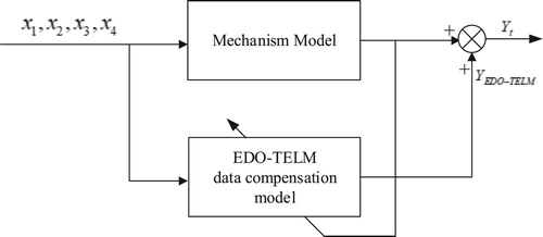
The input and output relationship of the hybrid model can be expressed as follows: (27) $\begin{array}{r}{Y}_t=Y_m\left(x_1,x_2,x_3,x_4\right)+Y_{EDO-TELM}\left(x_1,x_2,x_3,x_4\right)\end{array}$(27) In the formula, $x_1,x_2,x_3,x_4$ represents four measurable auxiliary variables; function $Y_m\left(x_1,x_2,x_3,x_4\right)$ represents the predicted output of the mechanism model; function $Y_{EDO-TELM}\left(x_1,x_2,x_3,x_4\right)$ represents the compensation value of the EDO-TELM compensation model for the output error of the mechanism model; $Y_t$ represents the predicted output of the hybrid model, that is, the model estimate.

4.1. Introduction of EDO

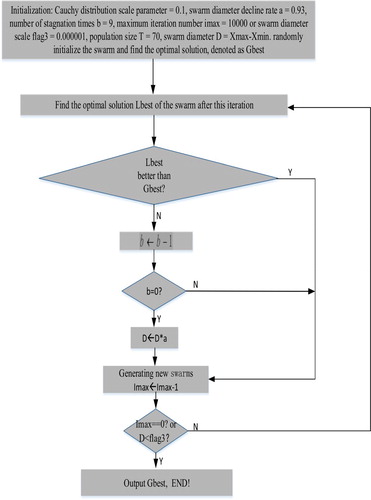
The entire distribution optimization algorithm (Xue, Liu, & Xiao, 2015) (EDO) is a new optimization algorithm derived from the PSO (Chen, 2017) algorithm, which is based on summarizing the population distribution law of the PSO algorithm. Compared with the PSO algorithm, it has the characteristics of simple implementation, fast convergence and strong robustness. Figure 9 shows the specific calculation process.

Figure 9. Program flow chart of EDO.

4.2. TELM optimized with EDO

In the process of optimizing the three-layer extreme learning machine (EDO-TELM) in the overall distribution optimization algorithm, the position of each particle in the EDO algorithm corresponds to the input weight and offset vector of the TELM. The dimension of the particle is determined by the number of input layer and first hidden layer neurons, and the training set output error is used as the fitness value. The particle swarm searches for input weights and offset vectors that minimize the TELM output error by moving the search within the weight space.

The steps of EDO optimization algorithm optimizes the TELM as follows:

In this paper, the specific implementation steps of optimizing the TELM by using the EDO algorithm are as follows:

Step 1: Initialize the TELM: S Set the number of input and output neurons in the network and select the appropriate activation function.

Step 2: Initialize the EDO: Randomly generate the swarm within the entire domain while initializing the Cauchy distribution to cover a radius of 0.5 times the entire domain. Set the following parameters: Cauchy distribution scale parameter r = 0.1, swarm diameter decline rate a = 0.93, number of stagnation times b = 9, maximum iteration number 10,000 or swarm diameter scale less than 0.000001, and swarm size 70.

Step 3: Calculate the fitness value: For all the particles, using the TELM model, calculate their respective output values and finally obtain the sample error; the sample error is the fitness of each particle.

Determine whether the maximum number of iterations is reached, or whether the fitness value meets the requirements, if the condition is satisfied, go to the step 6, otherwise continue to execute downward;

Step 4: Update the global extremum and the individual extremum of each particle: the best individual of this time is compared with the last best individual; if it is better than the last best individual, then replace the last optimal individual, As the optimal individual of this time, the swarm diameter remains unchanged; if it is worse than the last optimal individual, then the last optimal individual is retained as the optimal individual of this time, and the number of stagnation times is reduced by one. If the number of stagnation times is 0, then the swarm diameter is reduced to 0.93 of the original diameter, and the number of stagnation times is set to 9. If the number of stagnation times is not 0, then the original diameter remains unchanged. The number of iterations is reduced by 1.

Step 5: Focus on the location of the best individual found, and then generate a new swarm with the Cauchy distribution.

Step 6: When the maximum number of iterations is reached or the scale of the swarm diameter is less than 0.000001, the algorithm stops iteratively, and the input weight and offset vector of the TELM corresponding to the global extremum are the optimal solution of the problem. An excellent solution and input test samples for forecasting are obtained.

4.3. Simulation and analysis of hybrid models

The field measured input variables $x_1,x_2,x_3,x_4$ (that is $Q_{\epsilon },Q_f,Q_u,Q_v$) are selected to compare the predicted output of the mechanism model, the data model and the hybrid model. The predicted result is the underflow concentration, and compare the prediction errors. The following three tables are numerical comparisons of selected data for the experimental results.

It can be seen from Table 4 (Panel A) that the error of the mechanism model after parameter identification is large, among them, the maximum error rate is more than 10%, indicating that the pure mechanism model is not suitable for complex industrial processes and needs to be combined with other modeling methods. Table 4 (Panel B) shows that the prediction error of the data model is also relatively large and cannot be adapted to the needs of industrial field measurement. The data in Table 4 (Panel C) shows that the predicted value of the hybrid model is approaching the actual value, and the error rate is about 5%, which is 5 percentage points higher than the accuracy of the mechanism model, which meets the measurement needs of complex industrial sites.

Table 4. Comparison of predicted and actual values under three models.

Panel A. Mechanism model predictive output compared with actual values ($\text{unit}\text{:kg/}{\text{m}}^{\text{3}}$)
Actual value	783	796	619	615	568	576	633	666	678	646	568	547	666	564
Predicted value	823.6	841.9	654.2	650.8	613.3	616.6	89.6	733.5	712.3	690.1	613.3	584.5	733.5	615.1
Error	40.6	45.9	35.2	35.8	45.3	40.6	56.6	67.5	34.3	44.1	45.3	37.5	67.5	51.1
Error rate	0.052	0.058	0.057	0.058	0.08	0.071	0.089	0.101	0.051	0.068	0.074	0.064	0.092	0.083
Panel B. Data model predictive output compared with actual values ($\text{unit}\text{:kg/}{\text{m}}^{\text{3}}$)
Actual value	783	796	619	615	568	576	633	666	678	646	568	547	666	564
Predicted value	823.6	841.9	654.2	650.8	613.3	616.6	689.6	733.5	712.3	690.1	613.3	584.5	733.5	615.1
Error	40.6	45.9	35.2	35.8	45.3	40.6	56.6	67.5	34.3	44.1	45.3	37.5	67.5	51.1
Error rate	0.052	0.058	0.057	0.058	0.08	0.071	0.089	0.101	0.051	0.068	0.074	0.064	0.092	0.083
Panel C. Hybrid model predictive output compared with actual values ($\text{unit}\text{:kg/}{\text{m}}^{\text{3}}$)
Actual value	709	646	619	611	622	718	666	712	736	696	604	529	622	596
Predicted value	732.4	668.1	641.5	603.0	630.9	720.4	656.6	717.4	746.9	712.7	596.9	556.6	630.9	605.0
Error	23.4	22.1	22.5	−8.0	8.9	2.4	−9.4	5.44	10.9	16.7	−7.1	27.6	8.9	9.0
Error rate	0.033	0.034	0.036	−0.01	0.014	0.003	−0.01	0.008	0.015	0.024	−0.01	0.052	0.014	0.015

In order to verify the prediction effect of the hybrid model, 190 data generated by the mechanism model was used for simulation. Among them, 130 groups were used as training samples and 60 groups were used as test samples. Figure 10 shows the simulation results.

Figure 10. Prediction results of hybrid model. (a) Prediction error of underflow concentration. (b) Predictio of underflow concentration.

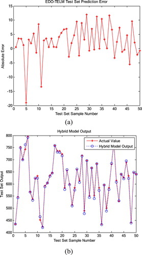
Figure 10(a) shows the prediction error of the hybrid model. the prediction error is below 2% and the prediction accuracy is significantly improved. Figure 10(b) is the output of the predicted value of the hybrid model. It can be seen that the predicted and actual values of the hybrid model are very close. The hybrid model can compensate for the deviation of the mechanism model, and the prediction effect is better and the precision is higher, which can meet the actual production requirements.

In this section, the EDO algorithm is used to optimize the parameters of the first hidden layer of TELM. A method combining the mechanism model and the modeling based on EDO-TELM data compensation model is proposed. The experimental results show that the hybrid model achieves an accurate prediction of the underflow concentration of the thickener, which can meet the measurement requirements of the underflow concentration of the thickener in complex industrial production.

5. Conclusion

For the prediction of the underflow concentration in the thick washing process, this paper uses the hybrid modeling method to establish a soft measurement model of the dense washing process, which is composed of the optimized mechanism model and the data compensation model. The mechanism model is used to describe the overall trend of the dense washing process and reduce the amount of calculation of the model. The data model is used to compensate for errors in the mechanism model. Considering the nonlinear characteristics of the thick washing process, the mechanism model is parameterized to improve the accuracy of the mechanism model modeling. The data compensation model uses the improved EDO-TELM algorithm. In this paper, the mechanism model, mathematical model and hybrid model are simulated respectively. Simulation results prove that compared with the mechanism model and the data model, the hybrid model with higher prediction accuracy.

Disclosure statement

No potential conflict of interest was reported by the authors.

Additional information

Funding

This research work is supported by National Natural Science Foundation of China [grant numbers 41371437, 61203214, 61473072, 61773105, 61374147 and 61733003]; Fundamental Research Funds for the Central Universities [grant numbers N180404012, N180704013, N182608003, N150402001, N160404008 and N172410005-7]; National Key Research and Development Plan [grant number 2016YFC0801602]; National Training Program of Innovation and Entrepreneurship for Undergraduates [grant number 201810145161]. National Twelfth Five-Year Plan for Science and Technology Support (2015BAB15B01) PR China. Fundamental Research Funds for Liaoning Natural Science Foundation (Grant No. 2019-MS-120).

References

- Ardabili, S. F., Najafi, B., Shmshirband, S., Bidgoli, M. B., Deo, R. C., & Chau, K. (2018). Computational intelligence approach for modeling hydrogen production: A review. Engineering Applications of Computational Fluid Mechanics, 12(1), 438–458. doi: 10.1080/19942060.2018.1452296
- Bürger, R., Concha, F., Karlsen, K., & Narváez, A. (2006). Numerical simulation of clarifier-thickener units handling of the ideal suspensions with a flux density function having two inflection points. Mathematical and Computer Modelling, 44, 255–275. doi: 10.1016/j.mcm.2005.11.008
- Bürger, R., Diehl, S., Farås, S., Nopens, I., & Torfs, E. (2012). A consistent modeling methodology for secondary settling tanks: A reliable numerical method. Water Research, 46(2), 2254–2278.
- Bürger, R., Diehl, S., & Nopens, I. (2011). A consistent modelling methodology for secondary settling tanks in wastewater treatment. Water Research, 45, 2247–2260. doi: 10.1016/j.watres.2011.01.020
- Chen, J. Q. (2017). Compression perception based on improved particle swarm optimization. Signal Processing Device, 33(4), 488–495.
- Deng, W. Y., Zheng, Q. H., & Chen, L. (2009). Regularized extreme learning machine. 2009 IEEE symposium on computational intelligence and data mining, Nashville, TN, USA.
- Feng, G., & Huang, G. B. (2009). Error minimized extreme learning machine with growth of hidden nodes and incremental learning. IEEE Transactions on Neural Networks, 20(8), 1352–1357. doi: 10.1109/TNN.2009.2024147
- Ghalandari, M., Elaheh, M. K., Fatemeh, M., Shahabbodin, S., & Chau, K. (2019). Numerical simulation of nanofluid flow inside root canal. Engineering Applications of Computational Fluid Mechanics, 13(1), 254–264. 2019. doi: 10.1080/19942060.2019.1578696
- Gui, W. H., Yang, C. H., Chen, X. F., & Wang, Y. L. (2013). Problems and challenges in modeling and optimization of non-ferrous metallurgical processes. Acta Automatica Sinica, 39(3), 197–207. doi: 10.1016/S1874-1029(13)60022-1
- Gui, J. L., & Zhao, F. G. (2007). Application of high-efficiency deep cone thickener in Meishan concentrator. Mining Express, 3, 70–71.
- Guo, L. S., Zhang, D. J., Xu, D. Y., & Chen, Y. (2009). An experimental study of low concentration sludge settling velocity under turbulent condition. Water Research, 43(3), 2383–2390. doi: 10.1016/j.watres.2009.02.032
- Huang, G. B. (2014). An insight into extreme learning machines: Random neurons, random features and kernels. Cognitive Computation, 6(3), 376–390. doi: 10.1007/s12559-014-9255-2
- Huang, G. B., & Chen, L. (2007). Convexin cremental extreme learning machine. Neurocomputing, 70(3), 3056–3062. doi: 10.1016/j.neucom.2007.02.009
- Huang, G. B., & Chen, L. (2008). Enhanced random search based incremental extreme learning machine. Neurocomputing, 71(3), 3060–3068.
- Huang, G. B., Zhu, Q. Y., & Siew, C. K. (2004). Extreme learning machine: A new learning scheme of feed forward neural networks. 2004 IEEE International Joint Conference on Neural Networks, 2(2), 985–990. doi: 10.1109/IJCNN.2004.1380068
- Huang, G. B., Zhu, Q. Y., & Siew, C. K. (2006). Extreme learning machine: Theory and applications. Neurocomputing, 70(1), 489–501. doi: 10.1016/j.neucom.2005.12.126
- Ichiro Tetsuo, etc. (1986). Water treatment engineering theory and application. Beijing: China Building Industry Press. (pp. 60–100).
- Kynch, G. J. (1952). A theory of sedimentation. Transactions of the Faraday Society, 48(7), 166–176. doi: 10.1039/tf9524800166
- Lan, Y., Soh, Y. C., & Huang, G. B. (2010). Constructive hidden nodes selection of extreme learning machine for regression. Neurocomputing, 10(16), 5–22.
- Li, Z. L. (2006). One-dimensional flux model of secondary settling tank and its application. Chongqing: Chongqing University.
- Liu, X. D. (2007). Application of interface detector in mud layer of sedimentation tank. Automatic Instrument and Instrument, 1, 52–53.
- Liu, N., & Wang, H. (2010). Ensemble based extreme learning machine. IEEE Signal Processing Letters, 17(8), 754–757. doi: 10.1109/LSP.2010.2053356
- Ma, M. M. (2015). Research on algorithm of ultimate learning machine based on deep learning. Shandong: ocean University of China.
- Ma, X. X. (2004). Study on the treatment of acidic water in high-concentration mines with high-efficiency thickener. China Mine Engineering, 33(5), 17–19.
- Ma, S. J., & Cui, S. T. (2013). Application of mine automatic thickening machine automatic equalizing system. Science & Technology Information, 2, 77.
- Miao, T. Y., Wang, X., Wang, Q. K., & Mao, X. (2009). Research and application of automatic control of thickener production process in wastewater treatment process. Digital Technology and Application, 9(5), 18–20.
- Miche, Y., Sorjamaa, A., & Bas, P. (2010). OP-ELM: Optimally Pruned Extreme Learning Machine. IEEE Transactions on Neural Networks, 21(1), 158–162. doi: 10.1109/TNN.2009.2036259
- Ramezanizadeh, M., Nazari, M. A., Ahmadi, M. H., & Chau, K. (2019). Experimental and numerical analysis of a nanofluidic thermosyphon heat exchanger. Engineering Applications of Computational Fluid Mechanics, 13(1), 40–47. doi: 10.1080/19942060.2018.1518272
- Taormina, R., & Chau, K. W. (2015). Data-driven input variable selection for rainfall-runoff modeling using binary-coded particle swarm optimization and extreme learning Machines. Journal of Hydrology, 529(3), 1617–1632. doi: 10.1016/j.jhydrol.2015.08.022
- Wang, F. L., He, D. K., & Chang, Y. Q. (2012). 2012 implementation report of comprehensive intelligent integrated optimization control technology for hydrometallurgy. Shenyang, China: Northeastern University.
- Xiao, D., Li, B. J., & Mao, Y. C. (2017). A multiple hidden layers extreme learning machine method and its application. Mathematical Problems in Engineering, 2017, 10.
- Xue, C. P., Liu, J. Y., & Xiao, D. (2015). Based on greedy strategy overall distribution optimization algorithm solving 0-1 knapsack problem. Journal of Northeast Normal University, 2015(2), 53–57.
- Yang, H., & Chen, W. (2002). Automatic control of 50m large thickener. Metal Mines, 318(12), 38–40.
- Yaseen, Z. M., Sulaiman, S. O., Deo, R. C., & Chau, K. (2019). An enhanced extreme learning machine model for river flow forecasting: State-of-the-art, practical applications in water resource engineering area and future research direction. Journal of Hydrology, 569, 387–408. doi: 10.1016/j.jhydrol.2018.11.069
- Zhang, L. (2016). Talking about the application of Bernoulli’s equation in fluid mechanics. Education Education Forum, 28.