Numerical study of the hydrodynamic parameters influencing internal corrosion in pipelines for different elbow flow configurations

Abstract

Oil–water two-phase flow is common in the ocean engineering, petroleum, and chemical industries, among others. In the transportation process, the elbow system – as a paramount component – usually suffers from internal corrosion. In order to investigate the corrosion-prone characteristics of elbow systems, the volume of fluid (VOF) method and the renormalization group (RNG) k-ε model were used to study the oil–water flow in three different elbow configurations. The results indicate that the maximum wall shear stress and mass transfer coefficient are located at the intrados of the elbow for all flow configurations. Nevertheless, for horizontal-upward and horizontal-horizontal elbow flows, water does not come into direct contact with the intrados of the elbow, meaning it is much less susceptible to corrosion. Thus, a multiparameter model which also takes into account the water-volume fraction is necessary for characterizing the corrosion process. When this was combined with an analysis of the water wetting process, the horizontal-downward elbow flow was found to exhibit the largest corrosion risk among the three configurations examined, the horizontal-upward elbow flow was the least susceptible and the horizontal-horizontal elbow flow was in the middle.

KEYWORDS:

• Numerical simulation
• elbow flow
• water wetting
• internal corrosion

Nomenclature

$\rho$	=	Mixture density
$\mathrm{\nabla }p$	=	Pressure gradient
$\mathbf{g}$	=	Acceleration of gravity
$\mu$	=	Mixture viscosity
$\mathbf{F}$	=	Continuous surface tension
${\rho }_o$	=	Density of oil phase
${\rho }_w$	=	Density of water phase
${\alpha }_o$	=	Volume fraction of oil phase
${\alpha }_w$	=	Volume fraction of water phase
${\mu }_w$	=	Water phase viscosity
${\mu }_o$	=	Oil phase viscosity
$\sigma$	=	Coefficient of surface tension
$\kappa$	=	Curvature
$\mathbf{n}$	=	Surface normal vector
$\hat{n}$	=	Unit vector
$\hat{n}w$	=	Unit normal vector
$\hat{t}w$	=	Unit tangent vector
$\theta w$	=	Contact angle
$G_k$	=	Generation of turbulent kinetic energy due to mean velocity gradient
$G_b$	=	Generation of turbulent kinetic energy due to buoyancy
$Y_M$	=	Contribution of fluctuating dilatation in compressible turbulence to overall dissipation in compressible turbulence affecting overall dissipation rate
$S_k$	=	User-defined source term
$S_{\epsilon }$	=	User-defined source term
$k$	=	Turbulent kinetic energy
$\epsilon$	=	Turbulent dissipation rate
${\alpha }_k$	=	Inverse effective Prandtl number for k
${\alpha }_{\epsilon }$	=	Inverse effective Prandtl number for ε
C1ε	=	Coefficient in ε equation
C2ε	=	Coefficient in ε equation
C3ε	=	Coefficient in ε equation
$\text{Re}$	=	Reynolds number
$Sc$	=	Schmidt number
$Sh$	=	Sherwood number
$k_m$	=	Mass transfer coefficient
$D$	=	Diffusion coefficient
$d$	=	Hydraulic diameter
$v$	=	Kinematic viscosity
$R$	=	Gas constant
$T$	=	Absolute temperature
$F$	=	Faraday’s constant
${\lambda }_o$	=	Ionic conductivity
$C$	=	Cation concentration
$Z_o$	=	Ionic valence
$v_{+}$	=	Number of cations per formula unit of charge carrier
$\delta$	=	Water layer thickness

1. Introduction

Oil and water immiscible two-phase flows are widely used in the petroleum, chemical, and oil and gas transportation industries. When corrosive agents such as CO₂, NH₃, and H₂S dissolve into water, they form corrosive solutions (Kermani & Morshed, 2003; Magnini, Ullmann, Brauner, & Thome, 2018; Pouraria, Seo, & Paik, 2016b; Xu, 2007). When these corrosive solutions come into contact with the internal surfaces of pipelines, a strong electrochemical reaction takes place which can result in severe internal corrosion over time (Nešić, 2007; Zhang, Wang, Wang, & Han, 2012). A large number of numerical simulations and experimental studies have been carried out in order to better understand the mechanism of wall thinning and other problems within pipelines related to corrosion, and it has been proposed that the wall shear stress and mass transfer coefficient can be used to predict where corrosion in pipelines due to erosion will occur (Hu & Cheng, 2016; Pietralik & Schefski, 2009; Pietralik & Smith, 2006; Utanohara & Murase, 2019; Zhang, Zeng, Huang, & Guo, 2013; Zheng & Che, 2006). A summary of previous studies conducted on pipelines with diameters ranging from 14 to 105 mm which use the wall shear stress and mass transfer coefficient hydrodynamic parameters for predicting the corrosion process is presented in Table 1. It can be seen that most of the studies predict the corrosion process using either the wall shear stress or the mass transfer coefficient, and that they usually concentrate on single-phase flow. Furthermore, the pipe configurations are simple; horizontal-upward and horizontal-downward arrangements were mostly adopted, which do not take into account the variations that occur in pipeline layouts in the real world.

Table 1. Summary of the hydrodynamic parameters used to predict elbow flow corrosion.

Authors	Media	Diameter (mm)	Hydrodynamic parameter(s)	Corrosion location	Configuration
Pietralik and Smith (2006)	Water	59	Mass transfer coefficient	Intrados bend	Horizontal-horizontal
Pietralik and Schefski (2009)	Water	38	Mass transfer coefficient	Intrados bend	Horizontal-horizontal
El-Gammal et al. (2010)	Water	40	Velocity	Intrados bend	Horizontal-upward
Zhang et al. (2013)	Water	50	Wall shear stress	Intrados bend	Horizontal-downward
Rani, Divya, Sahaya, Kain, and Barua (2014)	Water	34	Wall shear stress; mass transfer coefficient	Intrados bend	Horizontal-upward
Lin and Ferng (2014)	Water	70	Wall shear stress	Intrados bend	Horizontal-upward
Keshtkar et al. (2016)	Water	105	Mass transfer coefficient	Intrados bend	Horizontal-horizontal
Magnini et al. (2018)	Water	33	Wall shear stress; mass transfer coefficient	Intrados bend	Horizontal-downward
Prasad et al. (2018)	Water	14	Mass transfer coefficient	Extrados bend	Horizontal-downward
Ajmal et al. (2019)	Water	63	Wall shear stress	Intrados bend	Horizontal-downward
Zheng and Che (2006)	Gas–water	35	Wall shear stress; mass transfer coefficient	Vertical pipe	Vertical-downward
Hu and Cheng (2016)	Oil–water	102	Wall shear stress	Intrados incline pipe	Horizontal-upward incline
Zhang et al. (2019)	Oil–water	100	Wall shear stress	Intrados incline pipe	Horizontal-upward incline
Tang, Yang, Zheng, and Wong (2009)	Oil–gas–water	19	Wall shear stress	Straight pipe	Horizontal flow

When contrasted with the single-phase aqueous solution, the addition of the oil phase makes the corrosion mechanism more complex. Extensive study of the corrosion mechanism in oil–water two-phase flow has related the occurrence of water wetting to the formation of corrosion. However, many factors can affect the process of water wetting, including the water cut, pipe diameter, fluid velocity, pipe angle of inclination, oil properties, surface tension, inhibitors, roughness, temperature, and so on (Cai & Nesic, 2004; Chen et al., 2016; Li, 2009; Menad et al., 2019; Sun et al., 2019; Tang, Richter, & Nesic, 2008; Zhang, Lan, & Lin, 2019). Pouraria, Seo, and Paik (2016a) investigated the influence of different velocities and water cuts in oil–water two-phase flow on water wetting using computational fluid dynamics (CFD). Their results reveal that incrementing the velocity increases the dispersion of oil in the water phase and reduces the internal corrosion rate. In another study, Pouraria et al. (2016b) present findings that the intensity of the water wetting is more pronounced with larger pipe diameters, but is reduced with a decrease in surface tension, oil density, and viscosity. Hanafizadeh, Hojati, and Karimi (2015) conducted experiments to study the effect of different angles of inclination on water wetting. They found that the flow in horizontal pipes is usually stratified, whereas the pattern in pipes that are at an incline is primarily that of bubble flows and slug flows. It has also been shown that the contact angle has a significant effect on the flow pattern: the smaller the contact angle, the greater the intensity of the water wetting (Magnini et al., 2018; Shi, Gourma, & Yeung, 2017). Song, Yang, Zhang, Xiong, and Wang (2017) studied the degree of water entrainment in the oil phase at different angles of inclination and found a backflow occurring at the bottom of the pipe where water has accumulated, which ultimately results in pipeline corrosion.

Even though much attention has been paid to the corrosion process in oil–water two-phase flow, failure due to corrosion caused by the water wetting process is still not thoroughly understood. Furthermore, most of the previous studies focus on the factors affecting the water wetting process in straight pipes. The prediction of the corrosion process in oil–water elbow flow is seldom explored, especially for multiple flow configurations. In addition, hydrodynamic parameters such as the wall shear stress and mass transfer coefficient are primarily applicable to single-phase flow. Therefore, it is necessary to establish an effective method for predicting internal corrosion in pipelines with oil–water two-phase flow.

In order to further understand and predict the corrosion process in oil–water two-phase elbow flow, the corrosion characteristics of different configurations were investigated by utilizing the volume of fluid (VOF) method combined with the renormalization group (RNG) k-ε model. The distributions of the water fraction, wall shear stress, mass transfer coefficient, and water layer thickness were analyzed to reveal the mechanism of the corrosion process and lay a theoretical foundation for the prediction of the corrosion process in multiphase flow.

2. Numerical methodology

The VOF method (Hirt & Nichols, 1981) was adopted to simulate the oil–water elbow flow. This method has been successfully used by many researchers, as it solves the momentum equations and tracks the volume fraction of fluid in a control body.

2.1. Governing equations

The continuity equation, momentum equation, and volume fraction equation adopted in the calculations are respectively as follows (Shi et al., 2017): (1) $\begin{array}{rl}& \frac{\mathrm{\partial }\rho }{\mathrm{\partial }t}+\mathrm{\nabla }.\left(\rho \mathbf{u}\right)=0,\end{array}$(1) (2) $\begin{array}{rl}& \frac{\mathrm{\partial }\left(\rho \mathbf{u}\right)}{\mathrm{\partial }t}+\mathrm{\nabla }.\left(\rho \mathbf{u}\times \mathbf{u}\right)\\ & =-\mathrm{\nabla }p+\rho \mathbf{g}+\left[\mu \left(\mathrm{\nabla }\mathbf{u}+\mathrm{\nabla }{\mathbf{u}}^T\right)\right]+\mathbf{F},\end{array}$(2) (3) $\begin{array}{rl}& \frac{\mathrm{\partial }{\rho }_o{\alpha }_o}{\mathrm{\partial }t}+\mathrm{\nabla }.\left({\rho }_o{\alpha }_o\mathbf{u}\right)=0,\end{array}$(3) where u is the velocity vector (m/s), ρ is the density (kg/m³), p is the pressure (Pa), g is the gravitational acceleration (m/s²), μ is the mixture viscosity (Pa.s), and F is the surface tension (N/m).

Since the generation of the phase components in each control body determines the properties in the transport equation, the mixing volume is equal to the sum of the volumes of the individual components, and the mixture density can be written as follows: (4) $\begin{array}{rl}& {\alpha }_w+{\alpha }_o=1,\end{array}$(4) (5) $\begin{array}{rl}& \rho ={\alpha }_o{\rho }_o+{\alpha }_w{\rho }_w,\end{array}$(5) where ρ_w and ρ_o are the densities of the water and oil phases (kg/m³), respectively, and α_o and α_w denote the volume fractions of the oil and water phases, respectively.

Because there is currently no unified calculation theory of mixed viscosity, a simplified linear combination form was adopted to calculate the mixture viscosity (Shi et al., 2017): (6) $\mu ={\alpha }_o{\mu }_o+(1-{\alpha }_o){\mu }_w,$(6) where μ_w and μ_o are the viscosities of the water and oil phases (Pa.s), respectively.

The continuous surface tension between the oil and water is also considered (Brackbill, Kothe, & Zemach, 1992): (7) $\begin{array}{rl}\mathbf{F}& =\sigma \kappa \frac{\rho \mathrm{\nabla }{\alpha }_o}{\frac{1}{2}\left({\rho }_o+{\rho }_w\right)},\end{array}$(7) (8) $\begin{array}{rl}\kappa & =\mathrm{\nabla }\cdot \hat{n},\end{array}$(8) (9) $\begin{array}{rl}\hat{n}& =\frac{\mathbf{n}}{|\mathbf{n}|},\end{array}$(9) (10) $\begin{array}{rl}\mathbf{n}& =\mathrm{\nabla }{\alpha }_o,\end{array}$(10) where σ is the surface tension coefficient, κ is the curvature, n is the surface normal vector, and $\hat{n}$ is the unit vector. When the fluid comes into contact with a rigid wall, the wall adhesion needs to be considered. Therefore, the normal vector of the unit surface of the unit body close to the wall can be replaced with the following equation: (11) $\hat{n}=\hat{n}\mathrm{w}{\cos \theta }_{\mathrm{w}}+\hat{t}\mathrm{w}{sin\theta }_{\mathrm{w}},$(11) where $\hat{n}\mathrm{w}$ is the unit normal vector, $\hat{t}\mathrm{w}$ is the unit tangent vector, and $\theta w$ is the angle of contact with the pipe wall.

2.2. Turbulence model

The RNG k-ϵ model was adopted, and its equation is as follows: (12) $\begin{array}{rl}& \frac{\mathrm{\partial }}{\mathrm{\partial }t}\left(\rho k\right)+\mathrm{\nabla }\cdot \left(\rho k\mathbf{u}\right)\\ & =\mathrm{\nabla }\cdot \left[\right(\alpha k\mu eff)\mathrm{\nabla }\cdot k]\\ & +Gk+Gb-\rho \epsilon -YM+Sk,\end{array}$(12) (13) $\begin{array}{rl}& \frac{\mathrm{\partial }}{\mathrm{\partial }t}\left(\rho \epsilon \right)+\mathrm{\nabla }.\left(\rho \epsilon \mathbf{u}\right)\\ & =\mathrm{\nabla }.\left[\left(\alpha \epsilon \mu eff\right)\mathrm{\nabla }.\epsilon \right]+C1\epsilon \frac{\epsilon }{k}\left(Gk+C3\epsilon Cb\right)\\ & -C2\epsilon \rho \frac{{\epsilon }^2}{k}-R\epsilon +S\epsilon ,\end{array}$(13) where $G_k$ and $G_b$ are the generation terms of turbulent kinetic energy due to the mean velocity gradient and buoyancy, respectively, $Y_M$ is the contribution of the fluctuating dilatation to the overall dissipation in the compressible turbulence, $S_{\epsilon }$ and $S_k$ are user-defined source terms, k is the turbulent kinetic energy, ε is the turbulent dissipation rate, α_k and α_ε are the inverse effective Prandtl numbers for k and ε, respectively, C_1ε and C_2ε are coefficients of the turbulent dissipation rate with values of 1.42 and 1.68, respectively, and C_3ε is a coefficient whose value depends on the component of the flow velocity (Henkes, Vlugt, & Hoogendoorn, 1991). Finally, (14) $\begin{array}{rl}\mu eff& =\mu +{\mu }_t,\end{array}$(14) (15) $\begin{array}{rl}{\mu }_t& =\rho C_{\mu }\frac{k^2}{\epsilon },\end{array}$(15) where μ_eff is the effective viscosity, μ_t is the turbulence viscosity, and the value of C_μ is 0.0845 (Issakhov, Bulgakov, & Zhandaulet, 2018; Yang, Teng, & Zhang, 2018).

All of the above calculations were performed using ANSYS FLUENT (Jeong & Seong, 2014). An explicit transient calculation was utilized, and the coupling of the pressure and velocity was calculated using the pressure-implicit with splitting of operators (PISO) algorithm. As for the spatial discrete gradient, the Green–Gauss node-based method was adopted, and the pressure term was solved by utilizing the pressure staggering option (PRESTO!) algorithm. The volume fraction was calculated using the geometric restructure method, and the momentum, turbulent kinetic energy, and turbulent dissipation rate were all calculated using a second-order discretization scheme. The time step was set as 0.001 s in order to satisfy the Courant–Friedrichs–Lewy (CFL) condition.

2.3. Geometric configurations and boundary conditions

2.3.1. Geometric structures and fluid parameters

The geometric structures of the three configurations examined in this study are depicted in Figure 1. In each configuration, the diameter of the pipe is d = 55.75 mm, the lengths of the two straight pipes are both L = 8,000 mm (Elseth, Kvandal, & Melaaen, 2001), and the curvature radius of the elbow is r = 1.5d. The z-axis direction as depicted in Figure 1 is defined as the initial flow direction. The inlet of the elbow part is set to 0° and its outlet is set to 90°, and the case 2 is different from the case 3 due to the difference of the direction of gravity force. The physical parameters of the oil and water phases are displayed in Table 2. The densities of the oil and water phases are 790 and 1000 kg/m³, respectively, and the viscosities are 0.0016 and 0.00103 Pa.s, respectively. The interfacial tension between the oil and water is set at 0.43 N/m.

Figure 1. Geometric structures of the elbow flow configurations: (a) Case1, horizontal-upward; (b) Case2, horizontal-downward; (c) Case3, horizontal-horizontal.

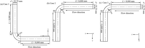
Table 2. Properties in the oil and water phases (Elseth et al., 2001).

Parameter	Value
Oil density (ρo)	790 kg/m^3
Oil viscosity (μo)	0.0016 Pa.s
Water density (ρw)	1000 kg/m^3
Water viscosity (μw)	0.00103 Pa.s
Interfacial tension (σ)	0.043 N/m

2.3.2. Grid information and boundary conditions

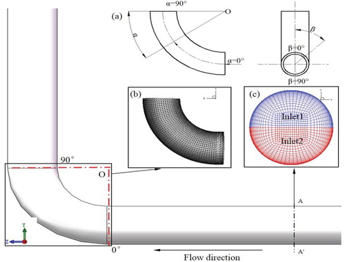
Figure 2 shows a schematic of the grid that was generated for the elbow system. A hexahedral structured grid was adopted, and the elbow part has an encryption treatment as depicted in Figure 2(b). According to the requirements of the wall function, the value of y+ should not be more than 1, as suggested in some studies (Keller, 1978; Rahimzadeh, Maghsoodi, Sarkardeh, & Tavakkol, 2014). Thus, the height of the first layer in the vicinity of the wall was set to 0.1 mm, and the stretching ratio was specified as 1.2. The oil and water phases enter the pipe separately from Inlet1 and Inlet2, for which the mixture velocity is 1.05 m/s and the water volume fraction is 25%. The outlet is set as the pressure outlet, with a value of 0 MPa. The wall is specified as the no-slip boundary condition.

Figure 2. Schematic of the grid for the elbow system: (a) sketch; (b) local encryption treatment; (c) schematic diagram of the inlet mesh generation.

2.3.3. Grid independence and numerical method validation

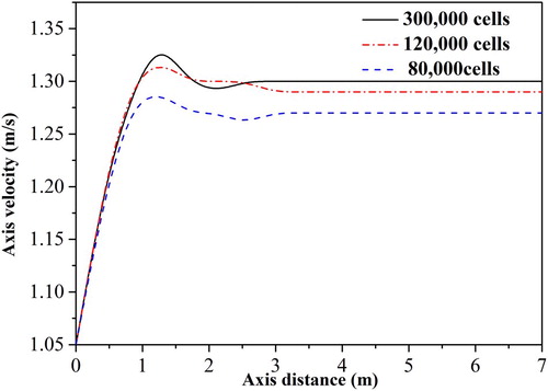
In order to verify the grid independence, the axial velocity distributions along the flow direction of a horizontal pipe were calculated. Three grid numbers of 300,000, 120,000, and 80,000 were adopted for the comparison. It can be seen from Figure 3 that when the grid number reaches about 120,000, the relative error of the curve is less than 0.7% and the variation of the curve becomes stable, thus validating the grid independence. Therefore, a grid number of 120,000 was used for the below calculations.

Figure 3. Comparison of the different grid numbers used to model the horizontal pipe.

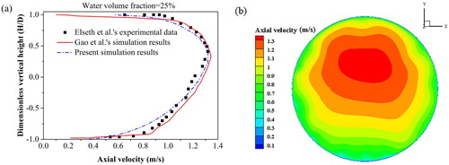
In order to validate the accuracy of the numerical methods, several numerical simulations of the oil–water flow in a horizontal pipe were performed. The properties of the oil and water phases are similar to those in the study by Gao, Gu, and Guo (2003), the detailed parameters for which can be found in Elseth et al. (2001). The mixture velocity is set as 1.05 m/s and the water fraction ranges from 25% to 75%. The results of the water fraction along the normal direction are presented in Figures 4 and 5. It is clear that the present numerical results are a good fit with the experimental data, which indicates that the numerical method is suitable for accurately calculating oil–water two-phase flows. In addition, the numerical results for the axial mean velocity were verified through comparison with the numerical data of Gao et al. (2003) and the experimental data of Elseth et al. (2001), and it can be seen from Figure 6 that the present results are in good agreement with the results of the two studies for the case of $\alpha \text{w}$ = 25%.

Figure 4. Comparison of the present numerical results and the experimental data of Elseth et al. (2001) for the water fraction along the normal direction.

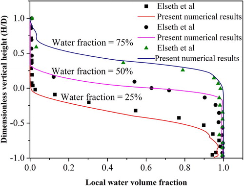
Figure 5. Contours of the water fraction in the cross-section of the pipe: (a) $\alpha \text{w}$ = 25%; (b) $\alpha \text{w}$ = 50%; (c) $\alpha \text{w}$ = 75%.

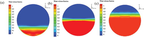
Figure 6. Comparison of the present numerical results, the numerical results of Gao et al. (2003), and the experimental data of Elseth et al. (2001) for the contour of the axial mean velocity when $\alpha \text{w}$ = 25%.

3. Results and discussion

3.1. Distributions of the water phase

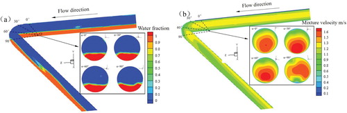
Figure 7 presents the distributions of the water fraction and mixture velocity in Case1. The oil–water two-phase flow is stratified in the horizontal part, and there is little water dispersing into the oil phase, which is in agreement with the flow pattern maps of Kee, Richter, Babic, and Nešić (2016) and Zhang et al. (2019). However, the flow gradually becomes annular in the elbow part under the effect of the centrifugal force. Due to the constraints of the walls, the water layer at the bottom is squeezed by the upper layer of water and flow toward the circular direction. This phenomenon also occurs in U-shape and C-shape tubes (Hu, Ding, Wei, Huang, & Wang, 2010; Jiang, Wang, Ou, & Chen, 2014; Vashisth & Nigam, 2009). The flow is stratified when the direction of the centrifugal force is consistent with the force of gravity; however, when the direction of the centrifugal force is opposed by gravity, the form of the flow pattern changes. The thickness of the water layer in the intrados gradually increases, whereas it decreases in the extrados. It seems that there is no direct water wetting process in the intrados for angles of less than 60°. In addition, for the distributions of the mixture velocity, it appears that the maximum values occur at the intrados of the elbow and the outer wall of the vertical pipe. These maximum velocities both result from the washing of the oil phase, resulting in a lower corrosion risk compared to other locations.

Figure 7. Distributions in Case1 of: (a) the water fraction; (b) the mixture velocity.

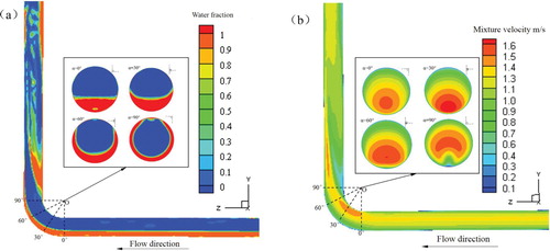
The distributions of the water fraction and mixture velocity in Case2 are illustrated in Figure 8. At the elbow part, the trend of the water phase is to tilt down from the intrados of the elbow. Under the effect of inertia, the water nearly reaches the outer wall of the vertical pipe. The water layer is gradually lifted from the surface with the increment of the angle, and the wetting region also gradually decreases. Compared with Case1, the water in the vertical pipe seldom disperses into the center. The mixture velocity has a relatively stable form and the high-speed region gradually spreads out to the sides, as depicted in Figure 8(b). However, the spreading rate under the effect of the gravity is faster than with Case1. In contrast to Case1, the maximum velocity region is mainly generated by the washing of the water phase.

Figure 8. Distributions in Case2 of: (a) the water fraction; (b) the mixture velocity.

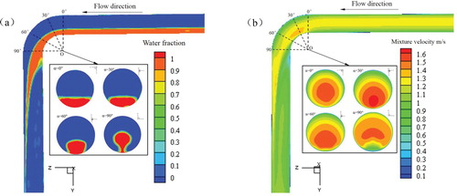
Figure 9 shows the distributions of the water fraction and mixture velocity in Case3. It can be seen that there is a slight change in the water layer thickness when the fluid flows through the elbow part. The mixture velocity takes an asymmetric form; the high-speed region is gradually lifted and gets closer to the intrados of the elbow. Even though water accumulates at the bottom of the pipe for angles greater than 60°, the wall-thinning rate of the pipeline is reduced because of the lower water velocity.

Figure 9. Distributions in Case3 of: (a) the water fraction; (b) the mixture velocity.

3.2. Distributions of the wall shear stress

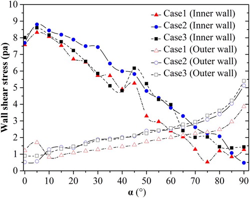
The distributions of the wall shear stress were also investigated in order to further understand the corrosion process (Figures 10 and 11). It can be seen that the maximum wall shear stress for the three cases occurs at the intrados of the elbow, the maximum value located at about 5°. Along the flow direction, the wall shear stress on the intrados of the elbow shows a decreasing trend, whereas the shear stress on the outer wall of the elbow shows a rising trend; the maximum shear stress at the outer wall is located at nearly 90°. These trends are similar to the distributions of the mixture velocity (Figures 7 to 9). Under the effect of gravity, the wall shear stress in Case1 is greatest, while Case2 has the least wall shear stress. It should be noted that in Case2 there is no direct contact between the wall and the water at the location of the maximum wall shear stress – thus, the corrosion risk is lowest in Case2.

Figure 10. Distributions of the wall shear stress for: (a) Case1; (b) Case2; (c) Case3.

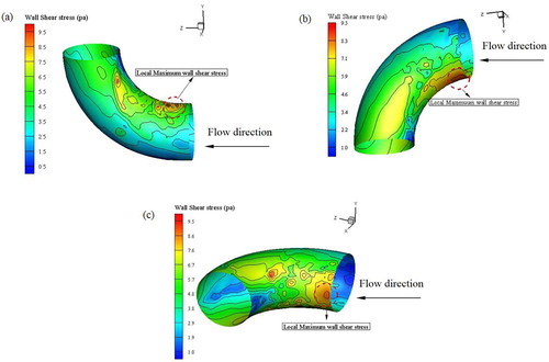
Figure 11. Distributions of the wall shear stress at the inner and outer walls for the three flow configurations.

3.3. Distributions of the mass transfer coefficient

The mass transfer coefficient is an important parameter that is usually adopted to predict the thinning of pipelines due to corrosion. Many scholars have proposed different expressions for the mass transfer coefficient, the basic form for which is: (16) $J=km\left(C_w-C_b\right),$(16) where J is the fluid flux (m³/s), k_m is the mass transfer coefficient (m/s), C_w is the concentration of ferric iron near the wall, and C_b is the concentration of ferric iron in the fully developed flow region. Because the difference between C_w and C_b is small, the mass transfer coefficient is usually utilized to predict the corrosion process. By considering real-world geometric factors and pipeline conditions, Berger and Hau (1977) proposed a formulation for calculating the mass transfer coefficient: (17) $km=\frac{0.0165{Re}^{0.86}{Sc}^{0.33}D}{d},$(17) (18) $Sc=\frac{\upsilon }{D},$(18) (19) $D=\frac{RT{\lambda }_o}{{|Z_o|}^2{F}^{2}C{v}_{+}},$(19) where Re is the Reynolds number, Sc is the Sherwood number, D is the diffusion coefficient (which is shown in Equation (19) and can be obtained from Peng & Zawodzinski, 2018), R is the gas constant, T is the absolute temperature, F is the Faraday constant, λ₀ is the ionic conductivity, C is the cation concentration, Z₀ is the ion valence, and v₊ is the cation number of the charge carrier. In this study, the coefficients C and v₊ are basically set to 1, and the diffusion coefficient of the pipeline is calculated according to the concentration of iron ions: its value is D = 7.12 ×10⁻¹⁰ m²/s (Zheng, He, & Che, 2007).

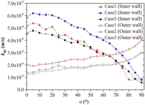
Figure 12 shows the distributions of the mass transfer coefficient for the three flow configurations. It can be seen that the maximum value of the mass transfer coefficient for all three flow directions occurs on the inner wall of the elbow. From the perspective of quantitative analysis, as shown in Figure 13, it can be seen that the maximum mass transfer coefficient is mainly distributed at 5° along the inner wall of the elbow. Along the flow direction, the mass transfer coefficient presents a decreasing trend on the inner wall of the elbow and an increasing trend on the outer wall of the elbow, which is similar to the distributions of the wall shear stress. However, it should be noted that the mass transfer coefficient is based on single-phase flow. For all cases, the calculations of the mass transfer coefficient are not accurate when the oil phase comes into contact with the pipe wall. Only by combining these data with the analysis of the water wetting process can the prediction method be made reliable.

Figure 12. Distributions of the mass transfer coefficient for: (a) Case1; (b) Case2; (c) Case3.

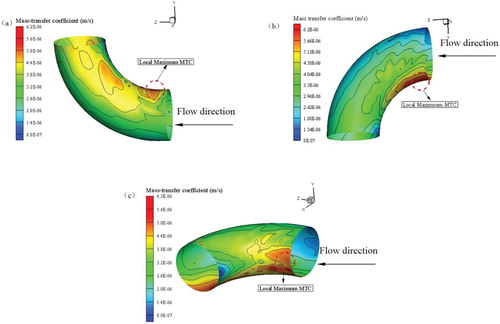
Figure 13. Distributions of the mass transfer coefficient at the inner and outer walls for the three flow configurations.

3.4. Water layer thickness

In long-distance pipelines, stratified flow of the oil–water phase is the most common flow pattern. Figure 14 presents a schematic diagram of the oil–water two-phase flow interface, wherein the water layer thickness $\delta$ is used to represent the wetting process (Barnea, 1987; Zhang et al., 2019): (20) $\delta =\frac{h}{d},$(20) where h is the height of the water layer and d is the diameter of pipe.

Figure 14. Schematic diagram of the oil–water two-phase interface.

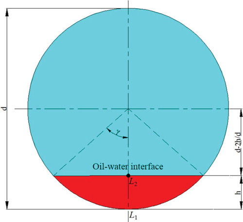
Figure 15 shows the distributions of the water layer thickness along the vertical elbow flow direction for the three flow configurations. It can be seen that the water layer thickness reduces gradually along the flow direction in Case1, and that the perimeter of the water wetting increases gradually. In Case2, due to the effect of gravity, the water layer thickness gradually increases and the area in contact with the water gradually decreases. The water phase gradually radiates from the bottom to the outer wall. Finally, in Case3, the thickness of the water layer in the elbow is relatively stable, which leads to thorough contact with the bottom wall.

Figure 15. Distributions of the water layer thickness for: (a) Case1; (b) Case2; (c) Case3.

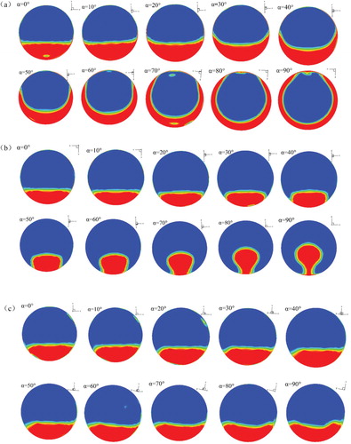
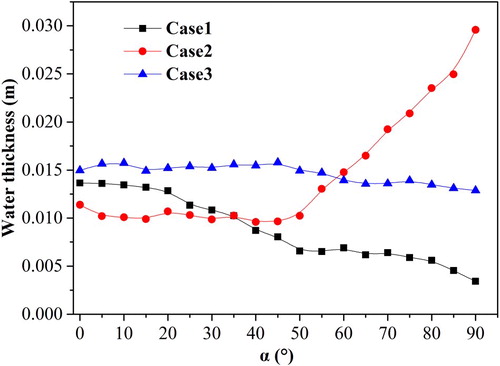
Figure 16 presents the distributions of the water layer thickness at the bottom wall of the elbow for the three flow configurations. It can be seen that when the angle is less than 20° there is little change in the water layer thickness in all three cases. However, in Case1 the water layer thickness decreases gradually, which is similar to the phenomenon shown in Figure 15(a). In Case2, the water layer thickness increases rapidly when the angle is greater than 45°. Thus, when factoring in this analysis of the water layer thickness, it can be seen that the region at high risk of corrosion in Case1 is the extrados of the elbow at an angle of 90°, whereas in Case2 it is the intrados of the elbow wall at an angle of 5°. Lastly, in Case3 the bottom wall of the pipe can be viewed as the region that is at high risk of corrosion.

Figure 16. Distributions of the water layer thickness at the bottom wall of the elbow for the three flow configurations.

3.5. Corrosion mechanism and multiparameter prediction model

The corrosion process can be divided into two parts: the surface chemical reaction process and the reactant/product transportation process. Generally, the reaction rate of the corrosion process is greater than the transportation rate of the reactants/products. Thus, the corrosion rate is mainly determined by the transportation process. In many metals, a protective oxide layer forms at the interface of the metal and the corrosive media, which has a significant effect on the corrosion rate. For the corrosion of metal covered by an oxide layer, the wall shear stress can be used to characterize the process. For the corrosion of metal without an oxide layer, the mass transfer coefficient is usually used to predict the process.

Given the differences between single-phase and two-phase flows, it may not be suitable to use only the wall shear stress and mass transfer coefficient to predict potential corrosion locations in the latter. Even though a number of studies have proved the prediction accuracy of the wall shear stress and mass transfer coefficient through conducting experiments and numerical simulations in the aqueous phase (Ajmal, Arya, & Udupa, 2019; Keshtkar, Nematollahi, & Erfaninia, 2016; Madasamy et al., 2018; Prasad, Gopika, Sridharan, & Parida, 2018), in a multiphase flow system the water wetting process should also be considered. Thus, the present work proposes the use of a multiparameter model to predict corrosion risk, incorporating the wall shear stress, mass transfer coefficient, and water volume fraction. Several studies have demonstrated that factors such as the water cut, velocity, density, interfacial tension, and pipe diameter all affect the intensity of the water wetting and thus influence internal corrosion processes in oil–water two-phase flows. The relationship between the corrosion rate and the type of wetting for oil–water flow at different water cuts has been investigated experimentally (Li, 2009; Tang et al., 2007), with the results showing that the state of the water wetting such as oil wetting, intermittent wetting, and water wetting has a pronounced effect on the corrosion rate. Thus, the multiparameter model proposed in the present study is more suitable for use in real-world configurations. It has been shown in Sections 3.1 to 3.3 that the maximum values of the wall shear stress and mass transfer coefficient under different flow configurations occur at the intrados of the elbow. However, the horizontal-upward elbow flow does not come into contact with the water phase and is thus free of corrosion. The aforementioned phenomena reveal that the maximum values of the wall shear stress and mass transfer coefficient used in conjunction with the water phase is the most efficient method for predicting the locations of regions at high risk of corrosion.

4. Conclusion

In this study, the VOF method and the RNG k-ε model were utilized to simulate the oil–water flow in different elbow configurations. The results were compared to existing data to verify the accuracy of the numerical method, after which the flow characteristics were investigated to analyze the hydrodynamic characteristics related to the corrosion process. The main conclusions are as follows:

1. In all three flow configurations, the maximum wall shear stress and mass transfer coefficient are located on the inner wall of the elbow. However, in horizontal-upward and horizontal-horizontal elbow flow, the maximum values are caused by the washing of the oil phase. The water does not seem to come into direct contact with the wall at these locations, meaning that the corrosion risk in these pipelines is low.

2. In horizontal-downward elbow flow, the maximum wall shear stress and mass transfer coefficient under the condition of the water wetting are located at an angle of about 5° on the inner elbow wall, indicating a higher corrosion risk in this location. For horizontal-upward elbow flow, however, the region at high risk of corrosion is located on the extrados of the elbow at an angle of 90°. For horizontal-horizontal elbow flow, the region at high risk of corrosion is located on the bottom wall of the elbow.

3. The elbow flow forms have a prominent effect on the corrosion locations – however, for horizontal-downward elbow flow, the maximum wall shear stress and mass transfer coefficient in regions at high risk of corrosion are greatest, indicating that the horizontal-downward elbow flow is the layout that is most prone to corrosion.

The corrosion of metal is a complex process which is affected by many factors. This study only addresses the effects of elbow flow direction under stratified flow, and future studies will need to examine a range of different flow patterns in order to more deeply explore this topic. In addition, the diffusion process of products/reactants and the protection offered by metal oxide layers also need to be investigated.

Disclosure statement

No potential conflict of interest was reported by the authors.

Additional information

Funding

This work was supported by the National Natural Science Foundation of China [grant no. 51806198]; and the Scientific Research Foundation of Zhejiang Sci-Tech University [grant no. 18022110-Y].

References

- Ajmal, T. S., Arya, S. B., & Udupa, K. R. (2019). Effect of hydrodynamics on the flow accelerated corrosion (FAC) and electrochemical impedance behavior of line pipe steel for petroleum industry. International Journal of Pressure Vessels and Piping, 174, 42–53. doi: 10.1016/j.ijpvp.2019.05.013
- Barnea, D. (1987). A united model for predicting flow-pattern transition for the whole range of pipe inclinations. International Journal of Multiphase Flow, 13(1), 1–12. doi: 10.1016/0301-9322(87)90002-4
- Berger, F. P., & Hau, K.-F. F.-L. (1977). Mass transfer in tyrbulent pipe flow measured by the electochemical method. International Journal of Heat and Mass Transfer, 20(11), 1185–1194. doi: 10.1016/0017-9310(77)90127-2
- Brackbill, J. U., Kothe, D. B., & Zemach, C. (1992). A Continuum method for modeling surface tension. Journal of Computatiomnal Physics, 100(2), 335–354. doi: 10.1016/0021-9991(92)90240-Y
- Cai, J., & Nesic, S. (2004). Modeling of water wetting in oil–water pipe flow. Corrosion/2004, paper, (04663), 1–19.
- Chen, S., Liu, K., Liu, C., Wang, D., Ba, D., Xie, Y., & Lin, Q. (2016). Effects of surface tension and viscosity on the forming and transferring process of microscale droplets. Applied Surface Science, 388, 196–202. doi: 10.1016/j.apsusc.2016.01.205
- El-Gammal, M., Mazhar, H., Cotton, J. S., Shefski, C., Pietralik, J., & Ching, C. Y. (2010). The hydrodynamic effects of single-phase flow on flow accelerated corrosion in a 90-degree elbow. Nuclear Engineering and Design, 240(6), 1589–1598. doi: 10.1016/j.nucengdes.2009.12.005
- Elseth, G., Kvandal, H., & Melaaen, M. (2001). Measurement of velocity and phase fraction in stratified oil/water flow. Paper presented at the international symposium on Multiphase Flow and Transport Phenomena (ISMFTP), Porsgrunn, Norway.
- Gao, H., Gu, H.-Y., & Guo, L.-J. (2003). Numerical study of stratified oil–water two-phase turbulent flow in a horizontal tube. International Journal of Heat and Mass Transfer, 46(4), 749–754. doi: 10.1016/s0017-9310(02)00321-6
- Hanafizadeh, P., Hojati, A., & Karimi, A. (2015). Experimental investigation of oil–water two phase flow regime in an inclined pipe. Journal of Petroleum Science and Engineering, 136, 12–22. doi: 10.1016/j.petrol.2015.10.031
- Henkes, R. A. W. M., Vlugt, F. F. V. D., & Hoogendoorn, C. J. (1991). Natural-convection flow in a square cavity calculated with low-reynolds-number turbulence models. International Journal of Heal Mass Transfer, 34(2), 337–388. doi: 10.1016/0017-9310(91)90258-G
- Hirt, C. W., & Nichols, B. D. (1981). Volume of fluid (VOF) method for the dynamics of free boundaries. Journal of Computational Physics, 39(1), 201–225. doi: 10.1016/0021-9991(81)90145-5
- Hu, H., & Cheng, Y. F. (2016). Modeling by computational fluid dynamics simulation of pipeline corrosion in CO2-containing oil–water two phase flow. Journal of Petroleum Science and Engineering, 146, 134–141. doi: 10.1016/j.petrol.2016.04.030
- Hu, H., Ding, G., Wei, W., Huang, X., & Wang, Z. (2010). Heat transfer characteristics of refrigerant-oil mixtures flow boiling in a horizontal C-shape curved smooth tube. International Journal of Refrigeration, 33(5), 932–943. doi: 10.1016/j.ijrefrig.2010.02.005
- Issakhov, A., Bulgakov, R., & Zhandaulet, Y. (2018). Numerical simulation of the dynamics of particle motion with different sizes. Engineering Applications of Computational Fluid Mechanics, 13(1), 1–25. doi: 10.1080/19942060.2018.1545253
- Jeong, W., & Seong, J. (2014). Comparison of effects on technical variances of computational fluid dynamics (CFD) software based on finite element and finite volume methods. International Journal of Mechanical Sciences, 78, 19–26. doi: 10.1016/j.ijmecsci.2013.10.017
- Jiang, F., Wang, Y., Ou, J., & Chen, C. (2014). Numerical simulation of oil–water core annular flow in a U-bend based on the Eulerian model. Chemical Engineering & Technology, 37(4), 659–666. doi: 10.1002/ceat.201300809
- Kee, K. E., Richter, S., Babic, M., & Nešić, S. (2016). Experimental study of oil–water flow patterns in a large diameter flow loop-the effects on water wetting and corrosion. Corrosion, 72(4), 569–582. doi: 10.5006/1753
- Keller, H. B. (1978). Numerical methods in boundary-layer theory. Annual Review of Fluid Mechanics, 10(1), 417–433. doi: 10.1146/annurev.fl.10.010178.002221
- Kermani, M. B., & Morshed, A. (2003). Carbon Dioxide corrosion in oil and gas production-a compendium. Critical Review of Corrosion Science and Engineering, 59(8), 859–683. doi: 10.5006/1.3277596
- Keshtkar, K., Nematollahi, M., & Erfaninia, A. (2016). CFX study of flow accelerated corrosion via mass transfer coefficient calculation in a double elbow. International Journal of Hydrogen Energy, 41(17), 7036–7046. doi: 10.1016/j.ijhydene.2016.02.072
- Li, C. (2009). Effect of corrosion inhibitor on water wetting and carbon dioxide corrosion in oil–water two-phase flow (Doctoral dissertation, PhD dissertation). Russ College of Engineering and Technology, Ohio State University.
- Lin, C. H., & Ferng, Y. M. (2014). Predictions of hydrodynamic characteristics and corrosion rates using CFD in the piping systems of pressurized-water reactor power plant. Annals of Nuclear Energy, 65, 214–222. doi: 10.1016/j.anucene.2013.11.007
- Madasamy, P., Krishna Mohan, T. V., Sylvanus, A., Natarajan, E., Rani, H. P., & Velmurugan, S. (2018). Hydrodynamic effects on flow accelerated corrosion at 120°C and neutral pH conditions. Engineering Failure Analysis, 94, 458–468. doi: 10.1016/j.engfailanal.2018.08.021
- Magnini, M., Ullmann, A., Brauner, N., & Thome, J. R. (2018). Numerical study of water displacement from the elbow of an inclined oil pipeline. Journal of Petroleum Science and Engineering, 166, 1000–1017. doi: 10.1016/j.petrol.2018.03.067
- Menad, N. A., Noureddine, Z., Hemmati-Sarapardeh, A., Shamshirband, S., Mosavi, A., & Chau, K.-w. (2019). Modeling temperature dependency of oil–water relative permeability in thermal enhanced oil recovery processes using group method of data handling and gene expression programming. Engineering Applications of Computational Fluid Mechanics, 13(1), 724–743. doi: 10.1080/19942060.2019.1639549
- Nešić, S. (2007). Key issues related to modelling of internal corrosion of oil and gas pipelines – A review. Corrosion Science, 49(12), 4308–4338. doi: 10.1016/j.corsci.2007.06.006
- Peng, J., & Zawodzinski, A. T. (2018). Ion transport in phase-separated single ion conductors. Journal of Membrane Science, 555, 38–44. doi: 10.1016/j.memsci.2018.03.029
- Pietralik, J. M., & Schefski, C. S. (2009). Flow and mass transfer in bends under flow accelerated corrosion wall thinning conditions. Presented at the 17th international conference on Nuclear Engineering, ICNE, Brussels, Belgium.
- Pietralik, J. M., & Smith, B. A. W. (2006). CFD applications to flow accelerated corrosion in feeder bends. Presented at the 14th international conference on Nuclear Engineering, Miami, FL. doi:10.1115/ICONE17-75416
- Pouraria, H., Seo, J. K., & Paik, J. K. (2016a). Numerical modelling of two-phase oil–water flow patterns in a subsea pipeline. Ocean Engineering, 115, 135–148. doi: 10.1016/j.oceaneng.2016.02.007
- Pouraria, H., Seo, J. K., & Paik, J. K. (2016b). A numerical study on water wetting associated with the internal corrosion of oil pipelines. Ocean Engineering, 122, 105–117. doi: 10.1016/j.oceaneng.2016.06.022
- Prasad, M., Gopika, V., Sridharan, A., & Parida, S. (2018). Pipe wall thickness prediction with CFD based mass transfer coefficient and degradation feedback for flow accelerated corrosion. Progress in Nuclear Energy, 107, 205–214. doi: 10.1016/j.pnucene.2018.04.024
- Rahimzadeh, H., Maghsoodi, R., Sarkardeh, H., & Tavakkol, S. (2014). Simulating flow over circular spillways by using different turbulence models. Engineering Applications of Computational Fluid Mechanics, 6(1), 100–109. doi: 10.1080/19942060.2012.11015406
- Rani, H. P., Divya, T., Sahaya, R. R., Kain, V., & Barua, D. K. (2014). CFD study of flow accelerated corrosion in 3D elbows. Annals of Nuclear Energy, 69, 344–351. doi: 10.1016/j.anucene.2014.01.031
- Shi, J., Gourma, M., & Yeung, H. (2017). CFD simulation of horizontal oil–water flow with matched density and medium viscosity ratio in different flow regimes. Journal of Petroleum Science and Engineering, 151, 373–383. doi: 10.1016/j.petrol.2017.01.022
- Song, X., Yang, Y., Zhang, T., Xiong, K., & Wang, Z. (2017). Studies on water carrying of diesel oil in upward inclined pipes with different inclination angle. Journal of Petroleum Science and Engineering, 157, 780–792. doi: 10.1016/j.petrol.2017.07.076
- Sun, H. T., Sze, K. Y., Tang, A. Y. S., Tsang, A. C. O., Yu, A. C. H., & Chow, K. W. (2019). Effects of aspect ratio, wall thickness and hypertension in the patient-specific computational modeling of cerebral aneurysms using fluid-structure interaction analysis. Engineering Applications of Computational Fluid Mechanics, 13(1), 229–244. doi: 10.1080/19942060.2019.1572540
- Tang, P., Yang, J., Zheng, J., & Wong, I. (2009). Failure analysis and prediction of pipes due to the interaction between multiphase flow and structure. Engineering Failure Analysis, 16(5), 1749–1756. doi: 10.1016/j.engfailanal.2009.01.002
- Tang, X., Li, C., Ayello, F., Cai, J., Nesic, S., Cruz, C. I. T., & AL-Khamis, J. N. (2007). Effects of oil type on phase wetting transition and corrosion in oil–water flow (NACE Paper No. 07170).
- Tang, X., Richter, S., & Nesic, S. (2008). Study of wettability of different mild surface. Presented at the 17th International Corrosion Congress, Athens.
- Utanohara, Y., & Murase, M. (2019). Influence of flow velocity and temperature on flow accelerated corrosion rate at an elbow pipe. Nuclear Engineering and Design, 342, 20–28. doi: 10.1016/j.nucengdes.2018.11.022
- Vashisth, S., & Nigam, K. D. P. (2009). Prediction of flow profiles and interfacial phenomena for two-phase flow in coiled tubes. Chemical Engineering and Processing: Process Intensification, 48(1), 452–463. doi: 10.1016/j.cep.2008.06.006
- Xu, X.-X. (2007). Study on oil–water two-phase flow in horizontal pipelines. Journal of Petroleum Science and Engineering, 59(1–2), 43–58. doi: 10.1016/j.petrol.2007.03.002
- Yang, J., Teng, P., & Zhang, H. (2018). Experiments and CFD modeling of high-velocity two-phase flows in a large chute aerator facility. Engineering Applications of Computational Fluid Mechanics, 13(1), 48–66. doi: 10.1080/19942060.2018.1552201
- Zhang, G. A., Zeng, L., Huang, H. L., & Guo, X. P. (2013). A study of flow accelerated corrosion at elbow of carbon steel pipeline by array electrode and computational fluid dynamics simulation. Corrosion Science, 77, 334–341. doi: 10.1016/j.Corsci.2013.08.022
- Zhang, H., Lan, H.-q., & Lin, N. (2019). A numerical simulation of water distribution associated with internal corrosion induced by water wetting in upward inclined oil pipes. Journal of Petroleum Science and Engineering, 173, 351–361. doi: 10.1016/j.petrol.2018.10.030
- Zhang, J., Wang, Z. L., Wang, Z. M., & Han, X. (2012). Chemical analysis of the initial corrosion layer on pipeline steels in simulated CO2-enhanced oil recovery brines. Corrosion Science, 65, 397–404. doi: 10.1016/j.corsci.2012.08.045
- Zheng, D., & Che, D. (2006). Experimental study on hydrodynamic characteristics of upward gas–liquid slug flow. International Journal of Multiphase Flow, 32(10–11), 1191–1218. doi: 10.1016/j.ijmultiphaseflow.2006.05.012
- Zheng, D., He, X., & Che, D. (2007). CFD simulations of hydrodynamic characteristics in a gas–liquid vertical upward slug flow. International Journal of Heat and Mass Transfer, 50(21–22), 4151–4165. doi: 10.1016/j.ijheatmasstransfer.2007.02.041