Modeling natural gas compressibility factor using a hybrid group method of data handling

Abstract

The natural gas compressibility factor indicates the compression and expansion characteristics of natural gas under different conditions. In this study, a simple second-order polynomial method based on the group method of data handling (GMDH) is presented to determine this critical parameter for different natural gases at different conditions, using corresponding state principles. The accuracy of the proposed method is evaluated through graphical and statistical analyses. The method shows promising results considering the accurate estimation of natural gas compressibility. The evaluation reports 2.88% of average absolute relative error, a regression coefficient of 0.92, and a root means square error of 0.03. Furthermore, the equations of state (EOSs) and correlations are used for comparative analysis of the performance. The precision of the results demonstrates the model’s superiority over all other correlations and EOSs. The proposed model can be used in simulators to estimate natural gas compressibility accurately with a simple mathematical equation. This model outperforms all previously published correlations and EOSs in terms of accuracy and simplicity.

KEYWORDS:

• Group method of data handling (GMDH)
• natural gas compressibility factor
• big data
• correlation
• equations of state (EOSs)
• data-driven model
• artificial intelligence (AI)

1. Introduction

The increasing demand for oil and coal as energy and the technological and environmental concerns associated with its production and consumption have drawn attention toward natural gas. The natural gas consumption generates fewer pollutants and greenhouse gases (Kamari, Hemmati-Sarapardeh, Mirabbasi, Nikookar, & Mohammadi, 2013; Shateri, Ghorbani, Hemmati-Sarapardeh, & Mohammadi, 2015). Critical insight into the behavior of natural gas is important to the reservoir and the chemical engineering calculations that deal with gas as one of the main phases. Among the parameters of evaluating the behavior of natural gas, the compressibility is of utmost importance in determining the natural gas phase behavior. Gas compressibility (Z-factor) represents the proportion of volume a given amount of gas to the ideal volume of it at the common conditions and defined pressure and temperature. Gas compressibility makes the difference between ideal gas and real gas. The following relationship is generally used to calculate gas compressibility (McCain, 2017): (1) $Z=\frac{V_{real}}{V_{ideal}}=\frac{V}{(nRT)/P}$(1) Where V_real (V) and V_ideal denote the real and ideal gas volumes, respectively. Furthermore, R and z represent the universal gas constant, and the gas compressibility factor, respectively. T, P, and n represent the gas temperature, pressure, and some moles, respectively.

At low pressure and temperature conditions, gas molecules have fewer interactions and collisions, and behavior can be considered ideal. However, at a higher pressure or temperature, the collision and interaction of the molecules increase. This phenomena has to be taken into account when making predictions for gas expansion or contraction (Firoozabadi, 1999; Shateri et al., 2015).

There are various techniques to measure the compressibility factor. One main way is by performing compression-expansion experiments. Overall, the experimental measurement of the compressibility factor appeared to be an accurate approach compared to all other approaches. However, they are generally slow, cumbersome, and costly. Also, it is reported not feasible to conduct an experiment for every single condition considering various pressure and temperature at which the compressibility is needed. Using equations of state (EOS) is another approach to determine the compressibility factor. When utilizing EOS, the reservoir characteristics are being employed. Generally, these equations come from the following form when the gas compressibility factor is the target PVT parameter (McCain, 2017): (2) $Z^3+a\times Z^2+b\times Z+c=0$(2) where a, b, and c donate the empirical constants of composition functions for temperature, pressure, and gas. Furthermore, Z denotes the gas compressibility factor. Even though these equations are advantages and their implementation can facilitate the measurement of other gas properties such as enthalpy, entropy, and Gibbs free energy, they are usually implicit higher-order equations that require intense computations. Besides the complex computations, the binary interaction coefficients used in some EOS’s need to be measured by conducting experiments that may not be practical. Further, it has been shown that these equations are not suitable for predicting hydrocarbon gas properties (Elsharkawy, 2004).

Empirical correlations are another source of determining gas compressibility factor, which is easy and fast to use but is generally associated with erroneous predictions (Kamyab, Sampaio, Qanbari, & Eustes, 2010; Kumar, 2004; Sanjari & Lay, 2012b). A minor estimation error in the compressibility factor of correlations would lead to a false prediction of formation, density and the amount of gas. Therefore, the development of fast, user-friendly, and accurate models to predict the compressibility factor is critical.

Several researchers have attempted to develop methods to estimate the compressibility factor. For instance, Standing and Katz (1942) advanced a graphical technique based on pseudo-reduced. Van Der Waals and Rowlinson (2004) was one of the pioneers of EOS methods by taking into account the intramolecular forces and volume of molecules. Using Van der Waals EOS for determining gas compressibility factor leads to higher accuracy compared to the empirical approach introduced by Katz and Standing. There is a number of researches contributed to the development of reliable EOS’s (Soave, 1972).

A general expression for the PVT relationship of fluids has the following form (Shateri et al., 2015): (3) $P=\frac{RT}{V-b}=\frac{a}{v^2-uv-w^2}$(3) An expression for gas compressibility factor can be written by rewriting the above equation and implementing the equation for gas compressibility factor as follows: (4) $\begin{array}{rl}& Z^3-(1+B-U)Z^2+(A-BU-U-W^2)Z\\ & -(AB-B{W}^2-W^2)=0\end{array}$(4) Where A, B U, and W are dimensionless parameters that are extracted from the current temperature, composition, and pressure.

For the purpose of advancing more efficient, yet faster methods, adequate researchers have developed correlations that can be explicitly used to address the problem. In 1973, Hall and Yarborough (1973) transformed the graphical chart of Katz and Standing into a relatively simple correlation by fitting their correlation to the chart and determining the correlation coefficients. Beggs and Brill (1973) also employed Katz and Standing chart and developed a correlation to estimate the gas compressibility factor. Dranchuk, Purvis, and Robinson (1973) used an EOS developed by Benedict–Webb–Rubin (Simon & Briggs, 1964) and proposed a gas compressibility correlation in 1974. Abu-Kassem joined Dranchuk in 1975 to develop an analytical equation to decrease the gas density which had been utilized to calculate the gas compressibility factor (Dranchuk & Abou-Kassem, 1975). In 1975, Gopal collected multiple correlations for the gas compressibility factor at various conditions (Gopal, 1977a). Kumar (2004) introduced a novel model for gas compressibility factor to be used by Shell. In 2010, Heidaryan et al. used multiple regression analysis (Heidaryan, Moghadasi, & Rahimi, 2010), and in the same year, Azizi employed genetic programming (Azizi, Behbahani, & Isazadeh, 2010). A comprehensive study of the mentioned methods was conducted by Sanjari and Lay (2012a) in which the performance of the methods mentioned above has been investigated.

The application of artificial intelligence and soft computing for building intelligent methods in many industries has recently attracted much attention (Anitescu, Atroshchenko, Alajlan, & Rabczuk, 2019; Chuntian & Chau, 2002; Fotovatikhah et al., 2018; Guo, Zhuang, & Rabczuk, 2019; Moazenzadeh, Mohammadi, Shamshirband, & Chau, 2018; Taherei Ghazvinei et al., 2018; Yaseen, Sulaiman, Deo, & Chau, 2019). In petroleum and gas industries, intelligent models have been used to determine, oil and gas thermodynamic properties, reservoir formation properties and miscibility conditions required for gas injection processes (Dargahi-Zarandi, Hemmati-Sarapardeh, Hajirezaie, Dabir, & Atashrouz, 2017; Dashtian, Bakhshian, Hajirezaie, Nicot, & Hosseini, 2019; Hajirezaie, Hemmati, & Ayatollahi, 2014; Hajirezaie, Hemmati-Sarapardeh, Mohammadi, Pournik, & Kamari, 2015; Hajirezaie, Pajouhandeh, Hemmati-Sarapardeh, Pournik, & Dabir, 2017; Hajirezaie, Wu, Soltanian, & Sakha, 2019; Hemmati-Sarapardeh, Tashakkori, Hosseinzadeh, Mozafari, & Hajirezaie, 2016; Kamari, Pournik, Rostami, Amirlatifi, & Mohammadi, 2017; Kamari, Safiri, & Mohammadi, 2015; Rostami, Kamari, Panacharoensawad, & Hashemi, 2018). These models take both input and output values to get trained and later can make predictions. Even though the original, intelligent models were considered black-box models, there have been numerous modifications to these models to make them transparent and usable methods, and their performance has significantly improved over the past few years. Intelligent models have been used in many reservoir engineering calculations. There are also some intelligent models that were developed specifically for predicting natural gas properties (Dargahi-Zarandi et al., 2017; Hajirezaie et al., 2015, 2017). We have already developed two intelligent models for predicting natural gas compressibility factor using the same data bank (Kamari et al., 2013; Shateri et al., 2015). However, they are a black box, and their usage generally needs software. Literature still suffers from the lack of a comprehensive, accurate, and simple model for natural gas compressibility estimation.

In this study, a novel supervised approach, namely the group method of data handling (GMDH) was proposed as a robust model to predict the compressibility factor. To do this, a comprehensive data bank of compressibility factor was used considering a diverse range of pressure, temperature, and composition. Several statistical quality measures and graphical methods were utilized to calculate the model performance. Furthermore, for the evaluation of the proposed graphical and the statistical methods, the root mean square error (RMSE), average absolute percent error (AAPRE), regression coefficient (R²), average percentage relative error (APRE), cross-plot, and error distribution curves have been used. Additionally, the performance of previously published well-known correlations and EOSs was investigated and compared to the proposed model.

2. Data acquisition

The reliability of any intelligent model is dependent on the data bank that has been utilized for the purpose of model training and testing. Here, various range of pressure, temperature, and gas composition conditions were used to ensure the development of a valid model that can determine the gas compressibility factor. Two dimensionless parameters of pseudo-reduced for temperature and pressure are studied to be used in the developed model for predicting gas compressibility. These parameters are calculated from the current pressure and temperature, as well as the pseudo critical pressure and temperature calculated as follows: (5) $\begin{array}{l}{p}_{pr}=\frac{P}{p_{pc}}\\ T_{pr}=\frac{T}{T_{pc}}\end{array}$(5) where T_pc and P_pc provide the values of pseudo critical temperature and pressure, respectively. Furthermore, P_pr and T_pr are pseudo-reduced pressure and temperature.

For gas with multiple components, P_pc and T_pc are calculated from the critical temperature and pressure of the individual components as follows: (6) $P_{pc}=\sum _{i=1}^n{y}_i{P}_{ci}$(6) (7) $T_{pc}=\sum _{i=1}^n{y}_i{T}_{ci}$(7) In these equations, T_ci and P_ci provide the values for the critical temperature and pressure of component i. Also, y_i describe the mole fraction of component i.

The data sets in this article gathered from the previously published research and the online repositories, e.g. (Elsharkawy & Foda, 1998; McLeod, 1968; Robinson & Jacoby, 1965; Simon & Briggs, 1964; Whitson & Torp, 1981; Wichert & Aziz, 1972). These data were also used in our previous publications (Kamari et al., 2013; Shateri et al., 2015). Further, Table 1 represents the statistical details of the data bank used. As the table demonstrates, the pressures, temperatures, and compositions comprise a comprehensive range, ensuring that the developed model based on this data set would be a reliable predictor for various types of natural gases at different conditions. Nine hundred seventy-eight data points were used in this study. Eighty percent of the data was used for training and model development and the remained 20% was used to check model performance and validity. The data were divided into training and testing sets randomly.

Table 1. The statistical parameters for the data used for z-factor modeling.

Property	Max.	Min.	Average
C1	97.48	17.27	71.18
C2	28.67	0	3.86
C3	13.16	0	1.44
i-C4	2.23	0	0.21
n-C4	3.10	0	0.36
i-C5	2.85	0	0.18
n-C5	0.79	0	0.10
C6	2.68	0	0.20
C7+	8.17	0	0.64
MwC7+	150	0	50
Sgc7+	0.90	0	0.31
H2S	73.85	0	13.92
CO2	54.46	0	6.00
N2	25.15	0	1.83
Pressure, psi	7026	154	2820
Reservoir temperature, °F	300	40	147
Tpr	1.96	0.97	1.46
Ppr	10.19	0.17	3.75
Z-factor	1.241	0.40	0.86

3. Evaluating the model performance

There are multiple statistical parameters that are employed to assess the performance of a model. The parameters that were used in this work include APRE, AAPRE, RMSE, and R². A simple presentation of the mentioned parameters is presented here:

1. APRE (E_r%): (8) $E_r=\frac{1}{n}\sum _{i=1}^n{E}_i$(8) where E_i stands for the relative variation of predicted value from an experimental value expressed as Percentage Relative Error: (9) $E_i=\left[\frac{{(O)}_{\exp }-{(O)}_{\text{rep}\text{./pred }}}{O_{\exp }}\right]\times 100\Rightarrow i=1,2,3,\dots ,n$(9) 2. AAPRE: (10) $E_a=\frac{1}{n}\sum _{i=1}^n|E_i|$(10) 3. RMSE: (11) $RMSE=\sqrt{\frac{1}{n}\sum _{i=1}^n{({O_i}_{\exp }-{O_i}_{\text{rep}\text{./pred }})}^2}$(11) 4. R²: (12) $R^2=1-\frac{{\sum }_{i=1}^n{(O_{i\exp }-O_{\text{i rep}\text{./pred }})}^2}{{\sum }_{i=1}^n{(O_{\text{i rep}\text{./pred }}-\overline{O})}^2}$(12) In these formulas, $\overline{O}$ is the mean value of experimental data output.

Another approach to evaluate the performance of a model and compare it with other models is the usage of graphical error analysis. The graphical approaches used in this study are cross-plot, frequency vs. absolute relative error, error distribution, and trend analysis curves. Cross-plots are utilized to assess the performance of a model in which the estimated data by the model are plotted against the experimental values, and one can observe the accuracy of the model depending on how close the trend is to a unit-slope line that crosses the origin. Further, the cumulative frequency of data points against the absolute relative error is plotted to quantify the number of data points that can be accurately predicted by the model. Besides, the error distribution curve was investigated to identify the error trend of the model when an independent variable is increased. The proximity of data points to the zero-error line tests the precision of that model. Finally, a trend analysis is performed to investigate whether or not the developed model can accurately estimate the trend of gas compressibility factor at different pressures.

4. Model development

GMDH, every two independent parameters are coupled with a quadratic polynomial expression and form $\left(\begin{array}{c}\mathbf{M}\\ 2\end{array}\right)$ new variables as follows: (14) $Z_i^{GMDH}=a{x}_i+b{x}_j+c{x}_i{x}_j+d{x}_i^2+e{x}_j^2+f$(14) And the new matrix can be represented by the new variables as follows: (15) $v_z=(z_1,z_2,\dots z_n)$(15) In the next step, the least square method is utilized to reduce the difference between the actual data and the model predictions as presented below: (16) ${\delta }_j^2=\sum _{i=1}^{Nt}(y_i-Z_i^{GMDH}{)}^{2}j=1,2\dots ,\left(\begin{array}{c}M\\ 2\end{array}\right)$(16) In this equation, the quantity of data points in the training set is shown by Nt. In the next step, the general matrix is written as follows: (17) $Y=A^{T}X$(17) Writing the general matrix in the above form helps with offering a general formulation to determine the unknown quadratic polynomial coefficients as shown below: (18) $A^T=Y{X}^T(X{X}^T{)}^{-1}$(18) In the later stage, the data set is divided into subsets of testing and training, the model coefficients are obtained during the training stage, and the testing set is utilized to determine the best combination of the two independent variables based on the following condition: (19) ${\delta }_j^2=\sum _{i=Nt+1}^N(y_i-Z_i^{GMDH}{)}^2<\epsilon j=1,2\dots ,\left(\begin{array}{c}M\\ 2\end{array}\right)$(19) The combined variables will be stored if this criterion is met, otherwise the algorithm eliminates this combination of two variables and the iteration will continue. More information about this modeling approach can be found in our previous work (Hemmati-Sarapardeh & Mohagheghian, 2017). This method was recently used for modeling gas compressibility factor of Iranian gas reservoirs (Shariaty, Khorsand Movaghar, & Vatandoost, 2019).

5. Results and discussion

The GMDH has been successfully implemented as an evolutionary intelligent model to predict the natural gas’s compressibility. The inputs of the model were gas composition, pressure, and temperature, as shown in Table 1. In addition to C₁–C₆ and C₇₊ components, H₂S, CO_2, and N₂ gases were considered as the components. The pressure and temperature values are utilized to estimate the pseudo-reduced pressure and temperature as discussed previously. During the data acquisition stage, a wide range of input parameters was considered as shown in Table 1. The pressure ranges from 154 to 7026 Psia, reservoir temperature ranges from 40 to 300°F, and the compressibility factor values cover a wide range of 0.4–1.24. The distribution of input and output data is illustrated in Figure 1. In addition to the data distribution, normal distribution curves were plotted in this figure. Pseudo reduced pressure and temperature were the chosen parameters for this figure due to their impact on any reservoir fluid properties. As can be seen, all three data sets follow a relatively normal shape, especially the gas compressibility factor data. The mean values for the pseudo-reduced temperature, pseudo-reduced pressure, and gas compressibility factor are 1.5, 3.9 and 0.9, respectively. The bin size in all cases is 40. The model’s schematic flowchart is illustrated in Figure 2. In order to assess the accuracy of the developed model, various statistical and graphical methods such as average absolute relative error and error distribution curve were employed as will be discussed in this section.

Figure 1. Distribution of the input and output data sets.

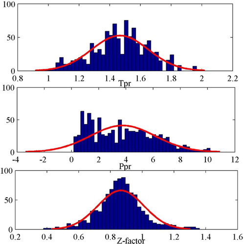
Figure 2. A schematic flowchart of the proposed GMDH for predicting z-factor.

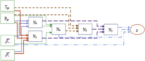
After optimizing the model, the genome and nodal expressions were obtained as follows: (20) $\begin{array}{rl}z& =-0.268213-1.09959N_2\sqrt{T_{pr}}+0.434222T_{pr}^2\\ & -1.02209N_4+0.397836N_4^2+2.58207N_2\end{array}$(20) (21) $\begin{array}{rl}{N}_6& =2.28818+1.46235P_{pr}-1.05874P_{pr}\sqrt{T_{pr}}\\ & +3.50204\sqrt{T_{pr}{P}_{pr}}-0.667833T_{pr}-4.84879\sqrt{P_{pr}}\end{array}$(21) (22) $\begin{array}{rl}{N}_5& =1.88105-0.466011T_{pr}{P}_{pr}+1.5661T_{pr}\sqrt{P_{pr}}\\ & -0.265557T_{pr}^2+0.863307P_{pr}-2.90311\sqrt{P_{pr}}\end{array}$(22) (23) $\begin{array}{rl}{N}_4& =-2.14451-0.0929261P_{pr}{N}_6+0.0120013P_{pr}^2\\ & -4.51872N_6\sqrt{T_{pr}}+1.89131T_{pr}+5.85344N_6\end{array}$(23) (24) $\begin{array}{rl}{N}_3& =-0.461086+0.0344126T_{pr}^2-0.048752P_{pr}\\ & +0.00674994P_{pr}^2+2.4872N_4-1.11543N_4^2\end{array}$(24) (25) $\begin{array}{rl}{N}_2& =-0.182453-17.0122N_5+18.4918N_5{N}_3\\ & +17.1725N_6-18.6856N_6{N}_3+1.22045N_3\end{array}$(25) where T_pr and P_pr represent the pseudo-reduced temperature and pressure, respectively, and N₂–N₆ represents the virtual variables or nodes of the model. Here, the equations are second-order polynomials that are utilized to predict the gas compressibility factor. Considering the first equation, the gas compressibility factor will be estimated through realization of the pseudo- reduced temperature, and the virtual parameters N₂ and N₄ and. N₄ can be calculated by knowing pseudo-reduced pressure and by calculating the virtual parameter N₆. N₆ is a simple function of temperature and pseudo-reduced pressure and can be directly calculated. In order to calculate N₂, the virtual parameters N₃ and N₅ are needed in addition to N₆. N₃ can be calculated after calculating the virtual parameter N₄. Finally, N₅ is directly calculated similarly to N₆ by having pseudo-reduced pressure and temperature. The graphical techniques and statistical quality measures were applied to evaluate the accuracy of the developed model. Furthermore, EOSs are used for further evaluation and comparison. Five EOSs are considered, i.e. Van der Waals, Threfall, Adair, and Roth (1873), Lawal-Lake-Silberberg (Lawal, 1999), Peng and Robinson (1976), Soave-Redlich-Kwong (Soave, 1972), and Patel and Teja (1982). The empirical correlations include Dranchuk, Purvis, and Robinson (1974), Dranchuk and Abou-Kassem (1975), Brill and Beggs (1973), Shell Oil Company (Kumar, 2004), Gopal (1977b), Hall and Yarborough (1973), Sanjari and Lay (2012a), Heidaryan et al. (2010), Azizi et al. (2010), and Kamari, Gharagheizi, Mohammadi, and Ramjugernath (2016). The list of the outcomes of a statistical assessment of the GMDH model and the previously published correlations and EOSs are available in Table 2. Evidently, in this table, the proposed model demonstrates the most accurate performance compared to other models when comparing the RMSE, the average absolute percentage relative error, and the regression coefficient. The Hall Yarborough correlation was found to be the next most accurate model followed by the Patel-Teja EOS model based on the statistical information presented in this table.

Noticing the APRE and AAPRE values of the models in this study reveals that, while the APRE value of some of the models is not smaller than those of others, their AAPRE is. The definition of APRE can be used to explain this observation. As a matter of fact, APRE cannot be used by itself to approve or reject a model. For instance, an APRE value close to zero would be obtained if half of the data points are overestimated by a model and the remaining half are underestimated, which would in return present a false assessment of the model performance. However, if some data points are estimated accurately by a model and the remaining few data points are either underestimated or overestimated, a positive or negative APRE value would be obtained, respectively, which again cannot testify the model performance. As an example, the Van der Waals's model has a much smaller APRE value than that of Dranchuk-Purvis-Robinson. However, it is considered to be a less accurate model than the latter one.

Table 2. Statistical error analyses for the correlations, EOSs, and the GMDH model.

Method	AARE %	RMSE	R^2	AAPRE %
Dranchuk-Abou-Kassem Correlation	4.21	0.0992	0.5748	8.18
Kamari et al.	−1.10	0.0629	0.8248	5.92
Dranchuk-Purvis-Robinson Correlation	4.66	0.0555	0.9064	4.77
Hall-Yarborough Correlation	1.46	0.0429	0.8924	3.59
Beggs-Brill Correlation	4.08	0.0785	0.7763	6.53
Shell Oil Company Correlation	4.36	0.0596	0.7819	6.24
Gopal Correlation	6.12	0.0910	0.7371	6.26
Azizi et al. Correlation	4.26	0.0792	0.7723	6.25
Heidaryan et al. Correlation	3.61	0.0762	0.7788	5.80
Sanjari and Lay Correlation	0.66	0.0697	0.8119	5.67
van der-Waals EOS	0.31	0.0696	0.7711	6.42
Peng-Robinson EOS	−5.34	0.0599	0.8916	6.10
Patel-Teja EOS	−1.18	0.0447	0.8806	4.15
Soave-Redlich-Kwong EOS	−3.14	0.0493	0.8938	4.82
Lawal-Lake-Silberberg EOS	−2.66	0.0453	0.8942	4.43
The GMDH model, Train	−0.21	0.0351	0.9177	2.89
The GMDH model, Test	−0.10	0.0340	0.9171	2.85
The GMDH model, Total	−0.19	0.0349	0.9176	2.88

Another way to illustrate the performance of the models and to compare them more comprehensively is by using graphical analyses. The performance evaluation is done through several graphical analyses considering a number of most popular models from both quantity and quality standpoints. Figure 3 presents the cross-plot of the developed model in which the calculated data is plotted against the measured data for both testing and training sets. The location of the majority of the data points on the y = x line provides the precise predictions of the developed GMDH model for the training and testing phases. The error distribution of the model is shown in Figure 4. As the figure shows, most of the data points are near the zero percent error line. Therefore, as the gas compressibility factor increases, the GMDH model shows no systematic error trend. Worth mentioning that most of the previously published models suffer from an error trend. The figure indicates that the error of the testing set is smaller than the training set. The distribution of the relative error of predictions is plotted in Figure 5. In addition to the distribution of data points, the normal distribution is plotted indicated by the red line. The figure indicates that a Weibull or lognormal distribution may better describe this distribution and that most of the data points (predictions) have a relative error close to zero demonstrating the accuracy of the model in predicting gas compressibility factors. Figures 6 and 7 depict the statistical information reported in Table 2 for a graphical demonstration of the performance of the models. Further, these figures indicate that models with a smaller RMSE do not necessarily have a smaller average absolute percent relative error. This means that when performing statistical analyses, care should be taken to avoid the misinterpretation of the results by focusing on only one statistical parameter.

Figure 3. Cross-plot of the predicted z-factors versus experimental data.

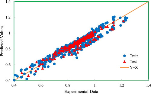
Figure 4. Error distribution curve of the proposed GMDH model versus experimental z-factor.

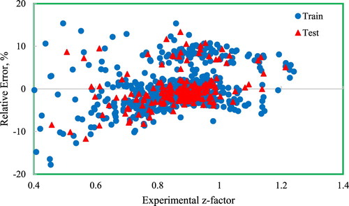
Figure 5. Distribution of relative error of the proposed GMDH model.

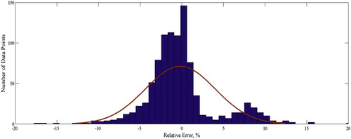
Figure 6. RMSE of the existing correlations, EOSs, and GMDH models for predicting z-factor.

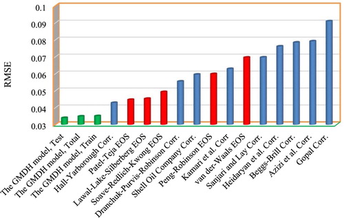
Figure 7. The predicting z-factor’s average absolute percent relative error correlations, GMDH models and EOSs.

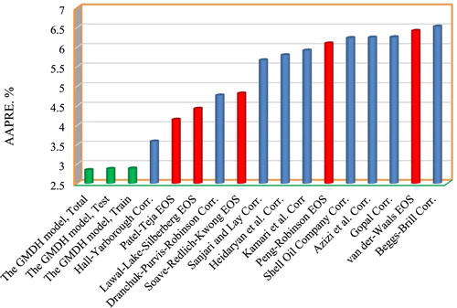
As can be seen in Figure 7, Beggs-Brill, Van der Waals, Gopal, Azizi, and Shell Oil Company models have the highest AAPRE values meaning that their predictions are less accurate than other models. It can be observed that the proposed model outperforms the former models by the AAPRE of 2.89%, 2.85%, and 2.88% for the training, testing and entire data sets, respectively. Further insight into performance of the model can be observed in Figure 6 with lower RMSE value compared to former published models.

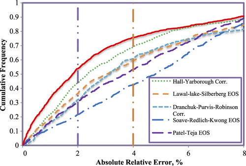
In order to investigate the accuracy of the GMDH model versus former models’ correlations, a cumulative frequency plot of the models are illustrated in Figure 8. This figure helps to achieve a better quantitative evaluation of the developed model when compared to the previously published models. This figure shows that the GMDH predicts nearly 52% of the data with an absolute relative error of 2%. More importantly, the model can predict 75% of the data points with an absolute relative error of only 4%. Thus, the model predict the gas compressibility factor with the smallest absolute relative error for any number of data points included in the predictions. This verifies the consistency of the developed GMDH model in accurately estimating gas compressibility factor within a wide range of reservoir conditions. The figure also shows that Hall-Yarborough correlation is the second model with high performance and accuracy that can estimate gas compressibility factor with small error values when any number of data points are considered. Another important finding from this figure is the comparison between the Lawal-lake-Silberberg EOS model and the Dranchuk-Purvis-Robinson correlation. While Lawal-lake-Silberberg EOS is more accurate in estimating gas compressibility factor for up to 50% of the data points, Dranchuk-Purvis-Robinson correlation becomes the superior model when more than 50% of the data points are included. This trend changes again when 80% or more of the data points are included.

Figure 8. Comparative analysis of the cumulative frequency versus absolute relative error.

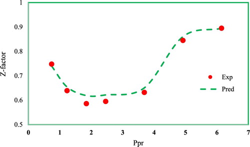
Finally, the predicted compressibility values by the GMDH model visually represented in Figure 9 against the experimental data at different pseudo-reduced pressure values and constant pseudo-reduced temperature of 0.7 to confirm the capability of the developed model in accurately estimating natural gas compressibility factor at different conditions. The experimental trend in this figure indicates that by increasing the pressure, gas compressibility factor first decreases and then increases. This trend has been accurately estimated by the developed GMDH model as shown by the dashed line in the same figure.

Figure 9. Variation of z-factor as a function of P_pr at T_pr = 1.19 for a gas sample.

6. Conclusions

In this work, GMDH was used to estimate the compressibility factor of natural gas. The GMDH model outperformed other models and provided higher accuracy at the various gas conditions. This was confirmed by measuring the RMSE, average absolute percent relative error, and regression coefficient to be 0.03, 2.88%, and 0.92, respectively. The Hall Yarborough correlation was determined as the second most accurate correlation for estimating the natural gas compressibility factor. Besides, the error distribution curve analysis indicated that the presented model in this study does not have an error trend when predicting very low and very high compressibility factor values. The experimental trend of gas compressibility factor showed that by increasing the pressure, the Z-factor first decreases and then increases. This trend was perfectly shown by the developed GMDH model in this work.

The results of this study show that generally, the correlations in the recent researches are based on limited data sets. Therefore, they are only able to predict the compressibility factor within limited ranges of pressure and temperature conditions. While the proposed GMDH model can accurately predict the natural different gas compressibility factor at low and high temperature and pressure conditions. The GMDH model is a data-driven based model, and its accuracy and reliability strongly depend on the data set used for its development. Using this model for temperature and pressure conditions beyond this study may lead to more error.

Disclosure statement

No potential conflict of interest was reported by the authors.

References

- Anitescu, C., Atroshchenko, E., Alajlan, N., & Rabczuk, T. (2019). Artificial neural network methods for the solution of second order boundary value problems. Computers, Materials & Continua, 59(1), 345–359.
- Azizi, N., Behbahani, R., & Isazadeh, M.A. (2010). An efficient correlation for calculating compressibility factor of natural gases. Journal of Natural Gas Chemistry, 19(6), 642–645.
- Beggs, D. H., & Brill, J. P. (1973). A study of two-phase flow in inclined pipes. Journal of Petroleum Technology, 25(05), 607–617.
- Brill, J., & Beggs, H. (1973). Two phase flow in pipes. Intercomp Course. The Hague: University of Tulsa.
- Chuntian, C., & Chau, K.-W. (2002). Three-person multi-objective conflict decision in reservoir flood control. European Journal of Operational Research, 142(3), 625–631.
- Dargahi-Zarandi, A., Hemmati-Sarapardeh, A., Hajirezaie, S., Dabir, B., & Atashrouz, S. (2017). Modeling gas/vapor viscosity of hydrocarbon fluids using a hybrid GMDH-type neural network system. Journal of Molecular Liquids, 236, 162–171.
- Dashtian, H., Bakhshian, S., Hajirezaie, S., Nicot, J.-P., & Hosseini, S. A. (2019). Convection-diffusion-reaction of CO2-enriched brine in porous media: A pore-scale study. Computers & Geosciences, 87(6), 234–245.
- Dranchuk, P. M., & Abou-Kassem, H. (1975). Calculation of Z factors for natural gases using equations of state. Journal of Canadian Petroleum Technology, 14(03), 97–124.
- Dranchuk, P. M., Purvis, R. A., & Robinson, D. B. (1973). Computer calculation of natural gas compressibility factors using the Standing and Katz correlation. Annual Technical Meeting.
- Dranchuk, P. M., Purvis, R. A., & Robinson, D. B. (1974). Computer calculation of natural gas compressibility factors using the Standing and Katz correlation. Annual Technical Meeting.
- Elsharkawy, A. M. (2004). Efficient methods for calculations of compressibility, density and viscosity of natural gases. Fluid Phase Equilibria, 218(1), 1–13.
- Elsharkawy, A. M., & Foda, S. G. (1998). EOS simulation and GRNN modeling of the constant volume depletion behavior of gas condensate reservoirs. Energy & Fuels, 12(2), 353–364.
- Firoozabadi, A. (1999). Thermodynamics of hydrocarbon reservoirs. New York: McGraw-Hill.
- Fotovatikhah, F., Herrera, M., Shamshirband, S., Chau, K.-W., Faizollahzadeh Ardabili, S., & Piran, M. J. (2018). Survey of computational intelligence as basis to big flood management: Challenges, research directions and future work. Engineering Applications of Computational Fluid Mechanics, 12(1), 411–437.
- Gopal, V. (1977a). Gas z-factor equations developed for computer. Oil and Gas Journal, 75(8), 8–13.
- Gopal, V. (1977b, August 8). Gas z-factor equations developed for computer. Oil and Gas Journal, 1977, 58–60.
- Guo, H., Zhuang, X., & Rabczuk, T. (2019). A deep collocation method for the bending analysis of Kirchhoff plate. CMC-Computers Materials & Continua, 58(2), 433–456.
- Hajirezaie, S., Hemmati-Sarapardeh, A., Mohammadi, A. H., Pournik, M., & Kamari, A. (2015). A smooth model for the estimation of gas/vapor viscosity of hydrocarbon fluids. Journal of Natural Gas Science and Engineering, 26, 1452–1459.
- Hajirezaie, S., Hemmati, S. A., & Ayatollahi, S. (2014). Soft computing model for prediction of sour and natural gas viscosity.
- Hajirezaie, S., Pajouhandeh, A., Hemmati-Sarapardeh, A., Pournik, M., & Dabir, B. (2017). Development of a robust model for prediction of under-saturated reservoir oil viscosity. Journal of Molecular Liquids, 229, 89–97.
- Hajirezaie, S., Wu, X., Soltanian, M. R., & Sakha, S. (2019). Numerical simulation of mineral precipitation in hydrocarbon reservoirs and wellbores. Fuel, 238, 462–472.
- Hall, K. R., & Yarborough, L. (1973). A new equation of state for Z-factor calculations. Oil and Gas Journal, 71(25), 82.
- Heidaryan, E., Moghadasi, J., & Rahimi, M. (2010). New correlations to predict natural gas viscosity and compressibility factor. Journal of Petroleum Science and Engineering, 73(1–2), 67–72.
- Hemmati-Sarapardeh, A., & Mohagheghian, E. (2017). Modeling interfacial tension and minimum miscibility pressure in paraffin-nitrogen systems: Application to gas injection processes. Fuel, 205, 80–89.
- Hemmati-Sarapardeh, A., Tashakkori, M., Hosseinzadeh, M., Mozafari, A., & Hajirezaie, S. (2016). On the evaluation of density of ionic liquid binary mixtures: Modeling and data assessment. Journal of Molecular Liquids, 222, 745–751.
- Kamari, A., Gharagheizi, F., Mohammadi, A. H., & Ramjugernath, D. (2016). A corresponding states-based method for the estimation of natural gas compressibility factors. Journal of Molecular Liquids, 216, 25–34.
- Kamari, A., Hemmati-Sarapardeh, A., Mirabbasi, S.-M., Nikookar, M., & Mohammadi, A. H. (2013). Prediction of sour gas compressibility factor using an intelligent approach. Fuel Processing Technology, 116, 209–216.
- Kamari, A., Pournik, M., Rostami, A., Amirlatifi, A., & Mohammadi, A. H. (2017). Characterizing the CO2-brine interfacial tension (IFT) using robust modeling approaches: A comparative study. Journal of Molecular Liquids, 246, 32–38.
- Kamari, A., Safiri, A., & Mohammadi, A. H. (2015). Compositional model for estimating asphaltene precipitation conditions in live reservoir oil systems. Journal of Dispersion Science and Technology, 36(3), 301–309.
- Kamyab, M., Sampaio, J. H., Jr., Qanbari, F., & Eustes, A. W., III (2010). Using artificial neural networks to estimate the z-factor for natural hydrocarbon gases. Journal of Petroleum Science and Engineering, 73(3–4), 248–257.
- Kumar, N. (2004). Compressibility factors for natural and sour reservoir gases by correlations and cubic equations of state. Texas: Texas Tech University.
- Lawal, A. (1999). Application of the Lawal-Lake-Silberberg equation-of-state to thermodynamic and transport properties of fluid and fluid mixtures.
- McCain, W. D., Jr. (2017). Properties of petroleum fluids. Florida: PennWell Corporation.
- McLeod, W. R. (1968). Applications of molecular refraction to the principle of corresponding states. Oklahoma: The University of Oklahoma.
- Moazenzadeh, R., Mohammadi, B., Shamshirband, S., & Chau, K.-w. (2018). Coupling a firefly algorithm with support vector regression to predict evaporation in northern Iran. Engineering Applications of Computational Fluid Mechanics, 12(1), 584–597.
- Patel, N. C., & Teja, A. S. (1982). A new cubic equation of state for fluids and fluid mixtures. Chemical Engineering Science, 37(3), 463–473.
- Peng, D.-Y., & Robinson, D. B. (1976). A new two-constant equation of state. Industrial & Engineering Chemistry Fundamentals, 15(1), 59–64.
- Robinson, R., Jr., & Jacoby, R. (1965). Better compressibility factors. Hydrocarbon Processing, 44(4), 141–145.
- Rostami, A., Kamari, A., Panacharoensawad, E., & Hashemi, A. (2018). New empirical correlations for determination of minimum miscibility pressure (MMP) during N2-contaminated lean gas flooding. Journal of the Taiwan Institute of Chemical Engineers, 91, 369–382.
- Sanjari, E., & Lay, E. N. (2012a). An accurate empirical correlation for predicting natural gas compressibility factors. Journal of Natural Gas Chemistry, 21(2), 184–188.
- Sanjari, E., & Lay, E. N. (2012b). Estimation of natural gas compressibility factors using artificial neural network approach. Journal of Natural Gas Science and Engineering, 9, 220–226.
- Shariaty, S., Khorsand Movaghar, M. R., & Vatandoost, A. (2019). A new model for estimating the gas compressibility factor using group method of data handling algorithm (case study). Asia-Pacific Journal of Chemical Engineering, 14(3), e2307.
- Shateri, M., Ghorbani, S., Hemmati-Sarapardeh, A., & Mohammadi, A. H. (2015). Application of Wilcoxon generalized radial basis function network for prediction of natural gas compressibility factor. Journal of the Taiwan Institute of Chemical Engineers, 50, 131–141.
- Simon, R., & Briggs, J. E. (1964). Application of Benedict-Webb-Rubin equation of state to hydrogen sulfide-hydrocarbon mixtures. AIChE Journal, 10(4), 548–550.
- Soave, G. (1972). Equilibrium constants from a modified Redlich-Kwong equation of state. Chemical Engineering Science, 27(6), 1197–1203.
- Standing, M. B., & Katz, D. L. (1942). Density of natural gases. Transactions of the AIME, 146(01), 140–149.
- Taherei Ghazvinei, P., Hassanpour Darvishi, H., Mosavi, A., Yusof, K. b. W., Alizamir, M., Shamshirband, S., & Chau, K.-w. (2018). Sugarcane growth prediction based on meteorological parameters using extreme learning machine and artificial neural network. Engineering Applications of Computational Fluid Mechanics, 12(1), 738–749.
- Van Der Waals, J. D., & Rowlinson, J. S. (2004). On the continuity of the gaseous and liquid states. Newyork: Courier Corporation.
- Van der Waals, J. D., Threfall, R., Adair, J. F., & Roth, F. (1873). The continuity of the liquid and gaseous states.
- Whitson, C. H., & Torp, S. B. (1981). Evaluating constant volume depletion data. SPE Annual Technical Conference and Exhibition.
- Wichert, E., & Aziz, K. (1972). Calculate Zs for sour gases. Hydrocarbon Processing, 51(5), 119–122.
- Yaseen, Z. M., Sulaiman, S. O., Deo, R. C., & Chau, K.-W. (2019). An enhanced extreme learning machine model for river flow forecasting: State-of-the-art, practical applications in water resource engineering area and future research direction. Journal of Hydrology, 77, 324–340.