Numerical investigation of a double-circulation system for cuttings transport in CBM well drilling using a CFD-DEM coupled model

ABSTRACT

In this study, a numerical model of a partial wellbore is developed by coupling computational fluid dynamics (CFD) with the discrete element method (DEM) in order to simulate the operation of a double-circulation system (DCS) in coalbed methane (CBM) well drilling, which is a novel technique used for cuttings transport. The values of the flow field are computed by a fluid solver and the motions of the particle phase are calculated by the DEM, for which an additional multi-sphere particle model is integrated. After verification of the model, the analysis centers on the working mechanism, the DCS parameters, and optimization of the angle θ of the injection nozzles, which is the most critical parameter affecting the efficiency of the DCS. Simulations reveal the working details of the DCS and prove its applicability to cuttings transport, especially in the curved and horizontal parts of the well. The effects of viscosity and particle size are investigated, and a low-viscosity drilling fluid is recommended. The optimal range for θ is obtained as 30° to 50°. This work provides a reference for the engineering application of DCSs, and by feedback from drilling sites the reliability of the results can be verified.

KEYWORDS:

• CBM drilling
• double-circulation
• CFD-DEM
• multi-sphere algorithm
• non-spherical particles

1. Introduction

The use of gas in underbalanced drilling (UBD) has become common over the last decade, the engineering purpose of which is to promote the return of drilling fluid from the well bottom while keeping the wellbore pressure lower than the formation pressure (Mykytiw, Davidson, Shell UBD Global Implementation Team [SUGIT], Frink, & Blade Energy Partners [BEP], 2003; Paredes et al., 2010; Suryanarayana, Hasan, & Hughes, 2004). UBD with gas injection has received much focus and been widely applied around the world due to its many merits, one of which is that the injection of gas can offer assistance with cuttings transport. However, due to the high compressibility of gas compared with liquid, gas injection is more volatile – especially when local collapses occur in the well wall or when the content of the cuttings in the drilling fluid fluctuates, both of which are almost inevitable in coalbed methane (CBM) drilling due to the fragility of coal rock. Worse still, uncontrolled gas pressure may induce pressure jumps at the bottom of the well, which can potentially aggravate the collapse of the well wall (Akbarian et al., 2018; Ghalandari, Koohshahi, Mohamadian, Shamshirband, & Chau, 2019; Guo, Yao, & Ai, 2008; Nguyen, Somerville, & Smart, 2009; Zhu, Liu, & Tong, 2011).

Given the above, adjustments continue to be made to the equipment and tools used in UBD. One of these changes is the use of a double-circulation system (DCS) for CBM well drilling, in which the gas is replaced with viscous liquid. DCSs have been applied to CBM well drilling in the Qinshui basin in China, and encouraging results have been obtained (Yang et al., 2015, 2017). However, currently there are few studies on the working mechanism of DCSs in relation to cuttings transport, so the relevant numerical simulations are carried out in the present work, which is expected to provide some guidance on and perhaps improvements to the further application of DCSs.

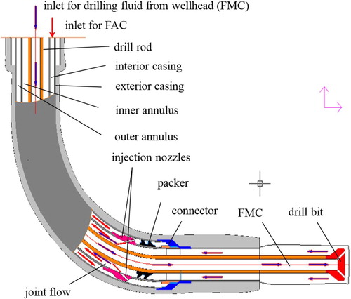
The novel DCS is developed mainly to provide assistance with removing the cuttings accumulations resulting from a fast drilling rate that tend to build up in the horizontal and curved sections of the wellbore, which can cause complications like sticking that can result in drilling accidents. The working mechanism of a DCS is illustrated by Figure 1. After the second well completion, the interior casing and accompanying tools such as the centralizer, packer, and injection joint are lowered to the connector, which is used to connect the interior casing to the exterior casing. During the drilling process, the flow of main circulation (FMC) is injected from the wellhead and travels down the interior of the drill rod, coming out from the drill bit into the inner annulus space. Simultaneously, the flow of assisted circulation (FAC) is injected from the wellhead into the outer annulus and flows through the nozzles, meeting the FMC in the inner annulus where the joint flow returns to the wellhead carrying the cuttings.

Figure 1. Working mechanism of a double-circulation system (DCS) for drilling.

Cuttings transport has been studied by many researchers. Ford, Peden, Oyeneyin, Gao, and Zarrough (1990) and Tomren, Iyoho, and Azar (1986) conducted experimental studies of cuttings transport in directional (or inclined) wells. Akhshik, Behzad, and Rajabi (2015) coupled computational fluid dynamics (CFD) with the discrete element method (DEM) to simulate cuttings transport in well drilling and examine the influence of critical parameters such as the drill pipe rotation. Capo, Yu, Miska, Takach, and Ahmed (2006) and Chen et al. (2007) carried out experimental studies on cuttings transport with foam, in which tests were conducted to determine the effects of parameters such as the inclination angle, foam quality, and velocity. Duan, Miska, Yu, Takach, and Ahmed (2007) investigated the effects of factors such as the critical re-suspension velocity (CRV), critical fluid velocity (CFV), and critical deposition velocity (CDV) on sand-sized solids moving in inclined wells. Ozbayoglu, Saasen, Sorgun, and Svanes (2010) used experiments and empirical formulae to obtain the CFV needed to stop the development of a stationary bed in highly inclined wellbores. Many other researchers have also undertaken experimental and theoretical studies on the dynamics of cuttings or particles moving in fluids (Kelessidis & Bandelis, 2004; Li et al., 2013; Manzar & Shah, 2009; Ozbayoglu, Erge, & Ozbayoglu, 2018; Sanchez, Azar, & Bassal, 1999; Shao, Liu, Lin, Xu, & Yan, 2017; Song, Guan, & Chen, 2009).

Due to the material variations in coal, during the drilling of coal stratum, large, non-spherical cuttings often emerge. Given this complexity, CFD-DEM coupled models are often adopted to accomplish the simulation of such fluid–particle interactions. Zhao and Shan (2013) simulate the fluid–particle interactions in mining and geotechnical engineering using a CFD-DEM model. Complex geometries are studied by Liu, Bu, and Chen (2013), who coupled the DEM with the ANSYS Fluent software to develop a CFD-DEM model. Akhshik and Rajabi (2018) focus on the shapes of the particles, building disc-shaped, cubic-shaped, and round-shaped particles in order to study the differences in their movement processes. In the work of Zhong, Yu, Liu, Tong, and Zhang (2016), recent efforts in developing the DEM to study the interactions of non-spherical particles and fluids are used to examine contact detection, coupling methodologies, collision dynamics, and fluid–particle forces.

Many other researchers have also made important contributions to the application of CFD-DEM models (Carlos Varas, Peters, & Kuipers, 2017; Di Renzo & Di Maio, 2004; He, Bayly, & Hassanpour, 2018; Issakhov, Bulgakov, & Zhandaulet, 2019; Zeng, Li, & Zhang, 2016). However, limited research has been carried out on the interactions of fluid and non-spherical particles, with few studies focusing on the application of DCSs to CBM drilling. Therefore, this study seeks to help to fill this important gap in the literature.

2. Model description

In this section, models for the fluid phase and the particle phase – as well as how they interact – are introduced. Based on the outstanding theoretical works of Kloss, Goniva, Hager, Amberger, and Pirker (2012), the components of the flow field are calculated using OpenFOAM (OpenCFD Ltd., 2009), and LIGGGHTS (2011) is adopted as the DEM solver.

2.1. Flow field

In this coupled CFD-DEM model, the Eulerian approach in OpenFOAM is adopted for computing the incompressible flow field. The dispersed phase in the fluid is considered by the volume fraction (VF) ϵ_f in the mass conservation equation and the momentum conservation equation, which are respectively given as: (1) $\frac{\mathrm{\partial }\left({\epsilon }_f{\rho }_f\right)}{\mathrm{\partial }t}+\mathrm{\nabla }\cdot \left({\epsilon }_f{\rho }_f{\mathit{u}}_f\right)=0,$(1) (2) $\begin{array}{rl}& \frac{\mathrm{\partial }\left({\epsilon }_f{\rho }_f{\mathit{u}}_f\right)}{\mathrm{\partial }t}+\mathrm{\nabla }\cdot \left({\epsilon }_f{\rho }_f{\mathit{u}}_f{\mathit{u}}_f\right)=-{\mathrm{\nabla }}_p+\mathrm{\nabla }\cdot \left({\mu }_f{\epsilon }_f\mathrm{\nabla }{\mathit{u}}_f\right)\\ & -{\epsilon }_f{\rho }_f\mathit{g}-\mathit{S}\mathbf{,}\end{array}$(2) where ρ_f is the fluid density, t is the time, u_f is the fluid velocity, p is the fluid pressure, μ_f is the fluid viscosity, ϵ_f is the fluid volume fraction, g is the gravity, and S is the interaction forces.

In one interaction fluid cell, the interaction forces S are the joint forces of the fluid exerted on the particles: (3) $S=\frac{1}{\mathrm{\Delta }V}\sum _{i=1}^n{\mathit{F}}_{f,i},$(3) where ΔV is the cell volume, F_f,i is the fluid forces, and n is the number of particles.

2.2. Particle motion

The motion of particle i is composed of translation and rotation, the governing equation for which is Newton’s Law: (4) $\left.\begin{array}{l}{m}_i\frac{dU\left(t\right)}{dt}={\mathit{F}}_i\\ I_i\frac{d\mathrm{\Omega }\left(t\right)}{dt}={\mathit{T}}_i\end{array}\right\}\mathrm{\forall }t>0,$(4) where $m_i$ is the particle mass, $I_i$ is the inertia moment, $F_i$ is the total force, $T_i$ is the total torque, $\mathrm{\Omega }\left(t\right)$ is the angular velocity, and F_i is the joint force consisting of the pressure gradient force, buoyancy force, contact force with other particles, fluid drag force, and lift force. Finally, the particle velocity can be obtained by $U\left(t\right)=dX\left(t\right)/dt$.

The fluid drag force exerted on a non-spherical particle can be calculated as follows (Shook & Roco, 1991): (5) $\begin{array}{rl}{\mathbf{F}}_D& =A_p({\mathbf{u}}_f-{\mathbf{u}}_p),\\ A_p& =0.75C_D\frac{(1-\alpha ){\rho }_f|{\mathbf{u}}_f-{\mathbf{u}}_p|}{d_p}{\alpha }^{-1.65}\end{array}$(5) where d_p is the particle diameter and C_D is the drag coefficient, which is calculated by its sphericity ζ (ζ = 0.786 for flaky particles) and is given as follows (Alexandrou, Menn, Georgiou, & Entov, 2003; Chien, 1994): (6) $\begin{array}{r}\begin{array}{rl}{C}_D& =\frac{30.0}{{\text{Re}}_{HB}}+\frac{67.289}{e^{5.03\zeta }}\\ {\text{Re}}_{HB}& =\frac{{\rho }_f{|{\mathbf{u}}_f-{\mathbf{u}}_p|}^{2-n}{d_p}^n/k}{1+0.916\left({\tau }_0/k\right)\left(d_p/|{\mathbf{u}}_f-{\mathbf{u}}_p|\right)}\\ \zeta & =\frac{A_s}{A_n}\end{array}\end{array}$(6)

where n is the power-law component, τ₀ is the yield stress, k is the consistency factor, A_s is the surface area of the equivalent spherical particle with the same volume as the non-spherical particle, and A_n is the surface area.

The drag torque is given as follows (Sommerfeld, 2000): (7) $\begin{array}{r}\begin{array}{rl}{T}_D^p& =\frac{{\rho }_p}{2}{\left(\frac{d_p}{2}\right)}^5{C}_{DR}|{\omega }_r|{\omega }_{{}_r}\mathbf{,}\\ C_{DR}& =\left\{\begin{array}{l}\frac{12.9}{{{\text{Re}}_r}^{0.5}}+\frac{128.4}{{\text{Re}}_r},34\le {\text{Re}}_r\le 1000\\ \frac{64\pi }{{\text{Re}}_r},{\text{Re}}_r<32\end{array}\right.,\\ {\text{Re}}_r& =\rho {d_p}^2|{\omega }_r|/\mu \end{array}\end{array}$(7) where C_DR is the rotational drag coefficient, ω_r is the relative angular velocity, and Re_r is the Reynolds number of rotation.

T_ij is the total torque in the particle interaction, which can be obtained as follows: (8) ${\mathit{T}}_{ij}={\mathit{R}}_{ij}\times {\mathit{f}}_{ij,c}$(8) where R_i is the vector from the mass center of the ith particle to the contact point and f_ij,c is the contact force between two particles. If there are k_i particles in contact with the ith particle at the same time then the total torque on the ith particle is T_ij.

The buoyancy force is given as follows: (9) ${\mathit{F}}^b=\frac{{\rho }_f}{{\rho }_p}{m}_s\mathbf{g}$(9) where m_s is the total mass given by Equation (12) below.

The lift force from the fluid exerted on the multi-sphere particle is given as follows (Mei, 1992; Saffman, 1965; Sommerfeld, 2000), which is from that of the equivalent spherical particle: (10) $\begin{array}{r}\begin{array}{rl}{\mathbf{F}}_S& =0.125C_L\pi {\rho }_f{d_p}^3\left[({\mathbf{u}}_f-{\mathbf{u}}_p)\times {\omega }_f\right],\\ C_L& =\left\{\begin{array}{l}\frac{4.113}{{{\text{Re}}_s}^{0.5}}\left[(1-0.331{\vartheta }^{0.5})e^{-{\mathrm{R}\mathrm{e}}_{HB}/10}+0.331{\vartheta }^{0.5}\right],\\ {\text{Re}}_{HB}\le 40\\ \frac{0.216}{{{\text{Re}}_s}^{0.5}}\left(\vartheta \cdot {\text{Re}}_{HB}\right),{\text{Re}}_{HB}>40\end{array}\right.,\\ {\text{Re}}_s& ={\rho }_f{d_p}^2|{\omega }_f|/\mu \end{array}\end{array}$(10) where ${\omega }_f$ is given by ${\omega }_f=\mathrm{\nabla }\times {\mathbf{u}}_f$ and $\vartheta =0.5{\text{Re}}_s/{\text{Re}}_{HB}$ (0.005 < $\vartheta$ < 0.4).

The rotational lift force is calculated as follows: (11) $\begin{array}{l}{\mathbf{F}}_M=0.125C_{LM}\pi {\rho }_f{d_p}^3|{\mathbf{u}}_f-{\mathbf{u}}_p|\left({\mathbf{u}}_f-{\mathbf{u}}_p\right)|{\omega }_r|\mathbf{/}{\omega }_{{}_r},\\ C_{LM}=0.45+\left(\frac{{\text{Re}}_r}{{\text{Re}}_{HB}}-0.45\right)e^{-0.568{{\mathrm{Re}}_r}^{0.4}{{\mathrm{Re}}_{HB}}^{0.3}}\end{array}$(11) where C_LM is the coefficient for the rotational lift force.

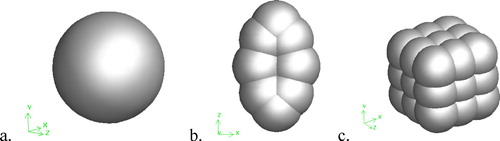
The statistical analysis conducted on the cuttings samples from the CBM drilling site revealed that most of the cuttings are flaky rather than spherical. Therefore, non-spherical particles need to be modeled for considering the effects of the particle shape on cuttings transport. In this study, the non-spherical particles are built from multiple spheres that are rigidly connected (Kruggel-Emden, Rickelt, Wirtz, & Scherer, 2008). Figure 2 shows the three particle shapes used in the present study. In the multi-sphere approach, the non-spherical particle i is composed of multiple spheres which overlap one another. The mass $m_s$, gravity center $O_i$, and inertia moment $I_i$ can be obtained as follows: (12) $m_s=\sum _{a=1}^N{m}_{s,a},$(12) (13) $O_i=\sum _{a=1}^N\left(O_{i,a}{m}_{s,a}\right)/m_s$(13) (14) $\begin{array}{r}{I}_i=\left[\begin{array}{cc}& \sum I_{i,a}+\sum m_{s,a}(O_{i,a,Y}^2+O_{i,a,Z}^2)\\ & -\sum m_{s,a}{O}_{i,a,X}{O}_{i,a,Y}\\ & -\sum m_{s,a}{O}_{i,a,X}{O}_{i,a,Z}\end{array}\right.\\ \begin{array}{cc}& -\sum m_{s,a}{O}_{i,a,X}{O}_{i,a,Y}\\ & \sum I_{i,a}+\sum m_{s,a}(O_{i,a,X}^2+O_{i,a,Z}^2)\\ & -\sum m_{s,a}{O}_{i,a,Y}{O}_{i,a,Z}\end{array}\\ \left.\begin{array}{cc}& -\sum m_{s,a}{O}_{i,a,X}{O}_{i,a,Z}\\ & -\sum m_{s,a}{O}_{i,a,Y}{O}_{i,a,Z}\\ & \sum I_{i,a}+\sum m_{s,a}(O_{i,a,X}^2+O_{i,a,Y}^2)\end{array}\right]\end{array}$(14) where $N$ is the number of spheres in the non-spherical particle i, the subscript a is the kth spherical body, and $O_{i,a,X}$, $O_{i,a,Y}$, and $O_{i,a,Z}$ are the distances from the principle axes of the particle to the center of sphere a.

Figure 2. Particle models used in the multi-sphere approach: (a) spherical; (b) flaky; (c) cubic.

2.3. Particle contact algorithm

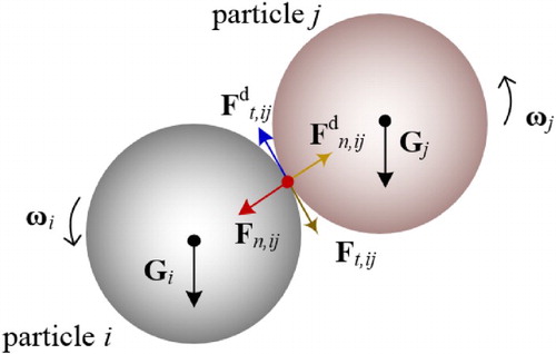
Figure 3 shows the contact mechanism between the ith particle and the jth particle. The joint contact force ${\mathbf{F}}_{c,i}^p$ is adopted from the work of Di Renzo and Di Maio (2004): (15) ${\mathbf{F}}_{c,i}^p={\mathbf{F}}_{n,ij}+{\mathbf{F}}_{n,ij}^d+{\mathbf{F}}_{t,ij}+{\mathbf{F}}_{t,ij}^d$(15)

where F_n,ij is the normal component and is expressed as: (16) ${\mathbf{F}}_{n,ij}=\frac{4}{3}{E}^{\ast }\sqrt{R^{\ast }}{\delta }_{n,ij}^{3/2}$(16) where $E^{\ast }$ is the equivalent Young’s modulus ($E^{\ast }=\left[\right(1-{\upsilon }_i^2)/E_i+(1-{\upsilon }_j^2)/E_j{]}^{-1}$), R* is the equivalent radius ($R^{\ast }=(2/d_p+2/d_q{)}^{-1}$), ${\delta }_{n,ij}$ is the normal overlap, E is the Young’s modulus, υ is the Poisson ratio, and d is the particle radius.

Figure 3. Forces between two contacting particles i and j.

The normal damping force F_n,ij is given as follows: (17) ${\mathbf{F}}_{n,ij}^d=-2\sqrt{\frac{5}{6}}\frac{\ln e}{\sqrt{{(\ln e)}^2+{\pi }^2}}\sqrt{S_{n,ij}{m}^{\ast }}{\mathbf{v}}_{n,pq}$(17) where the normal stiffness $S_{n,ij}$ is given by $S_{n,ij}=2E^{\ast }\sqrt{R^{\ast }{\delta }_{n,ij}}$, $m^{\ast }$ is the equivalent mass calculated from the masses of two contacting particles m_i and m_j ($m^{\ast }=[1/m_i+1/m_j{]}^{-1}$), v_n,pq is the normal component of the relative velocity of the contact point, and e is the coefficient of restitution.

The tangential component of the contact force F_t,ij and the tangential damping forces ${\mathbf{F}}_{t,ij}^d$ are respectively expressed as follows: (18) ${\mathbf{F}}_{t,ij}=\left\{\begin{array}{l}-{\delta }_{t,ij}{S}_{t,ij},|{\mathbf{F}}_{t,ij}|<{\mu }_s{\mathbf{F}}_{n,ij}\\ {\mu }_s|{\mathbf{F}}_{n,ij}|\frac{{\text{v}}_{t,pq}}{|{\text{v}}_{t,pq}|},|{\mathbf{F}}_{t,ij}|\ge {\mu }_s{\mathbf{F}}_{n,ij}\end{array}\right.$(18) (19) ${\mathbf{F}}_{t,ij}^d=-2\sqrt{\frac{5}{6}}\frac{\ln e}{\sqrt{{(\ln e)}^2+{\pi }^2}}\sqrt{S_{t,ij}{m}^{\ast }}{\text{v}}_{t,pd}$(19) where S_t,ij is the tangential stiffness, μ_s is the sliding friction coefficient, and v_t,pq is the relative tangential velocity at the contact point.

2.4. CFD-DEM coupled algorithm

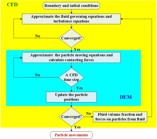
In the present CFD-DEM coupled approach, a CFD solver in OpenFOAM and a DEM solver in LIGGGHTS were adopted to calculate the values of the flow field and the particle motions, respectively. The procedure for the coupled approach is shown in Figure 4. First, the fluid’s continuity, momentum, and turbulence (using the k-ϵ turbulence scheme) are approximated by the CFD solver until they have converged. In the cell containing the particles, the fluid forces acting on each particle are further calculated on the basis of the VF of the particles. The particle positions and velocities are approximated by the DEM solver after the convergence of the CFD solver. When the current time step in the CFD solver is over, the particles’ updated values are returned to the grid cells, then the VF of the fluid and the fluid forces are calculated. The CFD solver then iterates over a new time step and the process repeats until the solution converges.

Figure 4. Procedures of the CFD-DEM coupled approach.

3. Verification cases

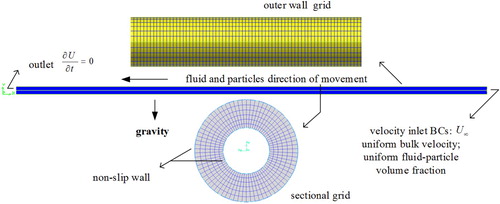
Experimental data from the work of Shao et al. (2017) were used to verify the developed CFD-DEM model, from which the CFV V_c was used. Due to the long, flaky cuttings obtained in the samples from a coal seam in a typical CBM well (ZS-1H) using a common polycrystalline diamond compact (PDC) bit (Figure 5), both flaky and spherical particles were adopted in the verification cases. The flaky particles are composed of eight identical smaller spheres with their centers placed on one shared plane. The volume of the flaky particle is the same as that of the spherical particle so that the two can be compared; for example, for a 4-mm spherical particle the diameter of the small spheres in the equivalent flaky particle is 2.464 mm and the sphericity ζ is 0.786. The simulation model is geometrically identical to a CBM wellbore with an external diameter of 140 mm and an internal diameter of 63 mm. The length of the horizontal part of the numerical wellbore is 25 m. The density, Poisson’s ratio, and shear modulus of the cuttings are 2300 kg/m³, 0.25, and 1.96 GPa, respectively. The chosen particle sizes are 2, 4, and 6 mm. The density and viscosity of the fluid are 1.0 g/cm³ and 0.01 cm²/s, respectively. The mesh and boundary conditions can be found in Figure 6. The CFV V_c was adopted for making a comparison regarding which is the right value for the flow velocity when all of the cuttings are carried out of the annulus in an accelerating flow.

Figure 5. Cuttings images: (a) cuttings sample; (b) spherical particle model; (c) flaky particle model.

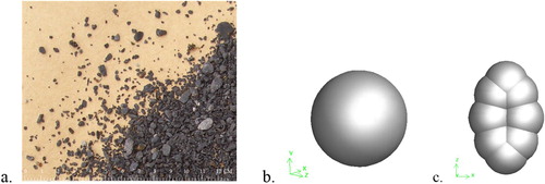
Figure 6. Simulation model and grids.

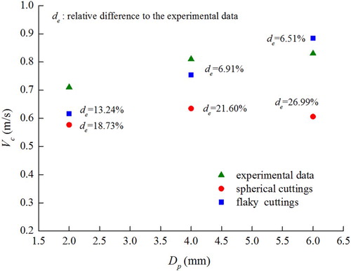
The CFVs from the CFD-DEM model simulations and the experiments of Shao et al. (2017) are compared in Figure 7. It can be seen that the V_c values for both the spherical and the flaky particles rise as the size of the cuttings increases, which is in agreement with the experimental data. However, there are considerable differences between the spherical and flaky particles; the V_c values of the flaky particles are closer to the experimental values, with an average deviation of 8.89%, whereas the average deviation of the spherical particles is 22.44%. The comparison therefore shows that flaky particles are much better suited for use in the simulations. Moreover, the acceptable deviation for flaky particles indicates that the CFD-DEM coupled approach is adequate for simulating cuttings transport.

Figure 7. Comparison of the present simulated CFVs and the experimental CFVs of Shao et al. (2017).

4. Numerical work on cuttings transport

4.1. CFD-DEM model

In this section, a simulated model of a partial wellbore is built based on real-world drilling data from CBM Well ZS-3H in the Qinshui basin, incorporating the well trajectory data, wellbore sizes, and drilling parameters. The model was expected to reveal how to improve the assisted circulation of cuttings transport in the wellbore, as well as how to optimize the injection nozzle used in the assisted circulation.

The CFD-DEM model is shown in Figure 8, and the parameters used are listed in Table 1. Four injection nozzles are placed evenly on one cross-section of the wellbore, and the angle between the axis of the wellbore and the nozzle is indicated by θ. The initial VF of the cuttings in the inlet is estimated by the normal drilling rate (5.0 m/h) of Well ZS-3H, and the cuttings particles are injected sequentially from the bottom inlet. Among the total 5,861,045 cells, the length of the smallest cell is 0.02 m. The time steps for the CFD and DEM solver are 0.001 and 0.0001, respectively.

Figure 8. Whole-well model for the double-circulation system (DCS): (a) overall well model; (b) boundary conditions; (c) flaky particle model used.

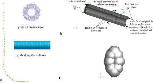
Table 1. Parameters used for the CFD-DEM simulation model.

Parameter (unit)	Value	Parameter (unit)	Value
Well depth (m)	1000.00	Depth of injection nozzles (m)	780.00
FMC (l/s)	15.00	Diameter of injection nozzles (mm)	10.00
FAC (l/s)	14.00	Injection angle θ (°)	30.00
Diameter of exterior casing (mm)	177.80	Input VF of cuttings (%)	0.20
Diameter of interior casing (mm)	130.00	Cuttings diameter (mm)	2.00
Diameter of drill rod (mm)	88.90	Density of cuttings (g/cm^3)	2.30
Rotation speed of drill rod (rad/s)	7.33	Poisson’s ratio	0.23
Density of drilling fluid (g/cm^3)	1.06	Shear modulus (GPa)	1.96
Maxwell funnel viscosity (s)	45.00	Rolling friction coefficient	0.01

4.2. Simulation of cuttings transport under double circulation

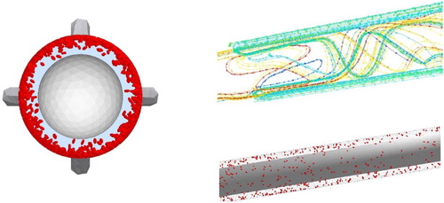
Figure 9 shows the local concentration of cuttings around the injection nozzles. From the contour of the partial well structure, there is a local cuttings heap underneath the nozzle, which is verified by the VF of the cuttings in the cross-sections. The maximum VF of the cuttings underneath the nozzle draws near to 0.3%, while above the nozzle it stays at less than 0.2% – that is to say, with the help of assisted circulation, the local cuttings accumulations around the nozzle can be cleared away. In Figure 10, flow lines show how the flow from the main inlet meets with the injection stream from the nozzles; the joint stream then moves forward in the annulus space between the interior casing and the drill rod while rotating around the rod. Moreover, another phenomenon occurs: due to the difference between the narrow space in the nozzle and the relatively larger well annulus space, the pressure changes and gives rise to a local vortex (see Section 5 below for more details).

Figure 9. Local concentration of cuttings around the injection nozzles.

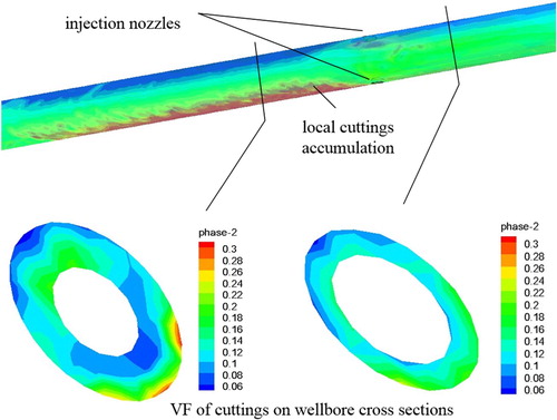
Figure 10. Drilling fluid path lines around the nozzles and flaky particles in the wellbore annulus.

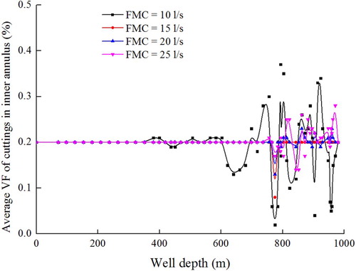
By extracting the average value of the cuttings’ upward speed in the wellbore inner annulus, the curve of the speed versus the well depth under different values of FAC is obtained. Figure 11 demonstrates that the FAC and other parameters are consistent with those in Table 1. As the assisted circulation flow increases, the speed of the cuttings is obviously promoted above the nozzles, which is indicated by the lifted sections of the curves (for a well depth of less than 780 m). Figure 12 shows the effects of the FMC on the velocity of the cuttings. It can be seen that in the sections of the wellbore underneath the nozzles where only the main circulation is present, the cuttings’ speed is boosted with an increase in FMC, although this increase is not steady.

Curves of the average VF of the cuttings in the wellbore inner annulus versus the well depth are given in Figure 13. Consistent to what is shown in Figure 12, the diminution of the VF of the cuttings around the nozzles with an increase in the FMC indicates the positive effect of the main circulation on cuttings transport. However, the VF distribution is dispersed in the curved and horizontal sections of the well (for a well depth of greater than 600 m) but evenly spread in the vertical section, which suggests that a local concentration of cuttings is more likely to occur in the curved and horizontal sections of the well without the help of assisted circulation.

Figure 11. Upward velocity of cuttings vs well depth with varying FAC values.

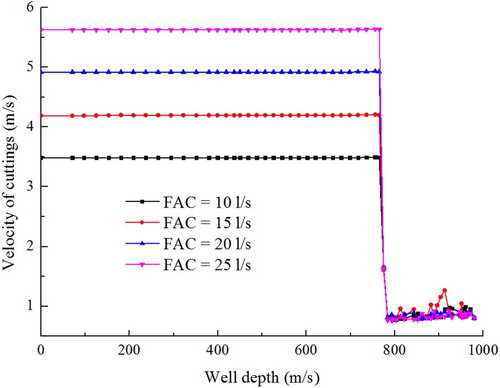
Figure 12. Upward velocity of cuttings vs well depth with varying FMC values.

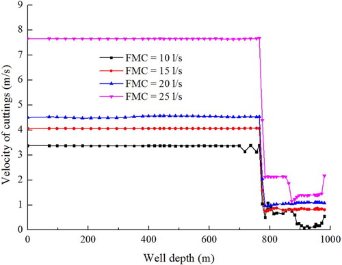
Figure 13. Average VF of the cuttings vs well depth with varying FMC values.

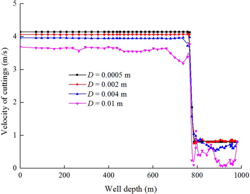
The influence of the cuttings size can be seen in Figure 14, which shows how the average VF of the cuttings at different well depths varies with different cuttings diameters (D). With the chosen FAC, FMC, fluid viscosity, and other parameters, for smaller cuttings (D < 0.01 m) only the VF of the cuttings underneath the nozzles is distributed unevenly, whereas for larger cuttings (D = 0.01 m) the VF of the cuttings is dispersed around the entire wellbore, which means that the wellbore is much more prone to build-ups of local heaps of larger cuttings. Figure 15 shows a decrease in the velocity of the cuttings with an increase in their size, indicating that the drilling fluid has a poor carrying ability for larger cuttings.

Figure 14. Average VF of the cuttings vs well depth with varying cuttings sizes.

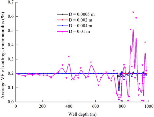
Figure 15. Upward velocity of cuttings vs well depth with varying cuttings sizes.

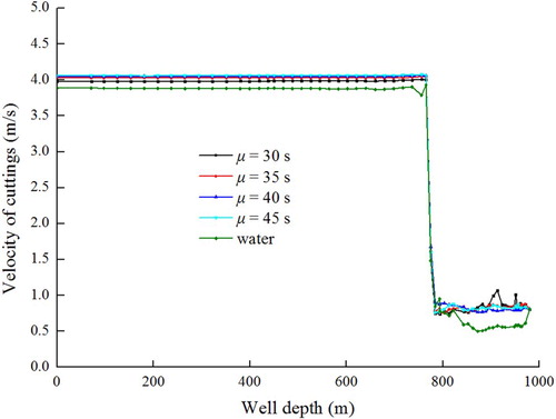
The effect of the drilling fluid viscosity (μ) is also considered. Curves of the average VF of the cuttings versus the well depth under varying drilling fluid viscosities are given in Figure 16, which shows that the curves are relatively smooth and steady for well depths of less than 780 m but fluctuate for depths of greater than 780 m. The contrast still manifests the improvement in cuttings transport performance resulting from assisted circulation. However, in the fluctuating sections, the fluid exhibits a better cuttings carrying ability when it is more viscous, because the points for water are obviously more dispersed.

Figure 16. Average VF of the cuttings with varying drilling fluid viscosities.

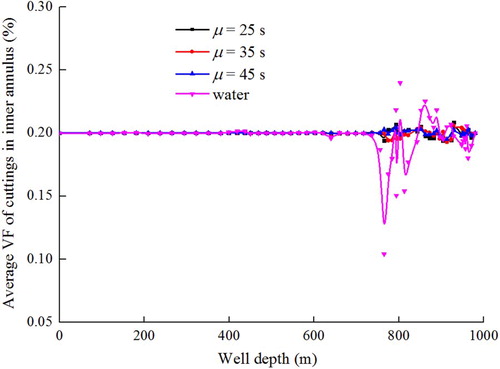
The positive impact on cuttings transport from increasing the fluid viscosity can also be seen in Figure 17. With the other parameters fixed and only the viscosity rising, the cuttings move slightly faster – but there is not much difference between the low and high viscosity fluids in performance. Thus, for cuttings transport in drilling when using a DCS, drilling fluid with a relatively low viscosity is sufficient and recommended.

Figure 17. Upward velocity of cuttings with varying drilling fluid viscosities.

5. Optimization of the angle θ of the injection nozzle

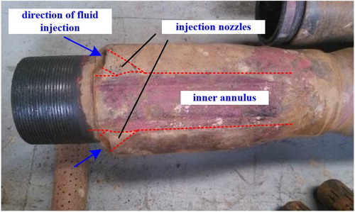
The joint between the exterior and interior casing of the wellbore, where the injection nozzles are located as well as where the FAC meets the FMC, is the key part of the system. Figure 18 shows an example of a casing joint that has been in service. To date, little research has been conducted on this joint, and the parameters of the nozzles have been especially neglected, among which the angle θ is most worthy of study. In this section, some computations are carried out and suggestions for optimization are given.

Figure 18. Casing joint with injection nozzles.

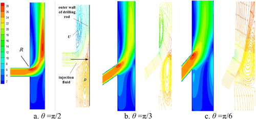
Based on the structural symmetry of the joint, a lengthways 2D model with a nozzle and annulus space was built. The diameter of the nozzles is 0.02 m and the injection angle θ varies in the range of 0 to π/2. The length of the model is 2.2 m, the annulus distance is 0.0445 m, and the other dimensions can be found in Table 1. The assistant boundary conditions shown in Figure 8(b) are adopted. As can be seen in Figure 19, fluid from the assisted circulation is injected into the inner annulus at different injection angles θ, and when it meets the fluid from the main circulation, the maximum flow velocity always occurs at the upper point of the joint (point R in Figure 19). Local vortexes form at the point where the FAC meets the FMC. When the injection angle θ is π/2 or π/3, vortexes occur both above and below the nozzle, respectively denoted by regions U and D in Figure 19(a) and (b). The vortexes are produced by the FAC impacting on the outer surface of the drill rod. However, when the injection angle is small enough (θ = π/6), the upper vortex in region U disappears and only the lower vortex in region D remains (Figure 19(c)).

Figure 19. Drilling fluid velocity contours and streamlines around the nozzle for: (a) θ = π/2; (b) θ = π/3; (c) θ = π/6.

When the injection flow from the nozzle is moving at a high speed, it impacts on the outer surface of the drill rod. In Figure 20 it can be seen that with an injection angle of θ = π/2, the direction of injection is perpendicular to the axis of the drill rod, and thus has the smallest impact distance. At this angle, the injection flow generates the greatest momentum in the drill rod and may cause fairly strong erosion on the surface, while the strongest vortex forms underneath the nozzle and opposes the cuttings’ upward movement.

Figure 20. Shear stress on the outer surface of the drill rod under different injection angles θ.

Note: Y represents the distance to the cross point of the wall of the drill rod and the axis of the nozzle with θ = π/2, which is denoted in Figure 19(a) by the arrow labelled ‘injection fluid’.

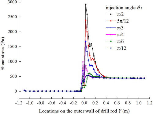
Figure 21 shows the contours of the VF of the cuttings in the inner annulus around the nozzle for several different injection angles. It can easily be seen that the maximum value of the VF occurs at the edge of the vortex underneath the nozzle. Additionally, the concentration region (the red region in Figure 21) is located right next to the drill rod.

Figure 21. VF of the cuttings under different injection angles: (a) θ = π/6; (b) θ = π/4; (c) θ = π/3; (d) θ = π/2.

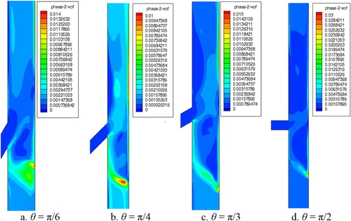
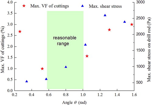
The curves obtained by extracting the data along the vertical path crossing the concentration region reveal that the fluctuations of the VF of the cuttings around the injection nozzle in the joint flow along the path of movement (Figure 22). The vortex underneath the nozzle causes local cuttings concentrations (peaks of the curves in Figure 22) whose values of VF can reach as much as 12 times the inlet value (0.2%). Beyond the joint region (−0.07 m < Y < 0.25 m), the distributions of the cuttings tend to be even. The maximum values of the VF of the cuttings from Figure 22 and the shear stress from Figure 20 are used as the basis for optimizing the injection angle, which is explicated in Figure 23. Influenced by the vortexes in the annulus space, the maximum VF first lowers and then rises with increases in θ, which means there is an optimal region of θ for a lower VF. Taking the shear stress into account, which is better controlled at a low value, θ = 40° ± 10° is proposed as the most reasonable range for the assisted circulation.

Figure 22. VF of the cuttings along the drill pipe.

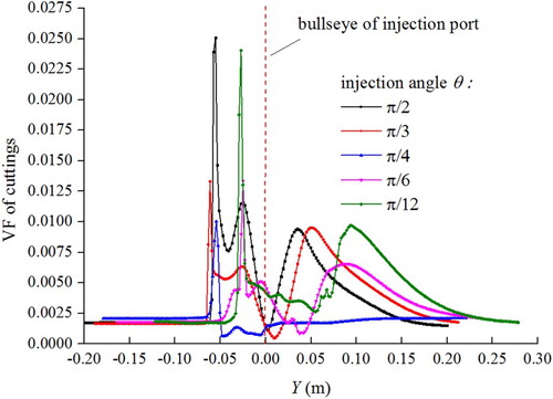
Figure 23. Maximum VF of the cuttings under different injection angles θ.

6. Engineering applications

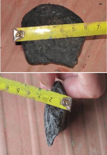
The simulations carried out in this study provide theoretical reference for site operation. When relevant results like using a low-viscosity fluid for assisted circulation and determining the reasonable range for the angle of the injection nozzle are obtained, engineering adjustments can be adopted. Figure 24 shows the equipment and tools for a DCS used at a CBM drilling site. The injection nozzles, connector, and packer are placed at depths of 780.90∼782.28, 805.36, and 785.53∼797.21 m, respectively. The FAC and FMC are set to 14 and 15 l/s, respectively. From the feedback, the DCS possesses a stronger capability for carrying cuttings and keeping the wellbore clear. Figure 25 shows a large cuttings piece removed from the well with dimensions of 60 × 45 × 23 mm, which is never produced in common drilling operations. Moreover, with the DCS, the drilling rate can be increased safely.

Figure 24. Equipment for the double-circulation system (DCS).

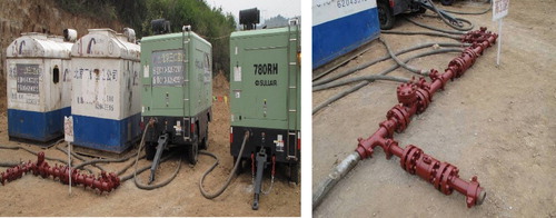
Figure 25. Large cutting removed from Well ZS-3H.

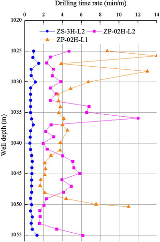
In Figure 26, the drilling rates for Well ZS-3H and the lateral wells in Well ZP-02H (a common drilling operation without using a DCS) in the same depth range (1025∼1055 m) are compared. It can be seen that the drilling in Well ZP-02H is much slower than that in Well ZS-3H, and that there are far more fluctuations in the former, which signifies more uncertainties that threaten the safety and stability of the well drilling operation. In contrast, a steady, high drilling rate (low drilling time) in Well ZS-3H makes for a much more stable and efficient drilling operation.

Figure 26. Drilling rates in wells ZS-3H and ZP-02H.

7. Conclusions

The CFD-DEM coupled model used in this work has been shown to accurately simulate a DCS used for CBM well drilling. The working mechanism and the influences of different parameters have been explored, and the results generated from the simulations have validated the positive impact that the FAC has on cuttings transport in the well annulus. Some recommendations have been arisen from the simulations: (1) verification cases show that flaky particles behave more like the real cuttings particles from a CBM well than spherical particles and better suited for use in the simulations; (2) The application of a DCS can much improve the cuttings transport especially in the curved and horizontal parts of the well even when larger cuttings particles exist; (3) not much difference has been shown in performance to the increasing viscosity of the fluid in a DCS and therefore a low-viscosity fluid is recommended for the DCS; (4) by investigating the VF of the cuttings around the injection nozzles and the shear stress on the wall of drill rod, a reasonable range of 30∼50° for the angle of the injection nozzle is yielded.

However, the study is not without its limitations. The flaky appearance of the cuttings particles may only be suited to simulating cuttings in a CBM well, and improvements to the methodologies adopted for building a non-spherical particle are needed, since deviations still exist when a non-spherical particle is represented by a multi-sphere construct. Therefore, more work is needed in order to refine and further explore this important area of research.

Acronyms

CBM	=	coalbed methane
CDV	=	critical deposition velocity
CFD	=	computational fluid dynamics
CFV	=	critical fluid velocity
CRV	=	critical re-suspension velocity
DCS	=	double-circulation system
DEM	=	discrete element method
FAC	=	flow of assisted circulation
FMC	=	flow of main circulation
PDC	=	polycrystalline diamond compact
UBD	=	underbalanced drilling
VF	=	volume fraction

Disclosure statement

No potential conflict of interest was reported by the authors.

Additional information

Funding

This work was supported by the China Postdoctoral Science Foundation [grant no. 2018M640665] and the National Natural Science Foundation of China [grant nos. 51804330 and 51875579].

References

- Akbarian, E., Najafi, B., Jafari, M., Ardabili, S. F., Shamshirband, S., & Chau, K. W. (2018). Experimental and computational fluid dynamics-based numerical simulation of using natural gas in a dual-fueled diesel engine. Engineering Applications of Computational Fluid Mechanics, 12(1), 517–534.
- Akhshik, S., Behzad, M., & Rajabi, M. (2015). CFD–DEM approach to investigate the effect of drill pipe rotation on cuttings transport behavior. Journal of Petroleum Science and Engineering, 127, 229–244.
- Akhshik, S., & Rajabi, M. (2018). CFD-DEM modeling of cuttings transport in underbalanced drilling considering aerated mud effects and downhole conditions. Journal of Petroleum Science and Engineering, 160, 229–246.
- Alexandrou, A. N., Menn, P. L., Georgiou, G., & Entov, V. (2003). Flow instabilities of Herschel–Bulkley fluids. Journal of Non-Newtonian Fluid Mechanics, 116(1), 19–32.
- Capo, J., Yu, M., Miska, S., Takach, N. E., & Ahmed, R. (2006). Particles transport with aqueous foam at intermediate inclined wells. SPE Drilling & Completion, 21(2), 99–107.
- Carlos Varas, A. E., Peters, E. A. J. F., & Kuipers, J. A. M. (2017). CFD-DEM simulations and experimental validation of clustering phenomena and riser hydrodynamics. Chemical Engineering Science, 169, 246–258.
- Chen, Z., Ahmed, R. M., Miska, S., Takach, N. E., Yu, M., Pickell, M. B., & Hallman, J. (2007). Experimental study on cuttings transport with foam under simulated horizontal Downhole conditions. SPE Drilling & Completion, 22(4), 304–312.
- Chien, S. F. (1994). Settling velocity of irregularly shaped particles. SPE Drilling & Completion, 9(4), 281–289.
- Di Renzo, A., & Di Maio, F. P. (2004). Comparison of contact-force models for the simulation of collisions in DEM-based granular flow codes. Chemical Engineering Science, 59, 525–541.
- Duan, M., Miska, S., Yu, M., Takach, N., & Ahmed, R. (2007). Critical conditions for effective sand-sized solids transport in horizontal and high-angle wells. SPE106707 presented at the Production and Operations Symposium, Oklahoma City, OK.
- Ford, J. T., Peden, J. M., Oyeneyin, M. B., Gao, E., & Zarrough, R. (1990). Experimental investigation of drilled cuttings transport in inclined boreholes. SPE 20421 presented at the 65th Annual Technical Conference and Exhibition of the Society of Petroleum Engineers, New Orleans, LA.
- Ghalandari, M., Koohshahi, E. M., Mohamadian, F., Shamshirband, S., & Chau, K. W. (2019). Numerical simulation of nanofluid flow inside a root canal. Engineering Applications of Computational Fluid Mechanics, 13(1), 254–264.
- Guo, B., Yao, Y., & Ai, C. (2008). Liquid carrying capacity of gas in underbalanced drilling. SPE Western Regional and Pacific Section AAPG Joint Meeting, Bakersfield, CA.
- He, Y., Bayly, A. E., & Hassanpour, A. (2018). Coupling CFD-DEM with dynamic meshing: A new approach for fluid-structure interaction in particle-fluid flows. Powder Technology, 325, 620–631.
- Issakhov, A., Bulgakov, R., & Zhandaulet, Y. (2019). Numerical simulation of the dynamics of particle motion with different sizes. Engineering Applications of Computational Fluid Mechanics, 13(1), 1–25.
- Kelessidis, V. C., & Bandelis, G. E. (2004). Flow patterns and minimum suspension velocity for efficient cuttings transport in horizontal and deviated wells in coiled-tubing drilling. SPE Drilling & Completion, 19(4), 213–227.
- Kloss, C., Goniva, C., Hager, A., Amberger, S., & Pirker, S. (2012). Models, algorithms and validation for opensource DEM and CFD-DEM. Progress in Computational Fluid Dynamics, An International Journal, 12(2/3), 140–152.
- Kruggel-Emden, H., Rickelt, S., Wirtz, S., & Scherer, V. (2008). A study on the validity of the multi-sphere discrete element method. Powder Technology, 188, 153–165.
- Li, X., Li, G., Song, W., Cui, G., Chen, J., & Tang, B. (2013). Research on hole cleaning in horizontal well with aerated underbalanced drilling. Science Technology and Engineering, 13(24), 7138–7142.
- LIGGGHTS. (2011). LAMMPS improved for general granular and granular heat transfer simulations. Retrieved from http://www.liggghts.com
- Liu, D., Bu, C., & Chen, X. (2013). Development and test of CFD–DEM model for complex geometry: A coupling algorithm for Fluent and DEM. Computers and Chemical Engineering, 58, 260–268.
- Manzar, M. A., & Shah, S. N. (2009). Particle distribution and erosion during the flow of Newtonian and Non-Newtonian slurries in straight and coiled pipes. Engineering Applications of Computational Fluid Mechanics, 3(3), 296–320.
- Mei, R. (1992). An approximate expression for the shear lift force on a spherical particle at finite reynolds number. International Journal of Multiphase Flow, 18(1), 145–147.
- Mykytiw, C. G., Davidson, I. A., Shell UBD Global Implementation Team, Frink, P. J., & Blade Energy Partners. (2003). Design and operational considerations to maintain underbalanced conditions with concentric casing injection. IADC/SPE Underbalanced Technology Conference and Exhibition, San Antonio, TX.
- Nguyen, C., Somerville, J. M., & Smart, B. G. D. (2009). Predicting the production capacity during underbalanced-drilling operations in Vietnam. IADC/SPE Managed Pressure Drilling and Underbalanced Operations Conference and Exhibition, San Antonio, TX.
- OpenCFD Ltd. (2009). OpenFOAM – The open source CFD toolbox. Retrieved from http://www.openfoam.com
- Ozbayoglu, E. M., Erge, O., & Ozbayoglu, M. A. (2018). Predicting the pressure losses while the drillstring is buckled and rotating using artificial intelligence methods. Journal of Natural Gas Science and Engineering, 56, 72–80.
- Ozbayoglu, E. M., Saasen, A., Sorgun, M., & Svanes, K. (2010). Critical fluid velocities for removing cuttings bed inside horizontal and deviated wells. Petroleum Science and Technology, 28(1), 594–602.
- Paredes, J. C. B., Lupo, C. P. M., Escalera, H. M., Medina, L. D., Duno, H., Zapata, J. F. G., … Rodriguez, E. J. (2010). Understanding multiphase flow modeling for N2 concentric nitrogen injection through downhole pressure sensor data measurements while drilling MPD wells. SPE/IADC Managed Pressure Drilling and Underbalanced Operations Conference and Exhibition, Kuala Lumpur, Malaysia.
- Saffman, P. G. (1965). The lift on a small sphere in a slow shear flow. Journal of Fluid Mechanics, 22(1), 385–400.
- Sanchez, R. A., Azar, J. J., & Bassal, A. A. (1999). Effect of drillpipe rotation on hole cleaning during directional-well drilling. SPE Journal, 4(2), 101–108.
- Shao, B., Liu, G. R., Lin, T., Xu, G. X., & Yan, X. Z. (2017). Rotation and orientation of irregular particles in viscous fluids using the gradient smoothed method (GSM). Engineering Applications of Computational Fluid Mechanics, 11(1), 557–575.
- Shook, C. A., & Roco, M. C. (1991). Slurry flow: Principles and practice (3rd ed.). Boston, MA: Butterworth-Heinemann.
- Sommerfeld, M. (2000). Theoretical and experimental modelling of particulate flows. Technical Report Lecture Series. von Karman Institute for Fluid Dynamics, 20–23.
- Song, X., Guan, Z., & Chen, S. (2009). Mechanics model of critical annular velocity for cuttings transport in deviated well. Journal of China University Petroleum, 33(1), 53–56.
- Suryanarayana, P. V., Hasan, A. B. M. K., & Hughes, W. J. (2004). Technical feasibility and applicability of a concentric jet pump in underbalanced drilling. SPE/IADC Underbalanced Technology Conference and Exhibition, Houston, TX.
- Tomren, P. H., Iyoho, A. W., & Azar, J. J. (1986). Experimental study of cuttings transport in directional wells. SPE Drilling Engineering, 1(1), 43–56.
- Yang, Y., Cui, S., Wang, F., Zhang, B., Ni, Y., Shen, J., … Liu, S. (2017). Double casing & binary circulation hole cleaning technology for CBM multi-branch horizontal wells. Natural Gas Industry, 37(1), 112–118.
- Yang, Y., Shao, B., Wang, F., Yan, X., Ni, Y., Cui, S., & Yang, Y. (2015). Dynamic crushing mechanism of well-wall in engraving stage of sidetracking based on Lagrange explicit algorithm. Journal of China Coal Society, 40(7), 1491–1497.
- Zeng, J., Li, H., & Zhang, D. (2016). Numerical simulation of proppant transport in hydraulic fracture with the upscaling CFD-DEM method. Journal of Natural Gas Science and Engineering, 33, 264–277.
- Zhao, J., & Shan, T. (2013). Coupled CFD-DEM simulation of fluid-particle interaction in geomechanics. Powder Technology, 239, 248–258.
- Zhong, W., Yu, A., Liu, X., Tong, Z., & Zhang, H. (2016). DEM/CFD-DEM modelling of non-spherical particulate systems: Theoretical developments and applications. Powder Technology, 302, 108–152.
- Zhu, X., Liu, S., & Tong, H. (2011). Research on transport of cuttings in gas drilling horizontal well and cuttings falling-prevent joint development. SPE Asia Pacific Oil and Gas Conference and Exhibition, Jakarta, Indonesia.