Multi-objective optimization and comparison of surrogate models for separation performances of cyclone separator based on CFD, RSM, GMDH-neural network, back propagation-ANN and genetic algorithm

Abstract

Pressure drop (Δp) and collection efficiency (η) are used to evaluate the separation performance of the cyclone separator. In this study, we conducted comparative study of cyclone models using response surface methodology (RSM), back propagation neural network (BPNN), and group method of data handling (GMDH) networks to develop optimal predictive cyclone models. Also, we conducted multi-objective optimization for maximizing model and minimizing model using genetic algorithm (GA). CFD was performed instead of experimental method to get the estimated values for modeling of Δp and η. The validation results of CFD showed 0.5% and 2% errors for Δp and η, respectively, compared with the experimental data. Second, design of experiment (DOE) analysis for 10 cyclone geometrical parameters was executed to obtain the significant geometrical parameters. Vortex finder diameter D_x, inlet width a, inlet height b and cone height H_co have a significant effect on η and Δp. However, interaction effects between the geometrical parameters have small effects. The cyclone models by RSM, BPNN and GMDH based on 25 CFD training set were developed. The predictive performance results by the cyclone models were compared by 25 CFD test set. The GMDH method achieved the best prediction for Δp ($R^2=99.7$, RMSE = 0.102) $R_{\text{adjusted}}^2=98.99$, RMSE = 0.0119) than the RSM, BPNN cyclone models. Additionally, uncertainty analysis was performed to estimate the quantitative performance of cyclone models. The results show that the uncertainty width of GMDH models achieved the best prediction ($\eta$: ±0.0065, Δp: ±0.0188). Finally, GA was applied to optimize the GMDH models simultaneously. GA generated 70 non-dominant solutions. Reproducibility of five optimal points was validated by using CFD. The trade-off optimal point showed improvement by 24.31%, 18% and 8.79% for Δp ${\text{d}}_{50}$ and $\eta$, respectively.

KEYWORDS:

• Cyclone separator
• Computational Fluid Dynamics (CFD)
• Response Surface Methodology (RSM)
• Artificial Neural Network (ANN)
• Genetic Algorithm (GA)
• Multi-objective optimization

1. Introduction

1.1. Research background

In many industries, the contaminants are removed using various dust collectors. In comparison with other type of dust collectors, such as settling chamber, wet scrubbers and electrostatic precipitators etc., gas–solid cyclone separator using a centrifugal force were widely used in industrial processes due to the advantages of its relatively low maintenance cost, simple structure and robustness of operating conditions under high temperature and pressure (Hoffmann & Stein, 2008). Pressure drop ‘Δp’ (also expressed as Euler number) and collection efficiency ‘η’ (also known as the separation efficiency and cut-off diameter) are used to evaluate the separation performance of the cyclone separator. The cut-off diameter is a particle diameter for which η is 50% and Euler number is the dimensionless measure of the pressure drop. The performance parameters are defined as follow; (1) $\eta =1-\frac{{\text{N}}_{\text{out}}\left(\text{d}\right)}{{\text{N}}_{\text{in}}\left(\text{d}\right)}$(1) Where ${\text{N}}_{\text{in}}$ is the total number of particles, and ${\text{N}}_{\text{out}}$ is the total number of particles discharged in the cyclone vortex finder. 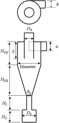(2) $\mathrm{\Delta }P=P_{\text{in}}-P_{\text{out}}$(2) Where $P_{\text{in}}$ is the pressure in the cyclone inlet, and $P_{\text{out}}$ is the pressure in the cyclone outlet. The performance parameters are closely dependent of the geometric parameters of cyclone. The configuration and nomenclature of 10 geometric parameters of cyclone is shown in Figure 1. Ten parameters are diameter of vortex finder ${\text{D}}_{\mathrm{x}}$, inlet height$\text{a}$, inlet width $\text{b}$, cylinder height ${\text{H}}_{\text{cy}}$, cone height ${\text{H}}_{\text{co}}$, cone tip diameter ${\text{B}}_{\mathrm{c}}$, tube height ${\text{H}}_{\mathrm{t}}$, collector height ${\text{H}}_{\mathrm{c}}$ and collector diameter ${\text{D}}_{\mathrm{c}}$, vortex finder length $\text{S}$.

Figure 1. Geometry and nomenclature of 10 geometric parameters of cyclone.

Generally, as Δp increases, η also increases. However, the optimal cyclone should be designed to have minimum Δp and maximum η. Therefore, many studies have been reported for several decades to model and optimize the performance parameters according to the geometric parameters of cyclone.

Early researches developed empirical models for Δp and η according to massive experiments and mathematical equations (Avci & Karagoz, 2001; Barth, 1956; Dietz, 1981; Leith, 1990; Muschelknautz & Krambrock, 1970; Shephered & Lapple, 2005). The empirical model was developed by conservation law's equation and experimental data. Gimbun, Chuah, Choong, and Fakhru’l-Razi (2005) showed by comparing the CFD results with the cyclone performances predicted from the various empirical models.

With the advance of high-performance computers and CFD technology, CFD has been considered as another approach to optimize Δp and η recently. CFD have advantages of time saving and high accuracy as well as the ability to calculate physical quantities that are difficult to be measured experimentally (Elsayed & Lacor, 2012). Therefore, many CFD studies have been performed for optimizing Δp and η depending on the geometrical parameters. The effects of pressure drop and collection efficiency on the changes of the cyclone vortex finder shape were investigated using CFD (De Souza, Salvo, & Martins, 2015; Raoufi, Shams, Farzaneh, & Ebrahimi, 2008). The CFD simulation of cyclone flow was performed according to changing the cyclone inlet shape (Bernardo, Mori, Peres, & Dionísio, 2006; Elsayed & Lacor, 2011; Yang, Sun, & Gao, 2013). The cyclone performance parameters were investigated according to changing the cyclone body shape (Brar, Sharma, & Elsayed, 2015; Hamdy, Bassily, El-Batsh, & Mekhail, 2017; Safikhani, Akhavan-Behabadi, Shams, & Rahimyan, 2010). The cyclone flow was investigated by changing the cyclone dust collector shape (Ganegama Bogodage & Leung, 2015; Kaya & Karagoz, 2009; Qian, Zhang, & Zhang, 2006). These studies performed by changing only one geometrical parameter and others were fixed. This did not consider the interactive effect among the geometric parameters. This brings about local optimization.

Recently, ANN techniques and GA method has been successfully applied to many industries (Ardabili et al., 2018; Ebtehaj & Bonakdari, 2016; Fotovatikhah et al., 2018; Gholami et al., 2018; Moazenzadeh, Mohammadi, Shamshirband, & Chau, 2018; Najafi, Faizollahzadeh Ardabili, Shamshirband, Chau, & Rabczuk, 2018; Taherei Ghazvinei et al., 2018). Also, cyclone optimization studies have been performed by combing Design of Experiment (DOE) with various modeling methods such as Response Surface Methodology (RSM) and Artificial Neural Network (ANN) methods. A number of optimization studies are relatively limited, compared to the experiment and simulation studies (Sun & Yoon, 2018).

Elsayed and Lacor (2012) conducted a multi-objective optimization study for seven geometrical parameters using non-dominated sorting genetic algorithm (NSGA-II). They obtained the radial basis function neural network (RBFNN) models for Euler number (Δp) and cut-off diameter (η) based on results of the empirical model. The empirical models can yield the estimated values faster than using CFD. However it is not suitable for cyclonic optimization because the predictive performance of empirical model is less accurate for complex geometry.

Sun, Kim, Yang, Kim, and Yoon (2017) conducted multi-objective optimization for Δp and η based on CFD, the desirability function method and response surface method (RSM). As optimization results, Δp and η were improved by 20.7% and 24.2%, respectively, compared to the reference model. Also, Sun and Yoon (2018) added the cyclone surface roughness as a new design variable and increased the level range of the existing design variables and optimized it by using NSGA-II. However, it was found that cited reference values of Δp and η are significantly different at the optimization study using NSGA-II. Therefore, a reasonable comparison of optimization results cannot be taken ahead.

Khalkhali and Safikhani (2012) developed the models of Δp and η according to the four cyclone geometric parameters based on CFD and GMDH neural network. The developed cyclone models were optimized simultaneously using NSGA-II. Multi-objective optimization was executed based on the NSGA-II. However, the reproducibility of the optimized results was not confirmed by CFD simulations. This cannot confirm the proper optimization results.

Elsayed and Lacor (2013) optimized the four geometric parameters of the Stairmand design cyclone using CFD, RSM and desirability functions. The new design has achieved high performance. However, the errors between RSM results and CFD results for Δp and η were 17.20% and 20.23%, respectively. In addition, a cyclone performance models were developed using RBFNN as an alternative to RSM. However, the predicted performance of the developed RBFNN model was evaluated quantitatively based on the training data set. That approach might result in over fitting. A different test set should have been used to evaluate the prediction performance of model instead of the training set that used to train the model. In addition, this study did not verify the physical justification for optimized reasons. It cannot explain why the optimized model outperforms than the existing baseline model.

1.2. Study objectives

The objectives of present study are summarized in three:

1. Analysis of effect of significant geometrical parameters out of 10 geometrical parameters on the cyclone performance parameters using DOE analysis with CFD results: The significant geometrical parameters assist to reduce the number of DOE data sets required for surrogate modeling, as well as to solve local optimizations that occur when only one design variable is changed. Previous work of cyclone using CFD overlooks better optimization performance due to local optimization problems (Elsayed & Lacor, 2011; Ganegama Bogodage & Leung, 2015; Raoufi et al., 2008).

2. Development and Comparison of predictive models based on RSM, GMDH technique and BPNN technique for predicting cyclone performance ?>parameter with respect to the cyclone geometric parameters: Each cyclone performance prediction model is compared quantitatively using AIC, R2, RMSE, and R2_adj, and uncertainty analysis is performed on the developed models. To the best of our knowledge, there are no studies comparing simultaneously the predictive performance of Δp and η models obtained by using the various ANN methodologies and the RSM using the same training dataset and test dataset in many cyclone studies.

3. Multi-objective optimization of the cyclone models that have the best predictive performance using NSGA-II: The optimized results compare not only the improvement of the cyclone performance models (Δp, η) with the reference model, but also analyze from the viewpoint of physical justification of the optimization result. The limitations of previous optimization researches lack an analysis of why the optimization was made (Elsayed & Lacor, 2013; Khalkhali & Safikhani, 2012).

1.3. Reference model: Muschelknautz method of modeling

For this optimization study, Muschelknautz method (MM) of modeling (Muschelknautz & Krambrock, 1970) was selected as a reference model because it contains the shape of the cyclone dust collector as a design parameter, compared to the other cyclone mathematic model, and many experimental results (Obermair & Staudinger, 2001; Obermair, Woisetschläger, & Staudinger, 2003) are available for CFD validation. The reference model will be compared to the optimized cyclone model. The 10 geometric parameters and geometric ratio of the MM model presents in Table 1.

Table 1. Geometrical parameters values for Obermair et al. (2003). (D = 0.4 m).

Factors	${\displaystyle \frac{{\text{D}}_{\mathrm{x}}}{D}}\left(\text{x}1\right)$	${\displaystyle \frac{\text{a}}{D}}\left(\text{x}2\right)$	${\displaystyle \frac{\text{b}}{D}}\left(x3\right)$	${\displaystyle \frac{Hy}{D}}\left(x1\right)$	${\displaystyle \frac{{\text{H}}_{\text{co}}}{D}}\left(\text{x}5\right)$	${\displaystyle \frac{{\text{B}}_{\mathrm{c}}}{D}}\left(\text{x}6\right)$	${\displaystyle \frac{{\text{H}}_{\mathrm{t}}}{D}}\left(x7\right)$	${\displaystyle \frac{{\text{H}}_{\mathrm{c}}}{D}}\left(\text{x}8\right)$	${\displaystyle \frac{{\text{D}}_{\mathrm{c}}}{D}}\left(\text{x}9\right)$	${\displaystyle \frac{\text{S}}{D}}\left(\text{x}10\right)$
Value	0.375	0.25	0.4375	1.25	1.225	0.225	0.74	0.735	0.375	0.45

1.4. Study outline

The flow chart relationship in this study is shown in Figure 2. This optimization study followed the following steps. First, CFD simulations are performed on the cyclone flow using the turbulence models and the DPM. For time and convenience, CFD is used instead of experimental method to get estimated values for modeling of Δp and η. The CFD results are validated by comparison with experiment results of the reference model available in the literature (Muschelknautz & Krambrock, 1970; Obermair et al., 2003; Obermair & Staudinger, 2001).

Figure 2. The flow-chart relationship of present work.

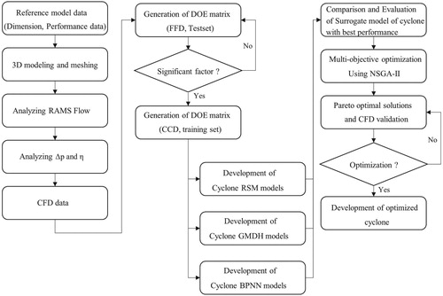
Next, the DOE analysis for the 10 cyclone geometric parameters is performed to get the significant geometric parameters. And then, the models based on RSM, GMDH-NN and BPNN combined with the DOE method have been developed to predict $\eta$ and $\mathrm{\Delta }\text{p}$ with respect to the significant geometric parameters. The prediction performances of the cyclone performance models are compared to analyze the advantages of each methodology and differences between the models. And then, an optimal predictive model for $\eta$ and $\mathrm{\Delta }\text{p}$ is selected.

Finally, the optimal predictive models were simultaneously optimized to get maximum $\eta$ and minimum $\mathrm{\Delta }\text{p}$ using NSGA-II. The ‘trade-off’ solution between optimal models was selected in optimal Pareto front, and the reproducibility was verified by using CFD with the Reynold stress model. The improvement rates of optimized results were compared with the reference model quantitatively.

2. Numerical simulation of cyclone separator

2.1. Reynolds averaged Naiver-Stokes (RANS) for turbulence models

An appropriate turbulence model should be used to simulate the turbulence behavior in CFD. The Reynolds averaged Naiver-Stokes (RANS) turbulence models have been successfully applied to predict the turbulence flow in many industrial applications. Many studies have been conducted on the application of turbulence models to capture the behavior of cyclone flow. Boyan, Ayers, and Swithenbank (1982) found the $k-\epsilon$ models cannot predict the turbulence behavior of cyclone with significant non-equilibrium effects of turbulent transport. Qian et al. (2006) showed that the cyclone flow can capture using the Reynold stress model (RSM) which assumes a Reynolds stress tensor with isotropic eddy-viscosity hypothesis. In addition to the RANS model, LES (Large Eddy Simulation) shows relatively better prediction results about the cyclone than RSM, but LES requires computational resources several times larger than RSM (Elsayed & Lacor, 2013). Therefore, in this study, the RSM was used to simulate the cyclone flow. The RSM are expressed as follow: (3) $\begin{array}{rl}& \frac{\mathrm{\partial }}{\mathrm{\partial }\text{t}}{\text{R}}_{\text{ij}}+{\overline{u}}_k\frac{\mathrm{\partial }}{\mathrm{\partial }{x}_{\mathrm{k}}}{\text{R}}_{\text{ij}}={\text{D}}_{\text{Tij}}+{\text{P}}_{\text{ij}}+{\text{F}}_{\text{ij}}+{\mathrm{\Phi }}_{\text{ij}}-{\epsilon }_{\text{ij}}\end{array}$(3) (4) $\begin{array}{rl}& {\text{D}}_{\text{T,ij}}\left(\text{turbulent diffusion}\right)\\ & =-\frac{\mathrm{\partial }}{\mathrm{\partial }{\text{x}}_{\mathrm{k}}}[\rho \overline{{{\text{u}}^{\mathrm{\prime }}}_{\mathrm{i}}{{\text{u}}^{\mathrm{\prime }}}_{\mathrm{j}}{{\text{u}}^{\mathrm{\prime }}}_{\mathrm{k}}}+\rho \left({\delta }_{\text{kj}}{{\text{u}}^{\mathrm{\prime }}}_{\mathrm{i}}+{\delta }_{\text{ik}}{{\text{u}}^{\mathrm{\prime }}}_{\mathrm{j}}\right)\end{array}$(4) (5) $\begin{array}{rl}& {\text{P}}_{\text{ij}}\left(\text{stress production}\right)=-\rho \left(\overline{{{\text{u}}^{\mathrm{\prime }}}_{\mathrm{i}}{{\text{u}}^{\mathrm{\prime }}}_{\mathrm{k}}}\frac{\mathrm{\partial }{\text{u}}_{\mathrm{j}}}{\mathrm{\partial }{\text{x}}_{\mathrm{k}}}+\overline{{{\text{u}}^{\mathrm{\prime }}}_{\mathrm{i}}{{\text{u}}^{\mathrm{\prime }}}_{\mathrm{k}}}\frac{\mathrm{\partial }{\text{u}}_{\mathrm{i}}}{\mathrm{\partial }{\text{x}}_{\mathrm{k}}}\right)\end{array}$(5) (6) $\begin{array}{rl}& {\text{F}}_{\text{ij}}\left(\text{rotation production}\right)\\ & =-\text{2}\rho {\mathrm{\Omega }}_{\mathrm{k}}\left(\overline{{{\text{u}}^{\mathrm{\prime }}}_{\mathrm{j}}{{\text{u}}^{\mathrm{\prime }}}_{\mathrm{m}}}{\epsilon }_{\text{ikm}}+\overline{{{\text{u}}^{\mathrm{\prime }}}_{\mathrm{i}}{{\text{u}}^{\mathrm{\prime }}}_{\mathrm{k}}}{\epsilon }_{\text{jkm}}\right)\end{array}$(6) (7) $\begin{array}{rl}& {\mathrm{\Phi }}_{\text{ij}}\left(\text{pressure strain}\right)=-\text{p}\left(\frac{\overline{\mathrm{\partial }{{\text{u}}^{\mathrm{\prime }}}_{\mathrm{i}}}}{\mathrm{\partial }{\text{x}}_{\mathrm{j}}}+\frac{\overline{\mathrm{\partial }{{\text{u}}^{\mathrm{\prime }}}_{\mathrm{j}}}}{\mathrm{\partial }{\text{x}}_{\mathrm{i}}}\right)\end{array}$(7) (8) $\begin{array}{rl}& {\epsilon }_{\text{ij}}\left(\text{pressure strain}\right)=-\text{2}\mu \left(\frac{\overline{\mathrm{\partial }{{\text{u}}^{\mathrm{\prime }}}_{\mathrm{i}}}}{\mathrm{\partial }{\text{x}}_{\mathrm{k}}}\frac{\overline{\mathrm{\partial }{{\text{u}}^{\mathrm{\prime }}}_{\mathrm{j}}}}{\mathrm{\partial }{\text{x}}_{\mathrm{k}}}\right)\end{array}$(8) where $\text{p}$ and $\mu$ are, respectively, pressure, the molecular viscosity, and $\delta$ is Kronecker delta.

2.2. Discrete phase models (DPM)

The particle trajectory in cyclone was calculated by Lagrangian-based discrete phase model (DPM). The DPM assumes that the particle phase does not affect the continuous phase when the volume occupied by the particles in the continuous phase was less than 10% in DPM (ANSYS FLUENT, 2016). So, DPM can be applied in cyclone simulation. Transport momentum equation for each particle is expressed as: (9) $\frac{d{\overrightarrow{\mathrm{u}}}_{\mathrm{p}}}{\text{dt}}={\text{F}}_{\mathrm{D}}\left({\overrightarrow{\mathrm{u}}}_k+u_k^{\mathrm{\prime }}-{\overrightarrow{\mathrm{u}}}_{\mathrm{p}}\right)+\frac{\overrightarrow{\mathrm{g}(}{\rho }_{\mathrm{p}}-\rho )}{{\rho }_{\mathrm{p}}}+\text{F}$(9) where the term ${\text{F}}_{\mathrm{D}}\left({\overrightarrow{\mathrm{u}}}_{\mathrm{k}}+u_k^{\mathrm{\prime }}-{\overrightarrow{\mathrm{u}}}_{\mathrm{p}}\right)$ is the drag force per unit particle mass, ${\overrightarrow{\mathrm{u}}}_{\mathrm{k}}$ is the time-averaged fluid velocity in the k-th direction obtained by solving the RANS model, $u_k^{\mathrm{\prime }}$ is the instantaneous fluctuation velocity in the k-th direction and $\text{F}$ is an additional acceleration (force/unit particle mass), ${\rho }_{\mathrm{p}}$, $\rho$ are the particle density and the flow density, respectively. The drag force and drag coefficient of the spherical particles is calculated as (10) $\begin{array}{rl}{\text{F}}_{\mathrm{D}}& =\frac{18\mu }{{\rho }_{\mathrm{p}}{d}_{\mathrm{p}}^{\text{2}}}\frac{{\text{C}}_{\mathrm{D}}\text{R}{\text{e}}_{\mathrm{p}}}{\text{24}}\end{array}$(10) (11) $\begin{array}{rl}{C}_{\mathrm{D}}& =\left\{\begin{array}{ll}\frac{24}{\text{Re}}& \text{R}{\text{e}}_{\mathrm{p}}\le 1,\\ \frac{24(1+{\text{0.15Re}}_{\mathrm{p}}^{0.687})}{\text{R}{\text{e}}_{\mathrm{p}}}& 1<\text{R}{\text{e}}_{\mathrm{p}}\le 1000,\\ 0.44& 1000<\text{R}{\text{e}}_{\mathrm{p}},\end{array}\right.\end{array}$(11) where the term ${\text{C}}_{\mathrm{D}}$ is drag coefficient of the spherical particle, $\text{R}{\text{e}}_{\mathrm{p}}$ is the particle Reynold number. The turbulence fluctuations are random functions of space and time. A discrete random walk (DRW) model is applied to simulate the instantaneous fluctuation velocity ($u_k^{\mathrm{\prime }}$) in this study. The $u_k^{\mathrm{\prime }}$ affects to the particle transport for small particles. The values of $u_k^{\mathrm{\prime }}$ that prevail during the lifetime of the turbulent eddy are sampled by assuming that they obey a Gaussian probability distribution as (ANSYS FLUENT, 2016). (12) $u_k^{\mathrm{\prime }}=\xi \sqrt{\overline{u_k^{\mathrm{\prime }}{u}_k^{\mathrm{\prime }}}}$(12) Where, $\xi$ is a normally distributed random number. $\overline{u_k^{\mathrm{\prime }}{u}_k^{\mathrm{\prime }}}$ is the local RMS value of the velocity fluctuations. The characteristic lifetime of the eddy (${\tau }_{\mathrm{e}}$) is defined either as a constant given by: (13) ${\tau }_{\mathrm{e}}=2{\text{T}}_{\mathrm{L}}$(13) where ${\text{T}}_{\mathrm{L}}$ is the eddy turn over time given as, ${\tau }_{\mathrm{e}}=0.3\text{k}/\text{e}$. The other option allows for a long–normal random variation of eddy lifetime that is given by: (14) ${\tau }_{\mathrm{e}}=-{\text{T}}_{\mathrm{L}}\text{log}\left(r\right)$(14) where r is a uniform random number between 0 and 1. The option of random calculation of ${\tau }_{\mathrm{e}}$ yields a more realistic description of the correlation function.

2.3. CFD simulation setup

Since cyclone flows have the characteristics of strong vortex and steep pressure distribution, it is necessary to accurately predict cyclone flows using powerful and efficient algorithms. Shukla, Shukla, and Ghosh (2011) conducted a case study to select the optimal algorithm that can accurately simulate the cyclone flow. According to the results of the case study, in this study, the velocity and pressure was connected by SIMPLE algorithm, for static pressure distribution and the pressure drop, it was interporated by the PRESTO method. Advection terms were discretized by using the QUICK. The second-order upwind scheme was used for the momentum, turbulence dissipation rates and turbulence kinetic energy. To reduce the numerical instability and to improve convergence, the first-order upwind scheme was used for the Reynolds stress.

The boundary conditions in this study were identical to the conditions used in the reference model. The cyclone inlet was set to uniform velocity and the air flow rate is 800 m³/h (12.7 m/s). The cyclone outlet was set to atmospheric pressure. The cyclone wall was set to no-slip conditions. For the convergence of the cyclone flow, the convergence criteria for optimization process are until there is no fluctuation of pressure drop. The all simulation are conducted as follow, First, the steady-state solution reached 3,000 iterations for stability of the solution. And then, the iteration number per time step and the time step size were selected as 1500 and 0.001 s, respectively. This creates a physical time of 1.5 s. The boundary conditions for the CFD simulation were listed in Table 2. The commercial FVM simulation software ANSYS Fluent 16.2.was used to simulate the cyclone performance parameters.

Table 2. Boundary condition for the cyclone CFD simulation.

Inlet velocity	12.69 (m/s)
Pressure outlet	101325 (Pa)
Wall	No slip condition
Air viscosity	1.82 × 10−5 N × m^2
Air density	1.203 kg
Time step size	0.001 s
Iteration number per time step	1500

2.4. DPM setting

For the discrete phase modeling (DPM) condition, the collusion condition between the wall and the particles was selected as elastic conditions. The collection of particles is calculated if the particles reach the dust collector bottom. The particles density is 2770 kg/m³. The number of injected particles is 10⁴ in the all simulation. The particle size distribution is divided to 10 class based on the Rosin-Rammler theory (ANSYS FLUENT, 2016). (15) $Y_d=e^{-{\left(d/\overline{d}\right)}^n}$(15) Where the n is the diffusion parameter. The d is the mean diameter. For simulation, the d, n is defined to 5 µm and 3.5, respectively. Also, the distribution of particle diameters is set from 1 to 10 µm. The particles are divided into 10 classes. So, the particles can be mixed sufficiently. The injected 10⁴particles are tracked to calculate the collection efficiency of the cyclone about all simulation.

2.5. Comparison between CFD results and reference model

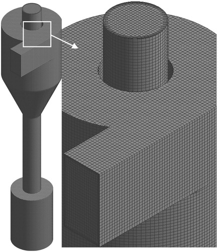
2.5.1. CFD grid independence test

As the grid density is increased, the precise solution could be obtained. However, as the number of grid increases, the CPU time also increases. Figure 3 shows grid for cyclone generated by using cut-cell meshing of ANSYS Meshing 16.1. The geometric ratio of cyclone was used as the reference model. The near-wall treatment was achieved by using scalable wall functions considering the grid refinement with y⁺ < 11 (ANSYS FLUENT, 2016).

Figure 3. Mesh for the simulation of the cyclone.

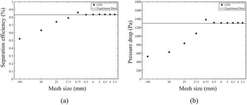
In this study, the grid independence test was conducted until $\eta$ and $\mathrm{\Delta }\text{p}$ were converged according to increasing the grid edge size. Figure 4 presents that the results of grid test for $\eta$ (cf. Figure 4(a)) and $\mathrm{\Delta }\text{p}$ (cf. Figure 4(b)). It showed that the $\mathrm{\Delta }\text{p}$ and $\eta$ converged at the 6.5 mm of maximum grid size. Thus, in the all simulation, the maximum grid of 6.5 mm was used.

Figure 4. (a) Results of the mesh independence test of the separation efficiency. (b) Result of the mesh independence test of the pressure drop.

Note: unit % is multiplied by 100.

2.5.2. Validation of results for velocity distribution

To validate the CFD simulation of cyclone, CFD simulation of cyclone velocity distribution was compared with the results of available experimental data. Figure 5 presented the consistency between the experimental data using Laser Doppler anemometry (LDA) method (Obermair et al., 2003) and simulated results for tangential and axial velocities at y = 0.75D and y = 0.368D. As shown in Figure 5, The $k-\epsilon$ models cause excessive turbulent viscosities and unrealistic tangential velocities due to the Boussinesq eddy viscosity assumption. 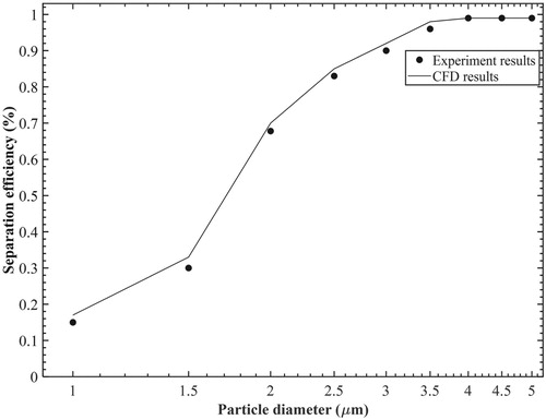Therefore, the $k-\epsilon$ models cannot capture the cyclone flow. Whereas, the Reynolds Stress Model (RSM) can accurately capture the cyclone flow because the RSM assumes a Reynolds stress tensor with three-dimensional anisotropic property (ANSYS FLUENT, 2016). Furthermore, the collection efficiency curve from CFD results was compared with the experimental results in Figure 6. The CFD results were consistent with those obtained experimentally. The error between experiment result and CFD results for $\eta$ and $\mathrm{\Delta }\text{p}$ were 1.1% and 0.5% respectively. Therefore, $\eta$ and $\mathrm{\Delta }\text{p}$ resulted from CFD showed reasonable results by comparing the experiment data. This verified CFD simulation can be reasonably used for various surrogate model method, such as response surface methodology and artificial neural network systems.

Figure 5. Comparison of CFD result for distribution of velocity with experiment data. The three rows present comparison against Moazenzadeh et al. (2018) from left to right: first column – tangential velocity; second column – axial velocity; from top to bottom: axial location in 0.75D (A-A′) and 0.368D (B-B′), respectively.

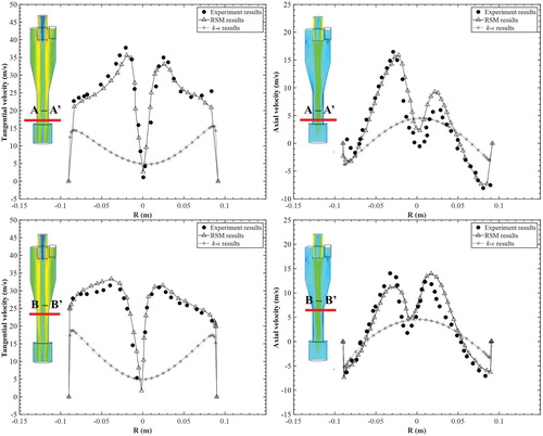
Figure 6. Comparison of CFD result for separation efficiency curve with experiment data Moazenzadeh et al. (2018).

Note: unit % is multiplied by 100.

3. Surrogate model development for $\text{η}$ and $\mathbf{\Delta }\mathbf{\text{p}}$

3.1. Design of experiment

Design of Experiment (DOE) is a systematic method, which can be effectively used to investigate the effect of change of design variables on the response(s) and to provide reasonable answers about the behavior of a system (Mathews, 2005). In particular, the modeling techniques, such as artificial neural networks (ANN) and response surface techniques (RSM), are successfully combined with DOE methods (Khayet, Cojocaru, & Essalhi, 2011; Rahimpour, Hatti-Kaul, & Mamo, 2016). The DOE method can generate a matrix that provides maximum information by minimizing the combination of variables. In general, the fractional factorial design (FFD) method and the central composite design (CCD) method are most commonly used. The DOE method can efficiently apply not only to generate train set for determining the parameters of model but also to generate test set for evaluating the predictive performance of the model.

3.1.1. Fractional factorial design

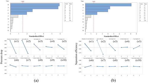
As the number of design variables increases, the number of physical/numerical experiments is increased exponentially to generate the DOE matrix. If a lot of design variables are considered to model ANN and RSM based on DOE, it takes lots of time to obtain the physical/ numerical experiment results. For solving the problem of many variables, fractional factorial design (FFD) method is introduced. It is effective to reduce the number of runs by compounding high-order interaction effects. It is advisable to use the FFD to investigate design variables that have a statistically significant effect before implementing modeling techniques to reduce the experiments size (Sun et al., 2017). Table 3 presents the selected cyclone geometric parameters for the FFD with IV resolution and the corresponding range of levels (−1, +1) (Hoffmann & Stein, 2008). The FFD of IV resolution with 32 CFD runs was performed. The statistical significance for cyclone geometric parameters was analyzed by Pareto chart with analysis of variance (ANOVA).

Table 3. Levels and factors for factorial experiment.

Factor	Min (−1). (X/D)	Ref. (X/D)	Max. (X/D)
$D_x/D$ (x1)	0.275	0.375	0.475
$a/D$ (x2)	0.15	0.25	0.35
b$/D$ (x3)	0.3375	0.4375	0.5375
$H_{cy}/D$ (x4)	0.75	1.25	1.5
$H_{co}/D$ (x5)	0.5	1.225	1.95
$B_{\mathrm{c}}/D$ (x6)	0.3	0.225	0.25
$H_t/D$ (x7)	0.6	0.74	0.8
$H_c/D$ (x8)	0.635	0.735	0.835
$D_c/D$ (x9)	0	0.375	0.75
$S/D$ (x10)	0.3	0.45	0.6

Cyclone diameter: 0.4 m

Figure 7 shows the main effect plot and Pareto chart for $\mathrm{\Delta }\text{p}$ (cf. Figure 7(a)) and $\eta$ (cf. Figure 7(b)) at the α = 0.05 significance level. Higher-order terms are not included in the chart because they have very small effects. Therefore, the higher term has been ignored. The vortex finder diameter D_x(x1), the inlet width a (x2), the inlet height b (x3) and the cone height H_co (x5) have a significant effect on $\eta$ and $\mathrm{\Delta }\text{p}$. Also, the result of the main effects for $\eta$ and $\mathrm{\Delta }\text{p}$ showed the same tendency as Pareto chart results. In the case of the x5, it showed a negative effect on and $\mathrm{\Delta }\text{p}$ and a positive effect on- $\eta$. Therefore, the four geometric parameters (D_x, a,b,H_co) are selected as design parameter for modeling $\mathrm{\Delta }\text{p}$ and $\eta$ at next section. The other parameters are set as average values between minimum and maximum values.

Figure 7. Analysis of design of experiment for the pressure drop (a) and separation efficiency (b); from top to bottom: Pareto chart, main effect plot.

3.2. Response surface methodology (RSM)

RSM uses a strong statistical method based on the least square method that fits of the estimated values obtained from experiment/simulation to the quadratic polynomial model of RSM. In order to predict the system behavior, the quadratic or higher-order polynomial model is applied in many industrial applications. For modeling the cyclone performance parameters according to geometric parameters, the polynomial equation of RSM is expressed as a general form: (16) $y_k={\text{β}}_0+\sum _{\text{i}=1}^4{\text{β}}_{\mathrm{i}}{\text{x}}_{\mathrm{i}}+\sum _{\text{i}=1}^{\text{4}}.\sum _{\text{j}=1}^4{\text{β}}_{\text{ij}}{\text{x}}_{\mathrm{i}}{\text{x}}_{\mathrm{j}}+\sum _{\text{i}=1}^4{\text{β}}_{\text{ii}}{\text{x}}_{\mathrm{i}}^{\text{2}}+\epsilon$(16) where $y_k$ is the response surface models (k = 1 for collection efficiency and k = 2 for pressure drop), and ${\text{x}}_{\mathrm{i}}$ and ${\text{x}}_{\mathrm{j}}$ are the cyclone geometric parameters. ${\text{β}}_0$, ${\text{β}}_{\mathrm{i}}$, ${\text{β}}_{\text{ij}}$, ${\text{β}}_{\text{ii}}$ are the regression coefficients for each constant, linear, interaction, and square term. $\epsilon$ is the prediction error of the model. The regression coefficients were obtained by the ordinary least square (OLS) method. The OLS is represented as follow, (17) ${\text{β}}_{OLS}=({\mathit{X}}^T\mathit{X}{)}^{-1}{\mathit{X}}^T\mathit{Y}$(17) Where ${\text{β}}_{OLS}$ is a regression coefficient vector, X is the matrix about the tested four geometrical parameters. The matrix is generated using DOE method, which includes all combinations of the four geometrical parameters. Y is the column vector of the experiment/simulation results in the DOE matrix. In other words, the main advantage of RSM is that it is simple and fast to develop predictive models, but the nonlinear nature of the model is relatively small compared to ANN.

A typical DOE matrix for obtaining RSM model is the central composite design (CCD) method (Mathews, 2005). The CCD enables to estimate the square terms of the second-order model efficiently. The CCD consists of a factorial experiment point, a center point and an axial point. If the number of the design variables is k, the total number of experiments of CCD can be written as (18) $\text{N}=2^{\mathbf{\text{k}}}+2\text{k}+{\text{n}}_{\mathrm{c}}$(18) where 2^k is the factorial experiment points, and 2k is the axial points, and n_c is the number of iterations at the center point. A value of α depends on the number of experimental results in the factorial experiment point: (19) $\alpha ={\mathbf{2}}^{(k-p)/4}$(19) where if k is 0, that is full factorial design. And if k is constants, that is fractional factorial design, α is the rotatability. All factors are investigated in five levels (−α, −1, 0, 1, +α). In this work, the DOE matrix for CCD is generated by using the statistical analysis program (Minitab 17, MINITAB Inc.).

3.3. Group method of data handling (GMDH) type neural network

The GMDH algorithm pertains to computer-based mathematical modeling techniques. One of the characteristics of GMDH is the fully automatic architecture and parametric optimization of the model (Onwubolu, 2015). The GMDH algorithm consists of several layers containing neurons. Each neuron has two inputs ($x_i$, $x_j$) and on single output (${\hat{y}}_n$). The output of each neuron can be represented through a quadratic polynomial as Eq.20. (20) $\begin{array}{r}{\hat{y}}_n=w_0+w_1{x}_{in}+w_2{x}_{jn}+w_3{x}_{in}{x}_{jn}+w_4{x}_{in}^2+w_5{x}_{jn}^2\end{array}$(20) Where n is the total number of datasets. w_i is weigh of model. The weight of a neuron is obtained by minimizing the square of the difference between the estimated values ($y_n$) and the predicted values (${\hat{y}}_n$) using model. (21) $\begin{array}{rl}& e=min\sum _{n=1}^N{\left({\hat{y}}_n-y_n\right)}^2\end{array}$(21) (22) $\begin{array}{rl}& \frac{\mathrm{\partial }\left(\sum _{n=1}^N{\left({\hat{y}}_n-y_n\right)}^2\right)}{\mathrm{\partial }{w}_i}=0\end{array}$(22) That is, the gradient of e is minimized about w_i. It called the gradient descent method. Test set is then used to calculate the coefficient of determination ($R^2$) and Akaike information criterion (AIC) of the obtained each neuron. The $R^2$ is the quantitative criteria of predictive performance for the model. The AIC evaluates the overfit risk and overfit risk of the model. If the $R^2$ and AIC of neurons in calculating layer are higher than a predefined value, the neurons are transferred as new neurons in the next layer. If the best criteria of the current layer are no longer higher than the best quantitative criteria of the previous layer, the GMDH algorithm will stop.

In other words, the optimal output neuron is selected automatically. Therefore, the GMDH algorithm can capture not only the mathematical model with nonlinear, but also the model with higher-order terms without instability problems due to the inductive self-organizing (Onwubolu, 2015). However, the GMDH is difficult to change the network structure such as the layer size, node size. The final optimal neuron can be represented as Eq. 23. (23) $\begin{array}{rl}\hat{y}& =w_0+\sum _{i=1}^n{w}_i{x}_i+\sum _{i=1}^n\sum _{j=1}^n{w}_{ij}{x}_i{x}_j\\ & +\sum _{i=1}^n\sum _{j=1}^n\sum _{k=1}^n{w}_{ijk}{x}_i{x}_j{x}_k+\cdots \end{array}$(23) which is known as a Volterra-Kolmogorov-Gabor polynomial (Onwubolu, 2015). The GMDH-type models of $\mathrm{\Delta }\mathrm{p}$ and η will be determined and evaluated in the following sections. All GMDH calculations were carried out using MATLAB (R2018b) code.

3.4. Artificial neural network technique based on back propagation neural network (BPNN) algorithm

An artificial neural network (ANN) is a powerful computational modeling technique for solving the multivariate regression problems and for modeling of non-linear characteristic. The prediction accuracy of the ANN is affected by the ANN architecture, which consists of an input layer, hidden layers, and an output layer (Khayet et al., 2011). The input layer receives the values of input variables and connects to the hidden layer by multiplying the weight ($w_i$) as Eq. 24 and assigns those to an activation function as Eq. 25. The result of activation function is transferred as new input to neurons in the next layer. (24) $\begin{array}{rl}{y}_j^{\left(k\right)}& =b_0+\sum _{i=1}^n{w}_i{x}_i\end{array}$(24) (25) $\begin{array}{rl}{y^{\left(k\right)}}_{j\mathrm{\_}out}& =\frac{1}{1+\text{exp}\left(-{y^{\left(k\right)}}_j\right)}\end{array}$(25) Where k is layer number, j is node number. The most common training algorithm for feed-forward neural network is back-propagation (BP) method. ANN training through the BP algorithm is an iterative optimization process that adjusts the weights appropriately to minimize a performance function. A commonly used performance function is defined as the root mean square error (RMSE) as follow: (26) $\text{RMSE}=\sqrt{\frac{1}{n}\sum _{i=1}^n(y_i-y_{j\mathrm{\_}out}^{\left(k\right)})}$(26) Where $\widehat{{\text{y}}_{\mathrm{i}}}$ is i-th prediction value using the obtained model. According to the BP algorithm, weights and biases are iteratively updated in the fastest decreasing direction of the performance function, RMSE. In general, a single iteration of the BP algorithm can be written as: (27) ${\mathit{W}}^{\left(k+1\right)}={\mathit{W}}^{\left(k\right)}-\mathit{\eta }\mathit{g}\mathit{r}\mathit{a}{\mathit{d}}^{\left(k\right)}\left(\text{RMSE}\right)$(27) Where W^(k) is a vector of the current weight and bias, grad^(k) (RMSE) is the current gradient of the RMSE as performance function and $\mathit{\eta }$ is the learning rate. The update of the algorithm is terminated when the MSE does not decrease or exceeds a certain number of iterations. In case of BPNN, the number of hidden nodes and hidden layers of optimal model are not predetermined. Therefore, it is important to find the optimal number of node and layer. It called ‘hyperparameter tuning’. In other words, BPNNs can improve the prediction performance by adjusting the network structure, learning algorithm, and learning rate. However, not only it takes a long time to find the optimal learning condition, but also it takes a long time to converge the model due to iterative method. Therefore, in this study, we found the optimal network structure through greedy search method that increases the variable at regular intervals. For learning the BPNN model, the learning rate was set to 0.001 and the running algorithm was used to the Adam optimizer. The training of the BPNN model was terminated when the RMSE was lower than 1E-05 or the iterations reached about 100,000. The learning parameters for BPNN which selected in this work were summarized in Table 4. More details about mathematical aspects of BP training algorithms are described to Ref. (Hagan, Demuth, & Beale, 1997). All BPNN calculations were carried out using PYTHON 3.6.

Table 4. Training parameter for BPNN.

Number of nodes	14 ($\eta$ model), 8 ($\mathrm{\Delta }$p model)
Number of layers	3 ($\eta ,\mathrm{\Delta }$p model)
Learning rate	0.001
Running algorithm	Adam optimizer
Early stopping condition	1E-05 (RMSE)
Number of learning iterations	100,000

3.5. Train set and test set for comparing the predictive model of Δp and η

Twenty-five combinations (hereafter, CFD train set) were generated using CCD as Table 5. The CFD train set is used to obtain predictive model for $\mathrm{\Delta }\text{p}$ and $\eta$ using RSM, GMDH and BPNN. Also, 81 combinations were generated using the full factorial design. Twenty-five out of 81 were randomly selected as CFD test set. The CFD test set presents in Table 6. The CFD test set is used to evaluate the prediction performance of the predictive models for $\mathrm{\Delta }\text{p}$ and η. The new combination of test sets not only efficiently grasps the prediction performance of the model, but also overcomes the models over train problem (Onwubolu, 2015). The range of four geometric parameters, x1, x2, x3 and x5 used for the modeling methods is the same as Table 3. The other parameters (x4, x6, x7, x8, x9 and x10) are fixed as the average of their parameter.

Table 5. CFD train set by using central composite design (CCD) method.

Run No.	$D_x$ (x1)	$a$ (x2)	b (x3)	$H_{co}$ (x5)	Δp (Pa)	η (* 100%)
1	0.13	0.08	0.155	0.375	2877.51	0.913
2	0.17	0.08	0.155	0.375	1825.94	0.886
3	0.13	0.12	0.155	0.375	1728.13	0.869
4	0.17	0.12	0.155	0.375	1029.31	0.813
5	0.13	0.08	0.195	0.375	2260.91	0.899
6	0.17	0.08	0.195	0.375	1400.14	0.863
7	0.13	0.12	0.195	0.375	1419.62	0.843
8	0.17	0.12	0.195	0.375	807.01	0.742
9	0.13	0.08	0.155	0.725	2479.71	0.915
10	0.17	0.08	0.155	0.725	1595.98	0.906
11	0.13	0.12	0.155	0.725	1536.43	0.877
12	0.17	0.12	0.155	0.725	923.58	0.843
13	0.13	0.08	0.195	0.725	1970.14	0.908
14	0.17	0.08	0.195	0.725	1243.12	0.881
15	0.13	0.12	0.195	0.725	1256.01	0.848
16	0.17	0.12	0.195	0.725	733.8787	0.777
17	0.11	0.1	0.175	0.55	2407.213	0.896
18	0.19	0.1	0.175	0.55	884.9296	0.819
19	0.15	0.06	0.175	0.55	2617.483	0.914
20	0.15	0.14	0.175	0.55	898.3643	0.771
21	0.15	0.1	0.135	0.55	1839.855	0.896
22	0.15	0.1	0.215	0.55	1116.163	0.841
23	0.15	0.1	0.175	0.2	1602.52	0.846
24	0.15	0.1	0.175	0.9	1257.097	0.881
25	0.15	0.1	0.175	0.55	1403.272	0.869

Table 6. CFD test set by using full factorial design method (partial).

Run No.	$D_x$ (x1)	$a$ (x2)	b (x3)	$H_{co}$ (x5)	Δp (Pa)	η (* 100%)
1	0.15	0.1	0.135	0.9	1663.26	0.905405
2	0.11	0.06	0.135	0.55	5581	0.948657
3	0.11	0.1	0.215	0.55	1984.81	0.871337
4	0.19	0.1	0.175	0.2	993.661	0.757621
5	0.19	0.06	0.215	0.55	1380.96	0.877083
6	0.11	0.14	0.175	0.2	1904.14	0.835777
7	0.19	0.14	0.175	0.9	509.558	0.705693
8	0.11	0.06	0.175	0.9	3644.77	0.926619
9	0.11	0.14	0.135	0.55	2059.2	0.86531
10	0.15	0.14	0.175	0.55	913.551	0.771701
11	0.11	0.14	0.215	0.2	1545.63	0.763252
12	0.15	0.06	0.175	0.55	2677.83	0.908115
13	0.15	0.14	0.135	0.9	1075.81	0.842602
14	0.11	0.06	0.135	0.2	6806.19	0.950149
15	0.15	0.14	0.215	0.9	682.42	0.723664
16	0.19	0.14	0.215	0.2	475.325	0.529653
17	0.19	0.14	0.175	0.55	551.344	0.672337
18	0.15	0.1	0.215	0.9	1024.92	0.846032
19	0.15	0.06	0.175	0.9	2341.57	0.911294
20	0.11	0.1	0.215	0.9	1716.71	0.86715
21	0.15	0.06	0.135	0.2	4297.99	0.920058
22	0.19	0.14	0.215	0.55	432.684	0.605006
23	0.19	0.06	0.215	0.9	1237.09	0.899584
24	0.15	0.14	0.215	0.2	824.4	0.687166
25	0.15	0.14	0.135	0.55	1201.67	0.830576

3.6. Comparison of prediction performance and modeling results for η and $\mathrm{\Delta }\text{p}$ using RSM, GMDH and BPNN

3.6.1. Modeling for η and $\mathrm{\Delta }\text{p}$ using RSM

The coefficient of RSM polynomial for η and $\mathrm{\Delta }\text{p}$ is obtained as Tables 7 and 8, respectively. The RSM cyclone models were evaluated by the analysis of variance (hereafter, ANOVA). The ANOVA showed that each term of the cyclone geometric parameters has significant effect on performance parameters when the p-values of each terms are less than 0.05. The p-values of all the terms of $\mathrm{\Delta }\text{p}$ and η were similar, except for x₂* x₂ term and x₁ * x₅ term. This indicates that $\mathrm{\Delta }\text{p}$ is sensitively affected by width length of the cyclone inlet. The interactive effect between the cone length of cyclone and the outlet diameter can affect- $\mathrm{\Delta }\text{p}$. Also, the interactive effects between x1 and x2 have the highest among the interaction term and that the interaction of x3 and x4 has the least effect on $\mathrm{\Delta }\text{p}$ and η. The interactive effects of pair of x1, x2 (cf. Figure 8(a)) and pair of x3, x5 (cf. Figure 8(b)) are visualized in Figure 8. Figure 8(a) showed a steep curve when the interactive effect is high. On the other hands, when the interactive effect is low, the curve is the similar as the straight line as shown Figure 8(b).

Figure 8. 3D plot and 2D contour of the response surface about separation efficiency (up) and pressure drop (down); (a) combination x1 and x2; (b) combination x3 and x5.

Note: all other variables are hold at mean values.

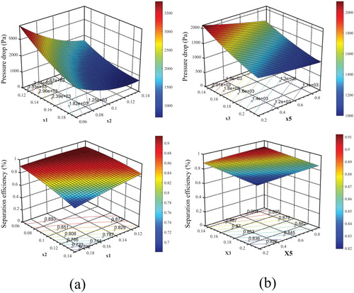
Table 7. Results for fitting of regression coefficient of RSM η model and ANOVA results for RSM term.

Terms	Regression coefficient of RSM (η)	F-Value	P-Value
${\text{β}}_0$	0.052	91.86	0
Linear		293.32	0
${\text{β}}_1$	5.41	269.26	0
${\text{β}}_2$	8.16	724.9	0
${\text{β}}_3$	3.24	139.74	0
${\text{β}}_4$	−0.21	39.4	0
Quadratic		5.09	0.017
${\text{β}}_1$^2	−5.76	1.46	0.255
${\text{β}}_2$^2	−15.13	10.08	0.01
${\text{β}}_3$^2	1.12	0.06	0.819
${\text{β}}_4$^2	−0.0262	0.18	0.683
Interaction		15.41	0
${\text{β}}_1$*${\text{β}}_2$	−25.47	40.46	0
${\text{β}}_1$*${\text{β}}_3$	−17.03	18.09	0.002
${\text{β}}_1$*${\text{β}}_4$	1.411	9.5	0.012
${\text{β}}_2$*${\text{β}}_3$	−19.22	23.04	0.001
${\text{β}}_2$*${\text{β}}_4$	0.518	1.28	0.284
${\text{β}}_3$*${\text{β}}_4$	0.125	0.07	0.79

$\begin{array}{l}{y}_1=0.052+5.41{\text{x}}_1+8.16{\text{x}}_2+3.24{\text{x}}_3-0.210{\text{x}}_5-5.76{\text{x}}_1^2-15.13{\text{x}}_2^2\\ +1.12{\text{x}}_3^2-0.0262{\text{x}}_5^2-25.47{\text{x}}_1{\text{x}}_2-17.03{\text{x}}_1{\text{x}}_3+1.411{\text{x}}_1{\text{x}}_5\\ -19.22{\text{x}}_2{\text{x}}_3+0.518{\text{x}}_2{\text{x}}_5+0.125{\text{x}}_3{\text{x}}_5\end{array}$

Table 8. Results for fitting of regression coefficient of RSM Δp model and ANOVA results for RSM term.

Terms	Regression coefficient of RSM $\mathrm{\Delta }$p	F-Value	P-Value
${\text{β}}_0$	23764	417.83	0
Linear		1404.43	0
${\text{β}}_1$	−98913	2296.44	0
${\text{β}}_2$	−118886	2636.12	0
${\text{β}}_3$	−52739	535.58	0
${\text{β}}_4$	−3726	149.58	0
Quadratic		27.99	0
${\text{β}}_1$^2	147586	26.7	0
${\text{β}}_2$^2	217493	57.98	0
${\text{β}}_3$^2	42547	2.22	0.167
${\text{β}}_4$^2	162	0.19	0.673
Interaction		20	0
${\text{β}}_1$*${\text{β}}_2$	168230	49.14	0
${\text{β}}_1$*${\text{β}}_3$	81943	11.66	0.007
${\text{β}}_1$*${\text{β}}_4$	8536	9.69	0.011
${\text{β}}_2$*${\text{β}}_3$	141231	34.64	0
${\text{β}}_2$*${\text{β}}_4$	9668	12.43	0.005
${\text{β}}_3$*${\text{β}}_4$	4298	2.46	0.148

$\begin{array}{l}{\text{y}}_2=23764-98913{\text{x}}_1-118886{\text{x}}_2-52739{\text{x}}_3-3726{\text{x}}_5+147586{\text{x}}_1^2\\ +217493{\text{x}}_2^2+42547{\text{x}}_3^2+162{\text{x}}_5^2+168230{\text{x}}_1{\text{x}}_2+81943{\text{x}}_1{\text{x}}_3\\ +8536{\text{x}}_1{\text{x}}_5+141231{\text{x}}_2{\text{x}}_3+9668{\text{x}}_2{\text{x}}_5+4298{\text{x}}_3{\text{x}}_5\end{array}$

The ANOVA showed that the coefficient of determination (R²) of the $\mathrm{\Delta }\text{p}$ and the η are 99.83% and 99.21% using CCD results (train set), respectively. The adjusted coefficient of determination (${\text{R}}_{\text{adj}}^2$) of the $\mathrm{\Delta }\text{p}$ and the η considering the degree of freedom of the variables were 99.62% and 98.29% about train set, respectively. However, the RSM model should be evaluated for accurate prediction performance by using a test set that is not used for model parameter estimation rather than train set.

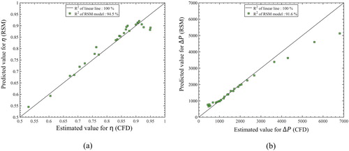
Therefore, the predictive performance of the RSM cyclone models was evaluated based on the CFD test set as shown Figure 9. The R² values of the $\mathrm{\Delta }\text{p}$ and η were 91.61% and 94.5%, respectively. In particular, the RSM model has relatively poor predictive performance for collection efficiency data> 92% and pressure drop data> 4000 Pa. Consequently, this indicates that the RSM cyclone models have relatively low predictability for the new data.

Figure 9. Prediction performance results of cyclone RSM model for (a) separation efficiency and (b) pressure drop.

3.6.2. Modeling for η and $\mathrm{\Delta }\text{p}$ using GMDH-type neural network

The coefficient of GMDH polynomial for η and $\mathrm{\Delta }\text{p}$ is obtained as Tables 9 and 10, respectively. The adequacy of GMDH model for η and $\mathrm{\Delta }\text{p}$ was evaluated by analyzing agreement between the cyclone GMDH output and the CFD test sets output. Figure 10 (a, b) present comparison of the prediction results of the performance parameters using GMDH with CFD results including x-y line. The predictive performance of the obtained the GMDH cyclone models were evaluated quantitatively based on the correlation coefficient. The correlation coefficients of η and Δp were 98.9%, 99.7%, respectively. The predictive performance of the obtained the GMDH cyclone models were evaluated quantitatively using the correlation coefficient. As shown Figure 10, the GMDH cyclone models predicted effectively the estimated values by CFD.

Figure 10. Prediction performance results of GMDH cyclone model for (a) separation efficiency and (b) pressure drop.

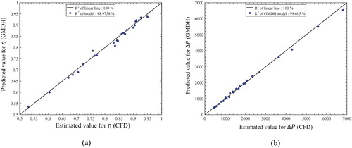
Table 9. GMDH η model.

Layer number	GMDH model for η
(1)
	$\begin{array}{l}Y{1^{\mathrm{\prime }}}_{\left(1\right)}=0.877+0.107D_{\mathrm{X}}+2.6872a+1.031D_{\mathrm{X}}^2\text{--}12.18a^2-14.17D_{\mathrm{X}}\ast a\\ Y{2^{\mathrm{\prime }}}_{\left(1\right)}=0.784+1.751\text{a}+1.658\text{b}-9.74\text{a}2\text{--}4.23\text{b}2-9.73\text{a}\ast \text{b}\\ Y{3^{\mathrm{\prime }}}_{\left(1\right)}=0.902+0.259a+0.069H_{\text{co}}-10.75a^2-0.035H_{\text{co}}^2+0.115\text{a}\ast H_{\text{co}}\\ Y{4^{\mathrm{\prime }}}_{\left(1\right)}=0.085+1.521D_{\mathrm{X}}+0.199b-5.09D_{\mathrm{X}}^2-0.247b^2\text{--}5.44D_{\mathrm{X}}\ast b\end{array}$
(2)
	$\begin{array}{l}Y{1^{\mathrm{\prime }}}_{\left(2\right)}=-10+13.02Y{3^{\mathrm{\prime }}}_{\left(1\right)}+11.39Y{4^{\mathrm{\prime }}}_{\left(1\right)}-1.332Y{3}_{\left(1\right)}^{\mathrm{\prime }2}-0.325Y{4}_{\left(1\right)}^{\mathrm{\prime }2}-11.4Y{3^{\mathrm{\prime }}}_{\left(1\right)}\ast Y{4^{\mathrm{\prime }}}_{\left(1\right)}\\ Y{2^{\mathrm{\prime }}}_{\left(2\right)}=-1.11+3.97Y{2^{\mathrm{\prime }}}_{\left(1\right)}-1.21Y{4^{\mathrm{\prime }}}_{\left(1\right)}+1.64Y{2}_{\left(1\right)}^{\mathrm{\prime }2}+4.61Y{4}_{\left(1\right)}^{\mathrm{\prime }2}-6.81Y{2^{\mathrm{\prime }}}_{\left(1\right)}\ast Y{4^{\mathrm{\prime }}}_{\left(1\right)}\\ Y{3^{\mathrm{\prime }}}_{\left(2\right)}=-3.65+3.63Y{1^{\mathrm{\prime }}}_{\left(1\right)}+5.57Y{4^{\mathrm{\prime }}}_{\left(1\right)}+1.28Y{1}_{\left(1\right)}^{\mathrm{\prime }2}-0.135Y{4}_{\left(1\right)}^{\mathrm{\prime }2}-5.73Y{1^{\mathrm{\prime }}}_{\left(1\right)}\ast Y{4^{\mathrm{\prime }}}_{\left(1\right)}\\ Y{4^{\mathrm{\prime }}}_{\left(2\right)}=-1.73+2.46Y{1^{\mathrm{\prime }}}_{\left(1\right)}+2.53Y{2^{\mathrm{\prime }}}_{\left(1\right)}+1.764Y{1}_{\left(1\right)}^{\mathrm{\prime }2}+1.603Y{2}_{\left(1\right)}^{\mathrm{\prime }2}-5.65Y{1^{\mathrm{\prime }}}_{\left(1\right)}\ast Y2\end{array}$
(3)	$Y_{\left({\eta }_{-}\text{output}\right)}=0.243+1.434Y{1}_{\left(2\right)}^{\mathrm{\prime }}-1.01Y{2}_{\left(2\right)}^{\mathrm{\prime }}-3.399Y{1}_{\left(2\right)}^{\mathrm{\prime }2}-2.404Y{2}_{\left(2\right)}^{\mathrm{\prime }2}+6.14Y{1}_{\left(2\right)}^{\mathrm{\prime }}\ast Y{2}_{\left(2\right)}^{\mathrm{\prime }}$

Table 10. GMDH $\mathrm{\Delta }$p model.

Layer number	GMDH model for $\mathrm{\Delta }$p
(1)
	$\begin{array}{l}Y{1}_{\left(1\right)}=15366-90840D_X-85572a-178194D_{\mathrm{X}}^2\text{--}182057a^2+169080D_{\mathrm{X}}\ast a\\ Y{2}_{\left(1\right)}=7020-66939a-1266b+215008a^2\text{--}20596b^2+4221a\ast b\\ Y{3}_{\left(1\right)}=6587\text{--}65887a\text{--}1373H_{\text{co}}+2118802a^2+508H_{\text{co}}^2+2420a\ast H_{\text{co}}\\ Y{4}_{\left(1\right)}=9641\text{--}46907D_{\mathrm{X}}-24054b+100521D_{\mathrm{X}}^2+56256b^2\text{--}22432D_{\mathrm{X}}\ast b\end{array}$
(2)
	$\begin{array}{l}Y{1}_{\left(2\right)}=579-0.178Y{3}_{\left(1\right)}-0.739Y{4}_{\left(1\right)}+0.00075Y{3}_{\left(1\right)}^2+0.00022Y{4}_{\left(1\right)}^2+0.00049Y{3}_{\left(1\right)}\ast Y{4}_{\left(1\right)}\\ Y{2}_{\left(2\right)}=313-0.12Y{2}_{\left(1\right)}-0.28Y{4}_{\left(1\right)}+0.00061Y{2}_{\left(1\right)}^2+0.0001Y{4}_{\left(1\right)}^2+0.00045Y{2}_{\left(1\right)}\ast Y{4}_{\left(1\right)}\\ Y{3}_{\left(2\right)}=90+0.75Y{1}_{\left(1\right)}+0.01Y{2}_{\left(1\right)}-0.00082Y{1}_{\left(1\right)}^2-0.00053Y{2}_{\left(1\right)}^2+0.00023Y{1}_{\left(1\right)}\ast Y{2}_{\left(1\right)}\\ Y{4}_{\left(2\right)}=-234+0.737Y{1}_{\left(1\right)}+0.39Y{4}_{\left(1\right)}-0.00011Y{1}_{\left(1\right)}^2-0.00018Y{4}_{\left(1\right)}^2+0.00031Y{1}_{\left(1\right)}\ast Y{4}_{\left(1\right)}\end{array}$
(3)
	$\begin{array}{l}Y{1}_{\left(3\right)}=-149+0.59Y{1}_{\left(2\right)}+0.61Y{4}_{\left(2\right)}+0.00026Y{1}_{\left(2\right)}^2-0.00011Y{4}_{\left(2\right)}^2-0.00021Y{1}_{\left(2\right)}\ast Y{4}_{\left(2\right)}\\ Y{2}_{\left(3\right)}=-155.7+0.55Y{1}_{\left(2\right)}+0.65Y{3}_{\left(2\right)}+0.00011Y{1}_{\left(2\right)}^2-0.00026Y{3}_{\left(2\right)}^2+0.00091Y{1}_{\left(2\right)}\ast Y{3}_{\left(2\right)}\\ Y{3}_{\left(3\right)}=-3.249+0.7478Y{1}_{\left(2\right)}+0.2454Y{2}_{\left(2\right)}-0.00014Y{1}_{\left(2\right)}^2-0.00017Y{2}_{\left(2\right)}^2+0.00033Y{1}_{\left(2\right)}\ast Y{2}_{\left(2\right)}\\ Y{4}_{\left(3\right)}=-107.88+0.655Y{2}_{\left(2\right)}+0.4296Y{4}_{\left(2\right)}-0.00016Y{2}_{\left(2\right)}^2-0.00017Y{4}_{\left(2\right)}^2+0.00033Y{2}_{\left(2\right)}\ast Y{4}_{\left(2\right)}\end{array}$
(4)	$Y_{(\mathrm{\Delta }}p{}_{-}\mathrm{o}\mathrm{u}\mathrm{t}\mathrm{p}\mathrm{u}\mathrm{t})=3.304+0.652Y{1}_{\left(3\right)}+0.335Y{4}_{\left(3\right)}-0.00013Y{1}_{\left(3\right)}^2-0.00021Y{4}_{\left(3\right)}^2+0.00035Y{1}_{\left(3\right)}\ast Y{4}_{\left(3\right)}$

3.6.3. Modeling for η and $\mathrm{\Delta }\text{p}$ using BPNN

The prediction performance of the ANN model depends on the number of neurons and the number of layers. If the number of datasets is small, larger the number of layers, and larger the overfitting that causes problem in prediction performance of new dataset (Onwubolu, 2015).

So, in this study, the best network architecture has been investigated by grid search method (trial and error method). Based on the grid search method, the root mean square error (RMSE) of each BPNN model for the cyclone performance parameters was measured according to increasing the number of nodes and number of layers as shown Figure 11. As shown in the Fig. 11(a), RMSE of $\eta$ model is overfitted when the number of nodes is more than 14 and the number of layers is more 3.

Figure 11. Results of hyperparameter tuning (a) separation efficiency and (b) pressure drop; from up to down: number of node and number of layer.

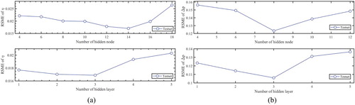
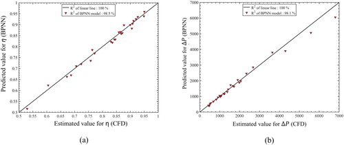
Also, Figure 11(b) presents that the RMSE of the $\mathrm{\Delta }\text{p}$ model is overfitted when the number of nodes is more than 8 nodes and the number of layers is more 3. Therefore, the RMSE of the BPNN model of $\mathrm{\Delta }\text{p}$ and $\eta$ with optimal structure was 0.12 and 0.16, respectively. Figure 12 present the prediction performance for BPNN cyclone model based on the CFD test set. It showed the result of the prediction performance in the optimal BPNN structure, which is a good agreement, and the R² for $\mathrm{\Delta }\text{p}$ and $\eta$ was 98.1 and 98.5, respectively.

Figure 12. Prediction performance results of BPNN cyclone model for (a) separation efficiency and (b) pressure drop.

3.6.4. Comparison of prediction performance among RSM, GMDH and BPNN for $\mathrm{\Delta }\text{p}$ and $\text{η}$

In this study, the predictive model for Δp and η were obtained using RSM, GMDH and BPNN algorithm. In order to compare the prediction accuracy for the predictive models, the histogram of the error distributions and the prediction behavior for the three η models and three Δp models were analyzed using the CFD test set as shown Figures 13 and 14, respectively. The histogram of the error distributions can give better comparison for the prediction performance in terms of the possible error ranges (Onwubolu, 2015). The frequency of error between the prediction results by the developed cyclone models and the estimated results by CFD was normalized for convenient.

Figure 13. Comparison analysis of prediction performance test of separation efficiency model using RSM, GMDH and BPNN based the CFD test set; (a) Error histogram and probability density function for difference between CFD result and prediction value by models (b) Error value between CFD result and prediction value by models.

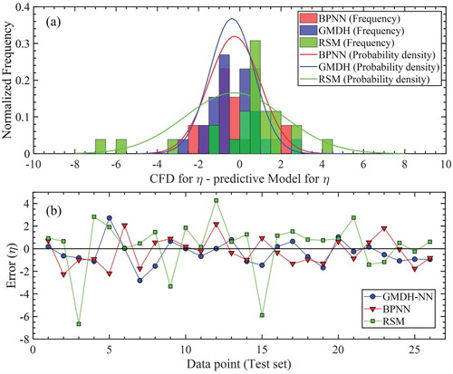
Figure 14. Comparison analysis of prediction performance test of pressure drop model using RSM, GMDH and BPNN based the CFD test set; (a) Error histogram and probability density function for difference between CFD result and prediction value by models (b) Error value between CFD result and prediction value by models

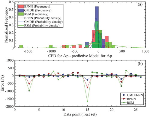
As shown Figures. 13 and 14, the probability density function and the frequency the error were widely distributed in RSM cyclone model for η and $\mathrm{\Delta }\text{p}$, compared to the neural network approaches. It showed low predictive performance of the RSM cyclone model. On the other hand, the GMDH results and BPNN results have higher prediction accuracy because the neural network approaches are considered for high-order nonlinearities unlike RSM approaches. Also, the predictive performance of RSM is especially poor at data points (3, 10, 22) for collection efficiency and pressure drop. In case of the data points, the flow rate is the same, but the inlet area is reduced, and the exit diameter of the cyclone is reduced, which increases the inlet velocity, resulting in a strong vortex with a physically sharp pressure gradient inside the cyclone. The GMDH and BPNN models with higher terms than the RSM show relatively good results in order to predict this sudden increase in pressure gradient. When comparing the BPNN results and the GMDH results, the variance of the error histogram of the BPNN model and the GMDH model was quite similar. However, training in the GMDH is based on performing linear algebra which requires short time for convergence rather than an iterative method of minimizing the error like the back-propagation algorithm which requires a large amount of time for convergence (Hagan et al., 1997). The convergence speed of the GMDH model of $\mathrm{\Delta }\text{p}$ and $\eta$ (41 sec) was 15 times lower than that of BPNN model (621 sec).

Moreover, the GMDH cyclone models are mathematically expressed as a higher-order polynomial model. However, in the case of the BPNN cyclone model, the obtained model is still hidden as the black box model. The neural structure (the number of layer) for the BPNN cyclone models were 4. The neural structure for GMDH's $\mathrm{\Delta }\text{p}$, $\eta$ model were 4, 3, respectively. The BPNN algorithm needs to select the optimum neural structure by adjusting the hyperparameter, while the GMDH algorithm can adaptively optimize the structure to avoid overfitting problem.

Errors between predicted values by each model and estimated values at each CFD test set are shown in Figures 13 (b) and 14(b). It shown that the error of GMDH models is close to zero at all data point, compared to RSM and BPNN. Also, Table 11 presents the predictive performance of the three models using R², RMSE, ${\text{R}}_{\text{adjusted}}^2$ and AIC based on the CFD test sets. The AIC and ${\text{R}}_{\text{adjusted}}^2$ evaluate the overfit risk and underfit risk of the model. As shown Table 11, the GMDH cyclone models (Δp: $R^2=99.7$, RMSE = 0.102, $R_{\text{adjusted}}^2=98.4$, AIC = 36.794 and η: $R^2=98.99$, RMSE = 0.0119, $R_{\text{adjusted}}^2=94.45$, AIC = 186.64) showed the best prediction performance than other models.

Table 11. Predictive model comparison of η and Δp parameters obtained by RSM, GMDH and BPNN.

	RSM		GMDH		ANN
	η	$\mathrm{\Delta }$p	η	$\mathrm{\Delta }$p	η	$\mathrm{\Delta }$p
R^2 (%)	94.5	91.6	98.98	99.69	98.5	98.1
RMSE	0.023	0.235	0.012	0.103	0.017	0.106
${\text{R}}_{\text{adjusted}}^2$	93.5	90.22	97.88	99.3	97.44	96.38
AIC	225.24	118.92	186.64	36.8	220.13	72.53

Furthermore, in order to quantitatively estimate and compare the uncertainties of the cyclone models, uncertainty analysis (Gholami et al., 2018) was performed with the 25 CFD test set. To estimate the uncertainties, prediction error (PE), mean prediction error (MPE), standard deviation of prediction error (SDPE) and width of uncertainty band (WUB) and prediction error interval of 95% (PEI) are introduced. The value of MPE indicates an overestimated model for positive numbers and an underestimated model for negative numbers. The WUB and PEI can be expressed by the SDPE. (28) $\begin{array}{rl}\text{MPE}& =\sum _{i=1}^n{e}_j=\sum _{i=1}^n(P_i-T_i)\end{array}$(28) (29) $\begin{array}{rl}\text{SDPE}& =\sqrt{\frac{\sum _{i=1}^n\left(e_j-\text{MPE}\right)}{n-1}}\end{array}$(29) (30) $\begin{array}{rl}\text{PEI}& =\pm 1.96\ast \text{SDPE}\end{array}$(30)

Where, $P_i$ is the predicted value, $T_i$ is the estimated value. The uncertainty analysis results for the all cyclone models are shown in Table 12. The WUB of GMDH models showed the lowest values ($\eta$ = ±0.0065, Δp = ±0.0188) compared to the RSM and the BPNN results. Also, it was seen that the model of smallest MPE and 95% PEI are the GMDH model. Furthermore, the width of uncertainty band between the estimated values by CFD and the predicted values by the three models were visualized in Figure 15. The upper line and lower line of 95% PEI for $\eta$ and Δp predicted by GMDH are best distributed in the exact line. Therefore, the GMDH cyclone models for Δp and $\eta$ was reasonably selected as the optimal predictive model in this paper. The GMDH cyclone models for Δp and $\eta$ are used in next section for the Pareto multi-objective optimization.

4. Multi-objective optimization for $\text{η}$ and $\mathbf{\Delta }\mathbf{\text{p}}$ by using genetic algorithm

4.1. Genetic algorithm

GA (Genetic Algorithms) are one of the optimization methods to solve local optimization problem. The GA inspired by the natural evolution. The population evolves towards the optimal form under the natural conditions. The GA repeatedly updates the population of individual solutions. In each step of the GA process, the GA produces initial random population and evaluates fitness for the individual. The best individuals are selected as the parent, and then the GA produces the offspring by applying crossover and mutation for the next generation. The GA is terminated when it reaches to the certain criterion.

Figure 15. Comparison analysis of qualitative scatter plot about width of uncertainty band of (a) Separation efficiency model and (b) Pressure drop model by three proposed method (BPNN, GMDH and RSM).

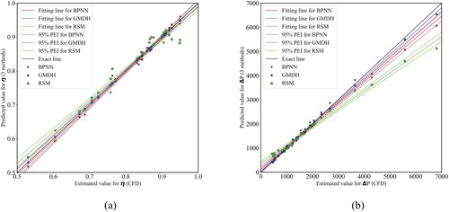
Table 12. Uncertainty analysis results for cyclone performance models of GMDH, BPNN and RSM.

Models	# Number of samples	MPE	SDPE	WUB	95% PEI
GMDH for η	25	0.023	0.0218	±0.0065	(0.016 0.029)
BPNN for η	25	0.029	0.0288	±0.0085	(0.021 0.037)
RSM for η	25	0.039	0.0478	±0.0132	(0.025 0.523)
GMDH for Δp	25	0.019	0.0865	±0.0188	(0.002 0.038)
BPNN for Δp	25	0.057	0.208	±0.0464	(0.011 0.103)
RSM for Δp	25	0.1105	0.416	±0.0955	(0.015 0.206)

However, in the many multi-optimization problems, the objective functions conflicted with each other. Therefore, it is hard to obtain the best optimized points to optimize all objective functions simultaneously. For solving the problem, Den, Agrawal, Pratap, and Meyarivan (2000) proposed the non-dominant genetic algorithm-II (NSGA-II). The non-dominated solutions set (also expressed as Pareto optimal front) provide the optimal solution by determining the point among solution set. For more details about the GA, see the Ref (Elsayed & Lacor, 2013).

4.2. Results of multi-objective optimization for Δp and $\text{η}$ using NSGA-II

For multi-objective optimization for Δp and $\eta$, the non-dominated solutions set was obtained by NSGA-II using MATLAB 2018a. Table 13 presents a setting condition for multi-objective optimization. The conditions in NSGA-II were set up to search the entire design area. The fitness functions from GMDH-cyclone model for Δp and η were used for the GA optimization. The constraints of geometrical parameters used in the GA optimization are same as range of parameters at Table 3.

Table 13. Genetic algorithm setup for multi-objective optimization.

Population type	Double vector
Fitness scaling	Rank
Selection operation	Roulette method
Crowding distance fraction	0.35
Crossover fraction	0.8
Crossover operation	Intermediate crossover with the default value of 1.0
Mutation operation	The constraint dependent default
Maximum number of generations	1000
Population size	120

Figure 16 presents the results of 70 Pareto optimal front for η and Δp. The η is expressed as negative for the optimization purpose. The five design points (A,B,C,D,E) from 70 Pareto optimal front were determined to decide the optimal Δp and η. Point A have the high pressure drop compared to other point, it may require the high power to operate the manufacturing system. Point E has the low collection efficiency compared to other point. It cannot function properly as a cyclone. Point C was chosen to optimization cycle. The separation efficiency and pressure drop of Point C are 91.1% and 98.5 Pa, respectively, it has good performance compared the reference data. Also, Table 14 shows the reproducibility results. The reproducibility results show that GMDH cyclone models have high predictive performance.

Figure 16. Pareto front for multi-objective optimization for cyclone performance parameters.

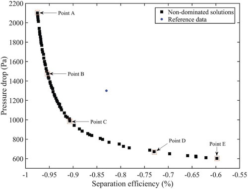
Table 14. Validation of Pareto optimal front for the cyclone performance.

					GA results		CFD results		Error (%)
	$D_x$ (x1)	$a$ (x2)	b (x3)	$H_{co}$ (x4)	η (%)	Δp (Pa)	η (%)	Δp (Pa)	η	Δp
Point A	0.059	0.135	0.185	0.9	0.97	2072	0.93	2144	4.3	3.35
Point B	0.085	0.135	0.185	0.9	0.93	1351	0.91	1349	2.15	0.15
Point C	0.105	0.1385	0.187	0.87	0.91	984	0.88	970	3.29	1.42
Point D	0.116	0.175	0.189	0.8	0.79	725	0.78	689	1.26	4.96
Point E	0.126	0.213	0.192	0.24	0.61	618	0.58	563	4.91	8.89

Finally, Table 15 shows the improvement rate of Δp and η of the optimized cyclone and the dimension ratio of the optimized cyclone. The η, d50 and Δp of optimized cyclones improved 8.79%, 18%, and 24.31% respectively over the performance of the reference cyclone. Figure 17 presents the comparison of the collection efficiency curve between the reference cyclone and the optimization cyclone. It presented that the collection efficiency for particles less than 1 micron was improved by about 20%. Figure 18 presents the particle behavior in the optimized cyclone. Therefore, the optimized cyclone demonstrates a reasonable approach in the GMDH-type neural network combined DOE and NSGA-II optimization processes in the present work.

Figure 17. Comparison of the separation efficiency curve between the optimized cyclone and the reference model.

note: unit % is multiplied by 100.

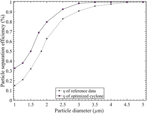
Figure 18. The behavior when the particles of different sizes (1–10 $\mu m$)are injected into the optimized cyclone.

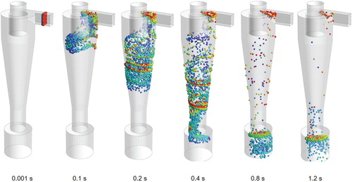
Table 15. Comparison of results for cyclone performance parameters between optimized cyclones and reference model.

	$D_x$ (x1)	$a$ (x2)	b (x3)	$H_{co}$ (x4)	η (%)	Δp (Pa)	Cut-off size ($\text{μ}\text{m}$)
Reference model	0.15	0.1	0.175	0.49	0.83	1300	1.83
Optimized model	0.105	0.1385	0.187	0.87	0.91	984	1.5
Improvement (%)	30	−38.5	−6.85	−77.55	8.79	24.31	18.03

4.3. Results of numerical simulation comparison between optimized cyclone and reference model

In order to analyze why the optimized cyclone model could achieve better performance than the reference model, the flow pattern of optimized cyclone was compared with the reference model by using CFD. The secondary circulation in cyclone decreases the cyclone separation performance due to particle re-entrainment phenomenon. Figure 19(a) presents the comparison for velocity vector field of the optimized cyclone and reference cyclone. The secondary circulation occurred at the reference cyclone. However, the optimized cyclone showed that the area of secondary circulation was decreased as shown Figure 19(a), compared to reference model. Therefore, when compared with reference cyclone, the separation efficiency of optimization cyclone outperform.

Figure 19. Results of flow pattern analysis; from left to right: Reference cyclone and optimized cyclone; (a) comparison for velocity vector field. (b) comparison for pressure drop. (c) comparison for turbulent kinetic energy.

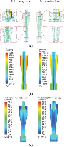
The contour of pressure drops of the optimized cyclone and reference cyclone presents in Figure 19(b), respectively. The maximum pressure of the optimized cyclone was about 200 lowers than the reference cyclone. This high pressure drop requires the high power to operate the manufacturing system and affects exposure of the particles in the cyclone called the phenomenon of ‘lip leakage’. This resulted in an improvement in the cyclone separation performance.

Figure 19(c) presents the turbulent kinetic energy (TKE) of the reference cyclone and the optimized cyclone. As shown in the Figure 19(e), the TKE was observed relatively high near the cyclone vortex finder of the reference model. As the TKE increases, the collection efficiency decreases. The maximum TKE of the optimized cyclone decreased by 25%, compared to the reference cyclone.

5. Conclusion

This study performed a comparative study among RSM, BPNN and GMDH algorithm for predictive models of Δp and $\eta$, and multi-objective cyclone optimization was successfully performed by using NSGA-II. In this study, MM model was selected as the reference model, and the optimization objectives were defined to minimize Δp and maximize η. After the DOE analysis for the cyclone geometric parameters using the validated CFD, the predictive models for Δp and η were obtained based on RSM, GMDH technique and BPNN technique. As a result of comparing the obtained models, the GMDH cyclone models predicted the Δp and η most efficiently. The R² of η and Δp was 98.9%, 99.7%, respectively. Therefore, the GMDH cyclone models were used in the GA as the fitness functions. A total of 70 non-dominated optimal design points were obtained by GA. The five optimal point were selected to validate accuracy of GA results using CFD. The reproducibility results showed less than 10% error and proved the reliability of the GA optimization process. The optimized cyclone (Point C) provided a more reasonable improvement than the MM model. The optimized cyclone reduced the pressure drop by 24.31% (from 1300 to 984 Pa), the cut-off diameter by 18% (from 1.83 μm to 1.5 μm) and increased the overall efficiency by 8.79% (from 83% to 91%). In addition, the optimized reason was demonstrated by analysis of the flow part of the cyclone (flow field, pressure drop, turbulence kinetic energy).

The results presented can help with selection of appropriate prediction modeling techniques about the cyclone, and the obtained 70 Pareto front design points can assist designers and decision makers to optimize cyclone design. However, the optimization results need to be verified using experimental methods in addition to CFD. Therefore, future studies will further demonstrate the feasibility of the research by fabricating the cyclone based on optimized cyclone dimensions and conducting experiments on separation performance and pressure drop.

Disclosure statement

No potential conflict of interest was reported by the authors.

References

- ANSYS FLUENT, 16.1. (2016). User’s and theory guide. Canonsburg, PA, USA: ANSYS, Inc.
- Ardabili, S. F., Najafi, B., Shamshirband, S., Bidgoli, B. M., Deo, R. C., & Chau, K. W. (2018). Computational intelligence approach for modeling hydrogen production: A review. Engineering Applications of Computational Fluid Mechanics, 12, 438–458. doi:10.1080/19942060.2018.1452296
- Avci, A., & Karagoz, I. (2001). Theoretical investigation of pressure losses in cyclone separators. International Communications in Heat and Mass Transfer, 28, 107–117. doi:10.1016/S0735-1933(01)00218-4
- Barth, W. (1956). Design and layout of the cyclone separator on the basis of new investigations. Brennstow-Wäerme-Kraft (BWK), 8(4), 1–9.
- Bernardo, S., Mori, M., Peres, A. P., & Dionísio, R. P. (2006). 3-D computational fluid dynamics for gas and gas-particle flows in a cyclone with different inlet section angles. Powder Technology, 162, 190–200. doi:10.1016/j.powtec.2005.11.007
- Boyan, F., Ayers, W. H., & Swithenbank, J. (1982). A Fundamental mathematical modeling approach to cyclone design. Transactions of the Institution of Chemical Engineers, 60, 222–230.
- Brar, L. S., Sharma, R. P., & Elsayed, K. (2015). The effect of the cyclone length on the performance of Stairmand high-efficiency cyclone. Powder Technology, 286, 668–677. doi:10.1016/j.powtec.2015.09.003
- Den, K., Agrawal, S., Pratap, A., & Meyarivan, T. (2000). A fast elitist non-dominated sorting genetic algorithm for multi-objective optimization: NSGA-II. International Conference on Parallel Problem Solving from Nature, 849–858. doi:10.1007/3-540-45356-3_83
- De Souza, F. J., Salvo, R. D. V., & Martins, D. D. M. (2015). Effects of the gas outlet duct length and shape on the performance of cyclone separators. Separation and Purification Technology, 142, 90–100. doi:10.1016/j.seppur.2014.12.008
- Dietz, P. W. (1981). Collection efficiency of cyclone separators. AIChE Journal, 27, 888–892. doi:10.1002/aic.690270603
- Ebtehaj, I., & Bonakdari, H. (2016). Assessment of evolutionary algorithms in predicting non-deposition sediment transport. Urban Water Journal, 13, 499–510. doi:10.1080/1573062X.2014.994003
- Elsayed, K., & Lacor, C. (2011). The effect of cyclone inlet dimensions on the flow pattern and performance. Applied Mathematical Modelling, 35, 1952–1968. doi:10.1016/j.apm.2010.11.007
- Elsayed, K., & Lacor, C. (2012). Modeling and Pareto optimization of gas cyclone separator performance using RBF type artificial neural networks and genetic algorithms. Powder Technology, 217, 84–99. doi:10.1016/j.powtec.2011.10.015
- Elsayed, K., & Lacor, C. (2013). CFD modeling and multi-objective optimization of cyclone geometry using desirability function, artificial neural networks and genetic algorithms. Applied Mathematical Modelling, 37, 5680–5704. doi:10.1016/j.apm.2012.11.010
- Fotovatikhah, F., Herrera, M., Shamshirband, S., Chau, K. W., Ardabili, S. F., & Piran, M. J. (2018). Survey of computational intelligence as basis to big flood management: Challenges, research directions and future work. Engineering Applications of Computational Fluid Mechanics, 12, 411–437. doi:10.1080/19942060.2018.1448896
- Ganegama Bogodage, S., & Leung, A. Y. T. (2015). CFD simulation of cyclone separators to reduce air pollution. Powder Technology, 286, 488–506. doi:10.1016/j.powtec.2015.08.023
- Gholami, A., Bonakdari, H., Ebtehaj, I., Mohammadian, M., Gharabaghi, B., & Khodashenas, S. R. (2018). Uncertainty analysis of intelligent model of hybrid genetic algorithm and particle swarm optimization with ANFIS to predict threshold bank profile shape based on digital laser approach sensing. Measurement: Journal of the International Measurement Confederation, 121, 294–303. doi:10.1016/j.measurement.2018.02.070
- Gimbun, J., Chuah, T. G., Choong, T. S. Y., & Fakhru’l-Razi, A. (2005). A CFD study on the prediction of cyclone collection efficiency. International Journal of Computational Methods in Engineering Science and Mechanics, 6, 161–168. doi:10.1080/15502280590923649
- Hagan, M. T., Demuth, H. B., & Beale, M. (1997).Neural network design. Boston: PWS Publishing Co.
- Hamdy, O., Bassily, M. A., El-Batsh, H. M., & Mekhail, T. A. (2017). Numerical study of the effect of changing the cyclone cone length on the gas flow field. Applied Mathematical Modelling, 46, 81–97. doi:10.1016/j.apm.2017.01.069
- Hoffmann, A. C., & Stein, L. E. (2008).Gas cyclones and Swirl Tubes: Principle, design and operation (2nd ed.). Berlin: Springer.
- Kaya, F., & Karagoz, I. (2009). Numerical investigation of performance characteristics of a cyclone prolonged with a dip leg. Chemical Engineering Journal, 151, 39–45. doi:10.1016/j.cej.2009.01.040
- Khalkhali, A., & Safikhani, H. (2012). Pareto based multi-objective optimization of a cyclone vortex finder using CFD, GMDH type neural networks and genetic algorithms. Engineering Optimization, 44, 105–118. doi:10.1080/0305215X.2011.564619
- Khayet, M., Cojocaru, C., & Essalhi, M. (2011). Artificial neural network modeling and response surface methodology of desalination by reverse osmosis. Journal of Membrane Science, 368, 202–214. doi:10.1016/j.memsci.2010.11.030
- Leith, D. (1990). The logistic function and cyclone fractional efficiency. Aerosol Science and Technology, 12, 598–606. doi:10.1080/02786829008959373
- Mathews, P. (2005). Design of experiments with MINITAB. Milwaukee: ASQ Quality Press.
- Moazenzadeh, R., Mohammadi, B., Shamshirband, S., & Chau, K. W. (2018). Coupling a firefly algorithm with support vector regression to predict evaporation in northern Iran. Engineering Applications of Computational Fluid Mechanics, 12, 584–597. doi:10.1080/19942060.2018.1482476
- Muschelknautz, E., & Krambrock, W. (1970). AerodynamischeBeiwerte des Zyklonabscheidersaufgrundneuer und verbesserterMessungen. Chemie Ingenieur Technik - CIT, 42, 247–255. doi:10.1002/cite.330420503
- Najafi, B., Faizollahzadeh Ardabili, S., Shamshirband, S., Chau, K. W., & Rabczuk, T. (2018). Application of anns, anfis and rsm to estimating and optimizing the parameters that affect the yield and cost of biodiesel production. Engineering Applications of Computational Fluid Mechanics, 12, 611–624. doi:10.1080/19942060.2018.1502688
- Obermair, S., & Staudinger, G. (2001). The dust outlet of a gas cyclone and its effects on collection efficiency. Chemical Engineering & Technology, 24, 1259–1263. doi:10.1002/1521-4125(200112)24:12<1259::AID-CEAT1259>3.0.CO;2-O
- Obermair, S., Woisetschläger, J., & Staudinger, G. (2003). Investigation of the flow pattern in different dust outlet geometries of a gas cyclone by laser Doppler anemometry. Powder Technology, 138, 239–251. doi:10.1016/j.powtec.2003.09.009
- Onwubolu, G. (2015). GMDH methodology and implementation in MATLAB. London: Imperial College Press.
- Qian, F., Zhang, J., & Zhang, M. (2006). Effects of the prolonged vertical tube on the separation performance of a cyclone. Journal of Hazardous Materials, 136, 822–829. doi:10.1016/j.jhazmat.2006.01.028
- Rahimpour, F., Hatti-Kaul, R., & Mamo, G. (2016). Response surface methodology and artificial neural network modelling of an aqueous two-phase system for purification of a recombinant alkaline active xylanase. process Biochemistry, 51, 452–462. doi:10.1016/j.procbio.2015.12.018
- Raoufi, A., Shams, M., Farzaneh, M., & Ebrahimi, R. (2008). Numerical simulation and optimization of fluid flow in cyclone vortex finder. Chemical Engineering and Processing: Process Intensification, 47, 128–137. doi:10.1016/j.cep.2007.08.004
- Safikhani, H., Akhavan-Behabadi, M. A., Shams, M., & Rahimyan, M. H. (2010). Numerical simulation of flow field in three types of standard cyclone separators. Advanced Powder Technology, 21, 435–442. doi:10.1016/j.apt.2010.01.002
- Shephered, C. B., & Lapple, C. E. (2005). Flow pattern and pressure drop in cyclone dust collectors. Industrial & Engineering Chemistry Research, 31, 972–984. doi:10.1021/ie50356a012
- Shukla, S. K., Shukla, P., & Ghosh, P. (2011). Evaluation of numerical schemes using different simulation methods for the continuous phase modeling of cyclone separators. Advanced Powder Technology, 22, 209–219. doi:10.1016/j.apt.2010.11.009
- Sun, X., Kim, S., Yang, S. D., Kim, H. S., & Yoon, J. Y. (2017). Multi-objective optimization of a Stairmand cyclone separator using response surface methodology and computational fluid dynamics. Powder Technology, 320, 51–65. doi:10.1016/j.powtec.2017.06.065
- Sun, X., & Yoon, J. Y. (2018). Multi-objective optimization of a gas cyclone separator using genetic algorithm and computational fluid dynamics. Powder Technology, 325, 347–360. doi:10.1016/j.powtec.2017.11.012
- Taherei Ghazvinei, P., Hassanpour Darvishi, H., Mosavi, A., Bin Wan Yusof, K., Alizamir, M., Shamshirband, S., & Chau, K. W. (2018). Sugarcane growth prediction based on meteorological parameters using extreme learning machine and artificial neural network. Engineering Applications of Computational Fluid Mechanics, 12, 738–749. doi:10.1080/19942060.2018.1526119
- Yang, J., Sun, G., & Gao, C. (2013). Effect of the inlet dimensions on the maximum-efficiency cyclone height. Separation and Purification Technology, 105, 15–23. doi:10.1016/j.seppur.2012.12.020