The effect of moving train on the aerodynamic performances of train-bridge system with a crosswind

Abstract

Some aerodynamic results about the effect of moving train on the aerodynamics of train-bridge system in crosswinds are introduced using a computational fluid dynamics (CFD) method. In the simulation, a new overset mesh approach is applied to present the motion of trains, and the results are compared with that of the scaled wind tunnel experiment to validate the accuracy of the mesh and algorithm. Besides, the aerodynamic characteristics associated with the train and bridge are discussed for a range of resultant yaw angles. It is found that the resultant yaw angle is significantly important for the aerodynamic performances of trains, and the aerodynamic interaction on the nose of head-car can affect the flow features around train-bridge system to produce larger aerodynamic loads on the head-car. Furthermore, a new fitting formula for some resultant yaw angles is proposed to predict the aerodynamic forces on trains. Finally, the time-varying forces on the bridge are presented and a sudden change of aerodynamic loads is also observed due to the effect of moving train. The variation magnitude of forces depends on the train speed, and the mean value of forces is only determined by the natural wind velocity.

KEYWORDS:

• Moving train
• truss bridge
• aerodynamic characteristics
• crosswinds
• CFD
• overset mesh

1. Introduction

The aerodynamic characteristics associated with the cross wind is particularly critical to the running safety and stability of the railway vehicles (Thomas, Diedrichs, Berg, & Stichel, 2010; Zhai, Yang, Li, & Han, 2015). When a train travels with a high speed, a complicated air flow occurs around the car body due to the viscosity effect of fluid to produce the train-induced wind (Wang, Xia, Guo, Zhang, & Wang, 2018a; Yao, Sun, Guo, Chen, & Yang, 2013). In particular, with the train running on a bridge, the stronger cross wind effect makes the aerodynamic performances of train more complex in combination with high running speed to form a coupled wind-train-bridge system, resulting in more serious running risks (Cai, Hu, Chen, Zhang, & Kong, 2015; Li, Qiang, Liao, & Xu, 2005; Xia, Guo, Zhang, & Sun, 2008).

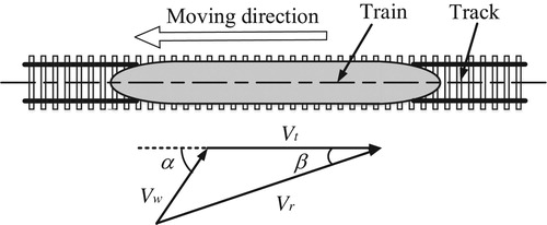
There have been many pieces of research to estimate the aerodynamic behaviors of the train under a crosswind environment using the full-scale experiments, scaled wind tunnel tests and CFD simulations (Alonso-Estébanez, Del Coz Díaz, Álvarez Rabanal, & Pascual-Muñoz, 2017; Baker, Jones, Lopez-Calleja, & Munday, 2004; Gallagher et al., 2018; Niu, Zhou, & Liang, 2018; Suzuki, Tanemoto, & Maeda, 2003). In these investigations, usually the train runs on the flat ground or embankment, and the movement of the train is created by means of the resultant velocity V_r imposed on a static vehicle, as seen in Figure 1, depending on the train speed V_t and incoming wind speed V_w with a wind angle of α. In fact, some studies (Baker, 1986; Suzuki et al., 2003) have indicated that the aerodynamic forces on the train subjected to opening wind environment not only depend on the shape of the vehicle but also can be concerned with that of the different infrastructures where the train travels. For this reason, the aerodynamics of the train running on a bridge may be different from that of other infrastructures. On the other hand, in earlier studies (Bettle, Holloway, & Venart, 2003; Dorigatti et al., 2012) associated with the aerodynamic behaviors of the vehicle-bridge system, the static vehicle model on a bridge was generally adopted as a result of the limitation from the test and calculation technique. In nature, it cannot reflect the real situation due to the aerodynamic interference between train and bridge in the condition of the natural wind, resulting from the moving train. In addition, it is possible that the time-varying aerodynamic loads on the bridge can be observed owing to the changing location of the vehicle. However, one essential reason is that the actual wind velocity on the bridge is the wind speed V_w with a wind angle of α rather than the resultant speed V_r with a yaw angle of β using an equivalent still model. Based on all the problems mentioned above, it is necessary to study and discuss the aerodynamic characteristics of the train-bridge system with a moving train model.

Figure 1. Illustration of resultant velocity on the train.

Generally known, it is difficult and complex to carry out a full-scale experiment to estimate the aerodynamic characteristics of the moving train owing to the unpredictable natural environment, expensive cost and long test period (Baker et al., 2004; Gallagher et al., 2018). For a scaled wind tunnel test in connection with a moving train, Baker (1986) initially developed a moving model rig to explore the forces on the advanced passenger train subjected to an atmospheric boundary layer and then, the train model accelerated by the gravity and traveling along the u-shaped guideway was applied by Bocciolone, Cheli, Corradi, Muggiasca, and Tomasini (2008). In recent years, several servomotor driving devices had been used to create the movement of the vehicle in the scaled experiments (Dorigatti, Sterling, Baker, & Quinn, 2015; Li, Hu, Xu, Zhang, & Liao, 2014; Li, Wang, Xiao, Zou, & Liu, 2018; Xiang, Li, Chen, & Li, 2017). Although some moving models have been devised, there are still many problems to be solved, such as the expensive costs, complex installation, limited train speed. Besides, for the train-bridge system with a moving vehicle, it is not easy to measure the aerodynamic forces on the bridge. At the same time, with the rapid development of computer technology, the CFD approach is also widely approved and adopted in the studies (Alonso-Estébanez et al., 2017; Mosavi, Shamshirband, Salwana, Chau, & Tah, 2019; Niu et al., 2018; Sun, Song, & An, 2012; Yao, Guo, Sun, & Yang, 2015; Zhang, Yu, Zhang, Wu, & Li, 2019), which can better capture the flow characteristics around train-bridge system and easily obtain the aerodynamics affiliated to the train and bridge, compared with a moving vehicle wind tunnel test and full-scale experiment. At present, the dynamic mesh and sliding mesh method are usually used to present the movement of the train in the simulation. Based on the dynamic technique, Wang, Xu, Zhu, and Li (2014) explored the crosswind effect on road vehicles passing by bridge tower and Liu, Chen, Zhou, and Zhang (2018) numerically made an aerodynamic analysis about a train traveling through a rectangular windbreak zone by means of the sliding mesh. Nevertheless, significant disadvantages of these methods are that for the very complex and irregular geometry model of the moving part, it is difficult to generate the solving mesh. So, a new overset mesh is applied in this research to simulate the moving train, which will be demonstrated in Section 2.4.

The main discussions about the train-bridge system in the above investigations concentrate on the aerodynamic behaviors of the train rather than that of the bridge because it is not easy to measure the aerodynamic loads acting on the bridge. Actually, Li, Wang, Xu, and Liao (2011) pointed out that the interactions resulting from the moving train and air, have significant impacts on the flow around the bridge, which can change the flow characteristics of the bridge such as the velocity, pressure, streamline, and the similar results were demonstrated in the paper by Yao, Zhang, Xia, and Li (2018). Based on the researches above, more details of aerodynamic performances of the train-bridge system should be investigated and analyzed under an opening crosswind condition.

This paper is organized as follows. In Section 2, the brief details about the simulated model including the numerical method, flow domain, corresponding boundary condition, geometry and meshes are given. Besides, the aerodynamic coefficients using overset mesh method are compared with that of the wind tunnel test to validate the accuracy of the mesh and numerical algorithm. Then, Section 3 shows the flow and the aerodynamic loads of train and bridge in more details with a range of the varying running speeds and incoming wind speeds. Specifically, Section 3.1 expresses the aerodynamic interaction between the moving train and crosswind in terms of the flow features around the train-bridge system at the varying yaw angles, and the effect of moving train on the aerodynamic forces of the train and bridge including the side force, lift force and rolling moment are demonstrated and analyzed in Section 3.2. Finally, some broad conclusions and further works are summarized in Section 4.

2. Methodology

2.1. Computational method

The flow around the train-bridge system under a crosswind is a variably complicated three- dimensional turbulent, and accurate prediction of turbulent flow is a problem that has not been solved satisfactorily so far. In this study, the Reynolds-Average Navier-Stokes (RANS) equation, based on three- dimensional incompressible flow, is utilized. The shear stress transport (SST) turbulence model based on k-ω relationship is adopted to consider the transmission of shear stress in turbulent flow.

2.2. Flow domain and boundary conditions

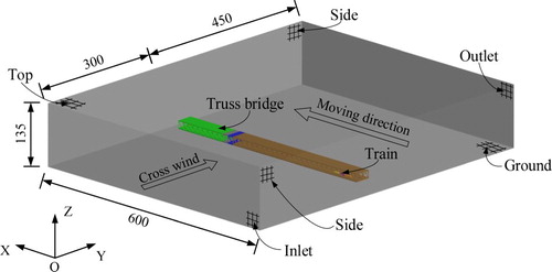
The model is established in full-scale dimensions. In order to capture the real flow field around train and bridge, and minimize the boundary effect in crosswinds, a large enough computational domain of fluid should be considered, the key dimensions of which are reported in Figure 2. The spatial flow domain is 750 m in length, 600 m in width and 135 m in height, in which the upstream length of the domain is set as 300 m while the downstream length as 450 m due to the flow difference between the upstream and downstream. A uniform velocity boundary condition with the turbulence intensity of 5% is adopted, and the pressure outlet boundary is imposed a gauge zero pressure on the outlet of the flow zone. For the ground and the external surface of train and bridge, a no-slip wall and standard wall function are used to perform the wall effect. The top and side surfaces of the flow zone are set as slip walls boundary condition.

Figure 2. Computational domain of fluid and boundary condition (unit: m).

2.3. Geometry model and mesh

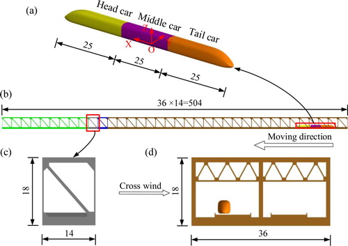
The numerical computation of a complete high-speed train with a length about 200 m is out of available computing resources by a great deal at present and for this reason, the flow around train with some simplifications, ignoring wheel set, mirrors, windshield wipers and other attached parts, is calculated in this work. Investigated from the previous research by Cooper (1984), it is found that a decrease in length of train does not change the flow behavior around train if the length remains above the limit suggested by him. Accordingly, the total length of train including a head-car, a middle-car and a tail-car, is 75 m, as illustrated in Figure 3(a). The steel truss bridge model consisting of 36 segments with 14 m in length, 36 m in width and 18 m in height is shown in Figure 3(b), which comes from a real long-span cable-stayed bridge under construction across the Yangtze River near the estuary to the East China Sea. The track, ballast and other details on the bridge are neglected as well.

Figure 3. Geometry model (unit: m): (a) train model details; (b) side view of overall layout; (c) a segment of bridge model; (d) front view of overall layout.

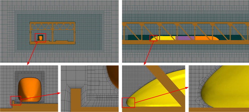
The hexahedral dominated cell meshing technique is employed to discretize the computational domain. A finer resolution is required closed to the surface of train and bridge in order to correctly reproduce the geometrical details and to better capture the flow features, and the minimum cell size is set to 5 mm on the train surface, as shown in Figure 4. While a coarser cell is adopted far from the train and bridge zone where the flow is less perturbed and the turbulence effect is less important (Cheli, Ripamonti, Rocchi, & Tomasini, 2010). Some researches (Baker, 2010; Sterling, Baker, Jordan, & Johnson, 2008) reveal that the flow around train can be affected by the thickness of boundary layer and the corresponding y+ value is 30–120 in order to meet the requirement of the standard wall function used in the case. The finest boundary mesh in the surface of train and bridge is created to 1 mm, and the total cells number is about 20 million in the model.

Figure 4. Meshes around the train.

2.4. Overset mesh

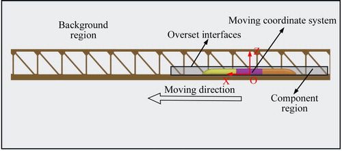
The overset mesh method is applied to present the relative motion between the train and bridge in the simulation. Overset mesh, also called ‘Chimera’ or overlapping methodology is especially useful in problems dealing with multiple or moving parts, as well as optimization studies. The cases involving overset mesh have a background mesh enclosing the entire flow domain and one or more component mesh containing the moving bodies within the domain. It should be noted that, compared to remeshing or sliding mesh method, an advantage of overset mesh is that the individual mesh, including the background region and component region, can be generated independently with fewer constraints, which is especially applicable for some complex and irregular moving bodies in the flow. In this case, the computational domain is divided into two subdomains: a stationary outer subdomain (background region) including the truss bridge, and a moving subdomain (component region) including the train with a volume of air around it, as illustrated in Figure 5. For overset meshing to be successful, there is sufficient overlap between background and component regions. Overset interfaces are created in the overlapping surfaces to connect the background zone and component zone by interpolating cell data in the overlapping boundary condition. A moving coordinate system is established in the component region to create the motion of the train and meanwhile, the overset interfaces coming from overlapping in subdomain are continually updated with the moving train.

Figure 5. Overview of overset mesh.

2.5. CFD validation

The CFD results are compared with the results from a 1/30 scaled wind tunnel tests carried out by Li et al. (2018) to validate the accuracy of this numerical model. The all experimental settings in wind tunnel tests are also identically used in the validation case. A lot of related studies (Dorigatti et al., 2015; Premoli, Rocchi, Schito, & Tomasini, 2016) show that the aerodynamic loads of the train are only depend on the resultant wind velocity as a result of the combination of train speed and incoming wind velocity. With reference to Figure 1, the actual resultant wind speed V_r with a yaw angle β on the train, is straightforward to be obtained from the following expressions: (1) $\begin{array}{rl}{V}_w^{\mathrm{\prime }}& =V_w\sin \alpha ;V_t^{\mathrm{\prime }}=V_t+V_w\cos \alpha \end{array}$(1) (2) $\begin{array}{rl}{V_r}^2& =V_t^{\mathrm{\prime }2}+V_w^{\mathrm{\prime }2}\end{array}$(2) (3) $\begin{array}{rl}\tan \beta & =V_w^{\mathrm{\prime }}/V_t^{\mathrm{\prime }}\end{array}$(3)

The definition of aerodynamic coefficients remains consistent with the test. The mean side load, lift load, and rolling moment coefficients can be expressed as follows: (4) $\begin{array}{rl}{C}_S& =F_y/(\frac{1}{2}\rho {V_r}^{2}A)=F_S/(\frac{1}{2}\rho {V_r}^{2}A)\\ C_L& =F_z/(\frac{1}{2}\rho {V_r}^{2}A)=F_L/(\frac{1}{2}\rho {V_r}^{2}A)\\ C_R& =M_x/(\frac{1}{2}\rho {V_r}^{2}Ah)=M_R/(\frac{1}{2}\rho {V_r}^{2}Ah)\end{array}$(4) where C_S is the side load coefficient; C_L is the lift load coefficient; C_R is the rolling moment coefficient; F_S is the side force; F_L is the lift force; M_R is the rolling moment; V_r is the wind speed relative to the train; ρ is the air density; A is the side area of the car; and h is the height of the car.

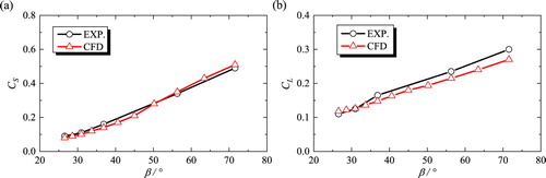
It can be obtained from Figure 6 that the curves of C_S and C_L coefficients created by the different yaw angles are in good agreement between the experimental and numerical data. It should be noted that there is a greater difference in C_L coefficient than in the C_S coefficient, which may be caused by the high stochastic turbulence produced by truss bridge in crosswinds. In fact, the lift force can be easily affected by wind characteristics underneath the train (Zhang, Li, Tian, Gao, & Sheridan, 2016) and the complete agreement of the results cannot be expected for the flows because the flow is turbulent. The maximum error between the simulation and test is less than 10%, which implies the numerical results are an acceptable agreement in engineering application.

Figure 6. Comparison between simulation and test: (a) side force coefficient; (b) lift force coefficient.

3. Results and discussion

3.1. Flow features

3.1.1. Flow around the train

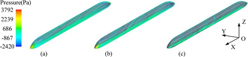
To better exhibit the flow around train exposed to natural wind, the surface pressure contour of the train is demonstrated in Figure 7. The aerodynamic performances of train on the windward side and the leeward side are obviously different. It is visible that a high-pressure region is generated on the windward side of the train, while a low-pressure region on all other sides. In addition, it can be observed that a significant difference, the positive pressure reducing on the windward flank and the negative pressure increasing on the leeward flank, exists along the traveling direction from the front to rear, which may be produced by the interaction of the moving train and incoming wind. Clearly the extreme pressure obtained at stagnation point, appears on the nose of head-car due to the compressible effect of moving train on the air, while the lower pressure is given on the top and bottom of tail-car, perhaps indicating some separated flow in this region. It is worth remarking that the shielding effect of web member of truss bridge is depicted on the pressure distribution of windward side.

Figure 7. Illustration of surface pressure on the train (β = 35.75°, V_t = 100 km/h, V_w = 20 m/s, α = 90°): (a) three- dimensional surface pressure; (b) pressure distribution of the different surfaces.

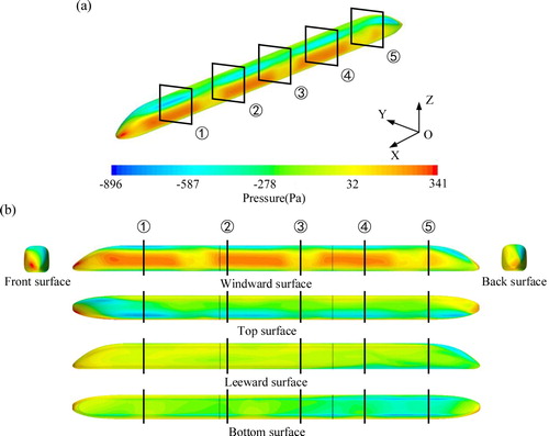
In order to better explore these differences, an additional comparison is reported in terms of surface pressure distribution for different train sections, as seen in Figure 8. It is possible to see that there are higher suctions on the windward roof and base corner, smaller suctions over the rest of the roof, leeward side and underbody. The same results were described in previous experiment and computational investigations (Baker, 2010; Chiu, 1995; Wang, Li, Xiao, Zou, & Sha, 2018b). Near the nose, a larger pressure variation between windward and leeward is obtained, which can be expected to give a major contribution to the side force, however, there is a lower pressure difference for the sections near the tail-car. For the suction peak, it gradually decreases from locomotive to caboose, neglecting the shelter from the web member. Note that the shielding effect from the web member, demonstrated in section $◯3$, produces a smaller suction in comparison with other sections.

Figure 8. Surface pressure distribution at different train sections (β = 35.75°, V_t = 100 km/h, V_w = 20 m/s, α = 90°, unit: Pa): (a) section $◯1$; (b) section $◯2$; (c) section $◯3$; (d) section $◯4$; (e) section $◯5$.

The flow pattern on the surface of train at different yaw angles is performed by the form of surface streamlines filled in pressure, sketched in Figure 9. The results reveal that the flow begins to detach from the leading nose to the tail of the train. As approaching the exposed large angles, a larger separation angle is apparently observed on the top of the train, which indicates the flow around the train is characterized by three-dimensional structures that mainly result from the combination between natural wind and train-induced wind on the zone of train nose. The flow, blowing over the train nose and detaching from the windward roof corner, is deflected along the train axis with a certain angle. It can be deduced that the larger yaw angle mainly dominated by the incoming wind velocity can produce a larger flow separation and lead to more complex three-dimensional flow around the train.

Figure 9. Surface streamlines on the train filled in pressure at different yaw angles: (a) β = 6.08°, V_t = 300 km/h, V_w = 10 m/s, α = 90°; (b) β = 13.50°, V_t = 300 km/h, V_w = 20 m/s, α = 90°; (c) β = 35.75°, V_t = 100 km/h, V_w = 20 m/s, α = 90°.

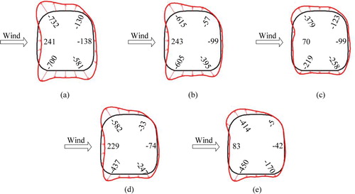
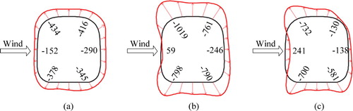
To analyze the aerodynamic effect of the transverse wind and train induced wind, more detailed pressure distribution on the train for section $◯1$ at the varying yaw angles is reported in Figure 10. It is clearly seen that the resultant yaw angles are possible to change the flow field, and the most of suctions focus on the flow separation zone, which is the windward roof and base corner. At higher yaw angle, the pressure on the windward side becomes greater, while on the lee side it is smaller. In general, the pressure difference between them becomes larger, which means larger yaw angle can contribute to higher side force. The extreme suction depends not only on resultant wind direction β, but also on relative wind speed V_r.

Figure 10. Surface pressure distribution at different yaw angles for section $◯1$ (unit: Pa): (a) β = 6.08°, V_t = 300 km/h, V_w = 10 m/s, α = 90°; (b) β = 13.50°, V_t = 300 km/h, V_w = 20 m/s, α = 90°; (c) β = 35.75°, V_t = 100 km/h, V_w = 20 m/s, α = 90°.

These discussions above suggest that, for a train traveling on the truss bridge, the main flow features around train are similar to that on the ground or embankment, but it also can be affected by the infrastructures where the train runs. Meanwhile, the varying yaw angles also play a significant role in flow structures of the train.

3.1.2. Flow around the bridge

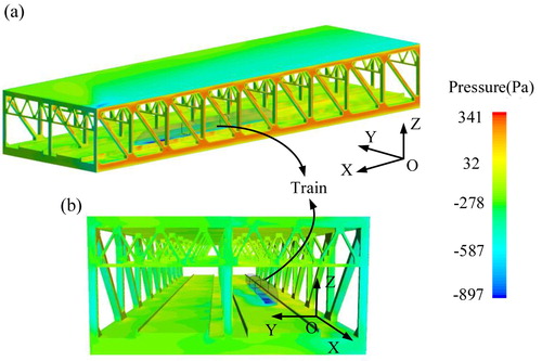
For the truss bridge, seen in Figure 11(a), a pressure distribution similar to that of the train can be observed: a high-pressure zone mainly appears on the windward side and a lower pressure zone on the other sides. The aerodynamic effect of moving train is presented in terms of the distinct suction area where the pressure decreases along the traveling direction of the train, reported in Figure 11(b). It is worth noting that the location of train is constantly changing, so the pressure distribution on the deck of bridge also varies with the time, which can lead to the time-varying aerodynamic forces on the bridge.

Figure 11. Surface pressure on the bridge (β = 35.75°, V_t = 100 km/h, V_w = 20 m/s, α = 0°): (a) three- dimensional surface pressure distribution; (b) front surface pressure distribution.

3.2. Aerodynamic loads

Hereinafter, the aerodynamic forces on the train and bridge under a crosswind are discussed. In the analysis, the aerodynamic forces come from the sum of the pressure difference and viscous, and act on the centroid of structure. To ensure the train running within the fully-developed flow field, the aerodynamic loads are obtained after the train moves to a certain distance.

3.2.1. Aerodynamic forces on the train

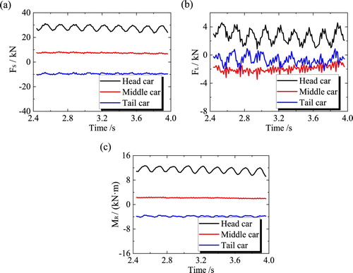
The time-varying aerodynamic forces of the cars are illustrated in Figure 12. It shows that the forces on the head-car are larger than those of middle-car and tail-car. In the light of previous analysis, it may be caused by the flow separation on the nose of head- car to change the flow structure around the train, due to the combination between crosswind and moving train. The results suggest that there may be a larger operational risk in the head-car when a train travels with a high speed related to nature wind (Guo, Xu, Xia, Zhang, & Shum, 2007; Zhai et al., 2015). It is worth mentioning that the time-varying curve of rolling moment is similar to that of side force, which means the rolling moment mainly comes from the contribution of side force. Moreover, the periodic fluctuating loads on the train dramatically highlighted on the head car, are visibly demonstrated as a result of the shielding effect of web member of the bridge.

Figure 12. Aerodynamic force curves of each car (β = 35.75°, V_t = 100 km/h, V_w = 20 m/s, α = 90°): (a) side force; (b) lift force; (c) rolling moment.

In previous researches (Baker, 2010; Cheli et al., 2010), it is confirmed that the aerodynamic loads acting on the structure induced by wind can be expressed by the corresponding non-dimensional coefficient, remaining the same direction with the wind and only depending on the shape of the structure at a certain Reynolds number. Therefore, the non-dimensional aerodynamic coefficients, defined by Equation (3), are adopted to describe the aerodynamic forces in the most investigations in crosswinds. However, the coefficients only show the ultimate effect in a condition of the train-induced wind and cross wind and the individual contribution resulting from the moving train, incoming wind and the mutual influence between them cannot be presented. For this reason, we can approximately make a basic assumption that the aerodynamic forces on the train are redefined as (5) $\begin{array}{r}F=\frac{1}{2}\rho A(a{V}_t^{\mathrm{\prime }2}+b{V}_t^{\mathrm{\prime }}{V}_w^{\mathrm{\prime }}+c{V}_w^{\mathrm{\prime }2})\end{array}$(5) Where, a, b and c are three constant coefficients, respectively, obtained from fitting curve; the $a{V}_t^{\mathrm{\prime }2}$ and $c{V}_w^{\mathrm{\prime }2}$ respectively represent the contribution from moving train and crosswind; and the $b{V}_t^{\mathrm{\prime }}{V}_w^{\mathrm{\prime }}$ indicates the interaction between them. Considering the Equations (3) and (5), the aerodynamic force can be written as the following forms: (6) $\begin{array}{rl}F& =\frac{1}{2}\rho A{V}_w^{\mathrm{\prime }2}\left(a{\left(\frac{{V^{\mathrm{\prime }}}_t}{{V^{\mathrm{\prime }}}_w}\right)}^2+b\frac{{V^{\mathrm{\prime }}}_t}{{V^{\mathrm{\prime }}}_w}+c\right)\\ & =\frac{1}{2}\rho A{V}_w^{\mathrm{\prime }2}(a{\left(\frac{1}{\tan \beta }\right)}^2+b\frac{1}{\tan \beta }+c)\\ & =\frac{1}{2}\rho A{C}^{\mathrm{\prime }}{V}_w^{\mathrm{\prime }2}\end{array}$(6) (7) $\begin{array}{rl}{C}^{\mathrm{\prime }}& =a{\left(\frac{1}{\tan \beta }\right)}^2+b\frac{1}{\tan \beta }+c\end{array}$(7) Where C^’ is another aerodynamic coefficient as a function of the resultant wind angle β.

Figure 13 depicts the aerodynamic coefficients calculated by Equation (7), and the fitting curve is created by the varying yaw angles. It should be mentioned that the rolling moment is not discussed because the developing law is similar to that of the side forces, reported in Figure 12. In this diagram, the fitting curves of aerodynamic coefficients are in good agreement with the data obtained in simulation. The side coefficients of head-car and tail-car significantly decrease with the improving yaw angle, while the lift coefficient increases. For the coefficients of middle-car, there are no evident variation due to the quite steady flow around it. In the condition of lower angle, the coefficients on the head-car and tail-car are sensitive to the different yaw angles owing to the effect of moving train.

Figure 13. Fitting curves of aerodynamic coefficients of each car at different yaw angles β: (a) side force coefficients; (b) lift force coefficients.

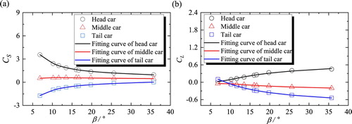
The fitting coefficients are performed in more details in Tables 1 and 2, giving the proportion of each component including the train speed, wind speed and interaction between them for aerodynamic loads. It can be seen from this tables that, at a lower yaw angle 0–20°, the side force is mainly governed by the combination that comes from the moving train and incoming wind, but when the yaw angle ranges toward higher, the transverse wind can make more contribution, which shows the influence of moving train for the side force is only represented at the lower yaw angle and the same results are found in lift force.

Table 1. The fitting coefficients of aerodynamic forces.

	Fitting coefficients of side forces			Fitting coefficients of lift forces
Car body	aS	bS	cS	aL	bL	cL
Head car	0.01150	0.26653	0.56457	0.00901	−0.15295	0.66630
Middle car	−0.00900	0.09333	0.35495	−0.00469	0.06776	−0.28587
Tail car	−0.00238	−0.22757	0.33640	−0.00730	0.16417	−0.75634

Table 2. The proportion of moving train, cross wind and interaction between them for aerodynamic forces at different yaw angles.

	Side force			Lift force
Yaw angle β /°	Train speed	Interaction	Wind speed	Train speed	Interaction	Wind speed
6.84	0.22	0.62	0.16	35.94	−73.21	38.27
10.20	0.15	0.62	0.24	2.94	−8.98	7.04
11.62	0.13	0.61	0.26	1.57	−5.48	4.91
13.50	0.11	0.59	0.30	0.84	−3.44	3.59
16.07	0.09	0.57	0.35	0.45	−2.18	2.73
16.70	0.08	0.56	0.36	0.39	−1.99	2.60
19.80	0.06	0.53	0.41	0.22	−1.37	2.14
25.64	0.04	0.47	0.48	0.10	−0.82	1.72
35.75	0.02	0.39	0.59	0.04	−0.45	1.41

3.2.2. Aerodynamic forces on the bridge

In general, for the long span truss bridge composed of many identical segments, the aerodynamic loads acting on one of the segments are investigated, seen in Figure 3(c), to make a further dynamic analysis on train-bridge system under a crosswind environment (Guo et al., 2007; Li et al., 2005; Xia et al., 2008). Figure 14 draws the data graph of aerodynamic forces on the monitored segment exposure to different wind speeds and running speeds. To better research the differences in the aerodynamic forces as a result of the moving train, it should be mentioned that the abscissa in these figures is coordinated by means of the moving distance of train instead of the time. It is apparent from this graphs that noticeable changes of the aerodynamic forces in the process of the train driving into and out of the bridge, especially the lift force and rolling moment, are observed. When the train body passes the monitored segment at a constant speed, the forces keep relatively stable regardless of a little fluctuation. Referring to previous studies (Niu et al., 2018; Wang et al., 2018a), the variation trend is similar to that of the pressure wave induced by the moving train. When the train travels with a high speed, the air in the front of the head car will be compressed and diffuses around, but the bridge deck can block the diffusing air to change the pressure distribution on the surface. On the other hand, with the train leaving the bridge, the space occupied by the moving train will be again filled with airs, which is also able to change the flow around the deck to produce a complex wake (Baker, 2010; Sun et al., 2012; Yao et al., 2013). That can explain the distinct changes of the aerodynamic forces on the bridge.

Figure 14. Aerodynamic force curves of the bridge at different wind speeds and train speeds: (a), (b) and (c) show the forces curves at different wind speeds with 300 km/h train speed respectively; (d) (e) and (f) show the forces curves at different train speeds with 20 m/s wind speed respectively.

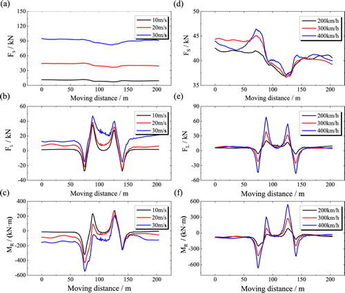
From Figure 14 one can see that with the improving wind speed, the side force significantly increases, while for the lift force, wind speed can affect the amplitude of loads but not obviously and the variation of rolling moment comes from the collective contribution of the side force and lift force. The effect of wind speed on the aerodynamic loads can be seen in Figure 15, expressed by the mean forces. It is apparent that the growing wind speed increases the mean aerodynamic loads. From previous researches (Holmes, 2001), one can see that for the flow under crosswinds, the time-averaged aerodynamic loads have a linear relationship with the squared wind speed and Table 3 lists more detailed results about aerodynamic loads. It is found that the ratio of mean force to squared wind velocity is close to a constant, regardless of the error from the unsteady turbulent flow. It can be induced that the mean aerodynamic loads are proportional to the squared wind velocity.

Figure 15. The mean aerodynamic forces on the bridge: (a) different wind speeds with 300 km/h train speed; (b) different train speeds with 20 m/s wind speed.

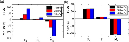
Table 3. The mean aerodynamic forces on the bridge at different wind speeds.

	Side force		Lift force		Rolling moment
Wind speed Vw/(m/s)	FS/kN	FS/$V_w^2$	FL/kN	FL/$V_w^2$	MR/(kN·m)	MR/$V_w^2$
10	9.56	95.60	1.66	16.60	−14.42	−144.20
20	41.41	103.53	6.41	16.03	−61.26	−153.15
30	90.07	100.08	16.04	17.82	−134.18	−149.09

As seen in Figure 14(d), the increasing train speed has no obvious influence on side force, while for the lift force and rolling moment, the maximum and minimum peaks significantly improves, as illustrated in Figure 14(e,f). According to Figure 15(b) and Table 4, the mean aerodynamic loads are not affected by the varying running speed. Prior studies (Tian, 2007) showed that the amplitude variation in force induced by the moving train can be stated with a quadratic function of train speed. Based on this, in this study, the sudden variation of aerodynamic forces is used to analyze the effect of moving train on aerodynamic loads of bridge, as demonstrated in Tables 5 and 6. The results show clearly that the varying crosswind speed has little impact on the sharp magnitude of aerodynamic forces, but it is noticeable from Table 6 that the magnitudes of aerodynamic load, particularly for the lift force and rolling moment, remain an approximately linear dependence with the squared train speed. For the side fore, it is worth remarking that the increasing train speed improves the sudden change but it is not a linear function of the squared train speed. The main reason for this phenomenon may be that the moving train can only affect the pressure distribution on the bridge deck rather than that of side surface.

Table 4. The mean aerodynamic forces on the bridge at different train speeds with 20 m/s wind speed.

Train speed/(km/h)	Side force FS/kN	Lift force FL/kN	Rolling moment MR/(kN·m)
200	40.46	6.86	−65.11
300	41.41	6.41	−64.26
400	41.55	6.93	−65.26

Table 5. The sudden variation of aerodynamic forces on the bridge at different wind speeds.

Wind speed/(m/s)	Side force ΔFS/kN	Lift force ΔFL/kN	Rolling moment ΔMR/(kN·m)
10	5.44	62.16	552.44
20	5.60	60.54	525.46
30	5.86	62.15	537.02

Table 6. The sudden variation of aerodynamic forces on the bridge at different train speeds.

	Side force		Lift force		Rolling moment
Train speed/ (km/h)	ΔFS/kN	ΔFS/$V_t^2$	ΔFL/kN	ΔFL/$V_t^2$	ΔMR/(kN·m)	ΔMR/$V_t^2$
200	3.69	1.20	26.56	8.61	233.02	72.50
300	5.80	0.84	60.54	8.72	525.46	75.67
400	6.58	0.53	110.37	8.94	968.17	78.42

4. Conclusions and future work

When a train travels on a bridge at a high speed, the train-induced wind and the cross wind are combined to form a complicated interaction, which has a crucial impact on the flow around train-bridge system. In this study, the aerodynamic characteristics associated with the train and bridge with a crosswind are investigated using a new overset mesh technique and it is found that the numerical calculations in comparison with the previous wind tunnel test are reliable. Furthermore, a fitting formula for a variety of yaw angles is developed to predict the aerodynamic forces. The main conclusions are drawn as follows:

1. Under a crosswind environment, the major aerodynamic features relative to a moving train are similar to that on the ground or embankment, mainly depending on the resultant speed V_r and the resultant yaw angle β, but it also can be affected by the different infrastructures where the train travels. A high-pressure region is observed on the nose of head-car, while a low-pressure region on tail of the train as a result of the effect of moving train.

2. The aerodynamic interaction from the moving train and cross wind can change the flow around the train-bridge system to produce larger aerodynamic forces on the head-car in comparison with the middle- and tail-car, which means the head-car may be subjected to more running risks. At lower yaw angles of 0–20°, the aerodynamic forces mainly result from the contribution of moving train and the combination of train speed and wind speed. While at higher yaw angles ranging from 20° to 40°, the incoming wind velocity plays a key role in the aerodynamic forces. Besides, the shielding effect from web member of the truss is demonstrated in terms of the periodic fluctuating loads on the car-body.

3. For the bridge, in the process of the train entering and leaving, the sudden variations of aerodynamic loads are obtained due to the varying pressure distribution on the deck caused by the moving train. The mean aerodynamic forces are independent with the traveling speed, but it is approximate a linear function with the square of the incoming wind speed. On the other hand, for the lift force and rolling moment, the sharp variations are directly proportional to the squared train speed.

4. It should be noted that the results, including the flow characteristics and aerodynamic forces of the train-bridge system, are only applicable for the high-speed train on a truss bridge in this research, so more study cases for different types of trains and bridges should be investigated to validate the general conclusions and observations in further works. Also, the dynamic analysis of the train-bridge system under a wind action is necessary to be carried out to improve the running performance and stability of the railway vehicles and to optimize the aerodynamic performances of the train in the future.

Disclosure statement

No potential conflict of interest was reported by the authors.

Additional information

Funding

This work was accomplished by the supports of the Fundamental Research Funds for the Central Universities [grant number 2017YJS150]; the National Natural Science Foundation of China [grant number 51720105005], the 111 Project [grant number B13002] and the program of China Scholarships Council [grant number 201807090042].

References

- Alonso-Estébanez, A., Del Coz Díaz, J. J., Álvarez Rabanal, F. P., & Pascual-Muñoz, P. (2017). Numerical simulation of bus aerodynamics on several classes of bridge decks. Engineering Applications of Computational Fluid Mechanics, 11(1), 435–449. doi: 10.1080/19942060.2016.1201544
- Baker, C. J. (1986). Train aerodynamic forces and moments from moving model experiments. Journal of Wind Engineering and Industrial Aerodynamics, 24(3), 227–251. doi: 10.1016/0167-6105(86)90024-3
- Baker, C. J. (2010). The flow around high speed trains. Journal of Wind Engineering and Industrial Aerodynamics, 98(6–7), 277–298. doi: 10.1016/j.jweia.2009.11.002
- Baker, C. J., Jones, J., Lopez-Calleja, F., & Munday, J. (2004). Measurements of the cross wind forces on trains. Journal of Wind Engineering and Industrial Aerodynamics, 92(7–8), 547–563. doi: 10.1016/j.jweia.2004.03.002
- Bettle, J., Holloway, A. G. L., & Venart, J. E. S. (2003). A computational study of the aerodynamic forces acting on a tractor-trailer vehicle on a bridge in cross-wind. Journal of Wind Engineering and Industrial Aerodynamics, 91(5), 573–592. doi: 10.1016/S0167-6105(02)00461-0
- Bocciolone, M., Cheli, F., Corradi, R., Muggiasca, S., & Tomasini, G. (2008). Crosswind action on rail vehicles: Wind tunnel experimental analyses. Journal of Wind Engineering and Industrial Aerodynamics, 96(5), 584–610. doi: 10.1016/j.jweia.2008.02.030
- Cai, C., Hu, J. X., Chen, S., Zhang, W., & Kong, X. (2015). A coupled wind-vehicle-bridge system and its applications: A review. Wind and Structures, 20(2), 117–142. doi: 10.12989/was.2015.20.2.117
- Cheli, F., Ripamonti, F., Rocchi, D., & Tomasini, G. (2010). Aerodynamic behaviour investigation of the new EMUV250 train to cross wind. Journal of Wind Engineering and Industrial Aerodynamics, 98(4–5), 189–201. doi: 10.1016/j.jweia.2009.10.015
- Chiu, T. W. (1995). Prediction of the aerodynamic loads on a railway train in a cross-wind at large yaw angles using an integrated two- and three-dimensional source/vortex panel method. Journal of Wind Engineering and Industrial Aerodynamics, 57(1), 19–39. doi: 10.1016/0167-6105(94)00099-Y
- Cooper, R. K. (1984). Atmospheric turbulence with respect to moving ground vehicles. Journal of Wind Engineering and Industrial Aerodynamics, 17(2), 215–238. doi: 10.1016/0167-6105(84)90057-6
- Dorigatti, F., Sterling, M., Baker, C. J., & Quinn, A. D. (2015). Crosswind effects on the stability of a model passenger train-A comparison of static and moving experiments. Journal of Wind Engineering and Industrial Aerodynamics, 138, 36–51. doi: 10.1016/j.jweia.2014.11.009
- Dorigatti, F., Sterling, M., Rocchi, D., Belloli, M., Quinn, A. D., Baker, C. J., & Ozkan, E. (2012). Wind tunnel measurements of crosswind loads on high sided vehicles over long span bridges. Journal of Wind Engineering and Industrial Aerodynamics, 107–108, 214–224. doi: 10.1016/j.jweia.2012.04.017
- Gallagher, M., Morden, J., Baker, C., Soper, D., Quinn, A., Hemida, H., & Sterling, M. (2018). Trains in crosswinds – comparison of full-scale on-train measurements, physical model tests and CFD calculations. Journal of Wind Engineering and Industrial Aerodynamics, 175(December 2017), 428–444. doi: 10.1016/j.jweia.2018.03.002
- Guo, W. W., Xu, Y. L., Xia, H., Zhang, W. S., & Shum, K. M. (2007). Dynamic response of suspension bridge to typhoon and trains. II: Numerical results. Journal of Structural Engineering, 133(1), 12–21. doi:10.1061/(ASCE)0733-9445(2007)133:1(12)
- Holmes, J. D. (2001). Wind loading of structures. London: Spon Press.
- Li, Y., Hu, P., Xu, Y., Zhang, M., & Liao, H. (2014). Wind loads on a moving vehicle-bridge deck system by wind-tunnel model test. Wind and Structures, 19(2), doi: 10.12989/was.2014.19.2.145
- Li, Y., Qiang, S., Liao, H., & Xu, Y. L. (2005). Dynamics of wind-rail vehicle-bridge systems. Journal of Wind Engineering and Industrial Aerodynamics, 93(6), 483–507. doi: 10.1016/j.jweia.2005.04.001
- Li, X. Z., Wang, M., Xiao, J., Zou, Q. Y., & Liu, D. J. (2018). Experimental study on aerodynamic characteristics of high-speed train on a truss bridge: A moving model test. Journal of Wind Engineering and Industrial Aerodynamics, 179, 26–38. doi: 10.1016/j.jweia.2018.05.012
- Li, Y., Wang, B., Xu, Y., & Liao, H. (2011). Numerical simulation of aerodynamic characteristics for static and dynamic vehicle-bridge system under cross wind. China Civil Engineering Journal, 44(1), 87–94. (in Chinese) doi: 10.15951/j.tmgcxb.2011.s1.016
- Liu, T., Chen, Z., Zhou, X., & Zhang, J. (2018). A CFD analysis of the aerodynamics of a highspeed train passing through a windbreak transition under crosswind. Engineering Applications of Computational Fluid Mechanics, 12(1), 137–151. doi: 10.1080/19942060.2017.1360211
- Mosavi, A., Shamshirband, S., Salwana, E., Chau, K., & Tah, J. H. M. (2019). Prediction of multi-inputs bubble column reactor using a novel hybrid model of computational fluid dynamics and machine learning. Engineering Applications of Computational Fluid Mechanics, 13(1), 482–492. doi: 10.1080/19942060.2019.1613448
- Niu, J., Zhou, D., & Liang, X. (2018). Numerical investigation of the aerodynamic characteristics of high-speed trains of different lengths under crosswind with or without windbreaks. Engineering Applications of Computational Fluid Mechanics, 12(1), 195–215. doi: 10.1080/19942060.2017.1390786
- Premoli, A., Rocchi, D., Schito, P., & Tomasini, G. (2016). Comparison between steady and moving railway vehicles subjected to crosswind by CFD analysis. Journal of Wind Engineering and Industrial Aerodynamics, 156, 29–40. doi: 10.1016/j.jweia.2016.07.006
- Sterling, M., Baker, C. J., Jordan, S. C., & Johnson, T. (2008). A study of the slipstreams of high-speed passenger trains and freight trains. Proceedings of the Institution of Mechanical Engineers, Part F: Journal of Rail and Rapid Transit, 222(2), 177–193. doi: 10.1243/09544097JRRT133
- Sun, Z., Song, J., & An, Y. (2012). Numerical simulation of aerodynamic noise generated by high speed. Engineering Applications of Computational Fluid Mechanics, 6(2), 173–185. doi: 10.1080/19942060.2012.11015412
- Suzuki, M., Tanemoto, K., & Maeda, T. (2003). Aerodynamic characteristics of train/vehicles under cross winds. Journal of Wind Engineering and Industrial Aerodynamics, 91(1–2), 209–218. doi: 10.1016/S0167-6105(02)00346-X
- Thomas, D., Diedrichs, B., Berg, M., & Stichel, S. (2010). Dynamics of a high-speed rail vehicle negotiating curves at unsteady crosswind. Proceedings of the Institution of Mechanical Engineers, Part F: Journal of Rail and Rapid Transit, 224(6), 567–579. doi: 10.1243/09544097JRRT335
- Tian, H. (2007). Train aerodynamics. Beijing: China Railway Press. (in Chinese)
- Wang, M., Li, X. Z., Xiao, J., Zou, Q. Y., & Sha, H. Q. (2018b). An experimental analysis of the aerodynamic characteristics of a high-speed train on a bridge under crosswinds. Journal of Wind Engineering and Industrial Aerodynamics, 177, 92–100. doi: 10.1016/j.jweia.2018.03.021
- Wang, Y., Xia, H., Guo, W., Zhang, N., & Wang, S. (2018a). Numerical analysis of wind field induced by moving train on HSR bridge subjected to crosswind. Wind and Structures, 27(1), 29–40. doi: 10.12989/was.2018.27.1.029
- Wang, B., Xu, Y. L., Zhu, L. D., & Li, Y. L. (2014). Crosswind effect studies on road vehicle passing by bridge tower using computational fluid dynamics. Engineering Applications of Computational Fluid Mechanics, 8(3), 330–344. doi: 10.1080/19942060.2014.11015519
- Xia, H., Guo, W. W., Zhang, N., & Sun, G. J. (2008). Dynamic analysis of a train-bridge system under wind action. Computers and Structures, 86(19–20), 1845–1855. doi: 10.1016/j.compstruc.2008.04.007
- Xiang, H., Li, Y., Chen, S., & Li, C. (2017). A wind tunnel test method on aerodynamic characteristics of moving vehicles under crosswinds. Journal of Wind Engineering and Industrial Aerodynamics, 163, 15–23. doi: 10.1016/j.jweia.2017.01.013
- Yao, S., Guo, D., Sun, Z., & Yang, G. (2015). A modified multi-objective sorting particle swarm optimization and its application to the design of the nose shape of a high-speed train. Engineering Applications of Computational Fluid Mechanics, 9(1), 513–527. doi: 10.1080/19942060.2015.1061557
- Yao, S., Sun, Z., Guo, D., Chen, D., & Yang, G. (2013). Numerical study on wake characteristics of high-speed trains. Acta Mechanica Sinica, 29(6), 811–822. doi: 10.1007/s10409-013-0077-3
- Yao, Z., Zhang, N., Xia, H., & Li, X. (2018). Study on aerodynamic performance of three-dimensional train-bridge system based on overset mesh. Engineering Mechanics, 35, 38–46. (in Chinese) doi: 10.6052/j.issn.1000-4750.2017.03.0254
- Zhai, W., Yang, J., Li, Z., & Han, H. (2015). Dynamics of high-speed train in crosswinds based on an air-train-track interaction model. Wind and Structures, 20(2), 143–168. doi: 10.12989/was.2015.20.2.143
- Zhang, J., Li, J., Tian, H., Gao, G., & Sheridan, J. (2016). Impact of ground and wheel boundary conditions on numerical simulation of the high-speed train aerodynamic performance. Journal of Fluids and Structures, 61, 249–261. doi: 10.1016/j.jfluidstructs.2015.10.006
- Zhang, M., Yu, J., Zhang, J., Wu, L., & Li, Y. (2019). Study on the wind-field characteristics over a bridge site due to the shielding effects of mountains in a deep gorge via numerical simulation. Advances in Structural Engineering, 22(14), 3055–3065. doi: 10.1177/1369433219857859