Time-resolved aerodynamic loads on high-speed trains during running on a tunnel–bridge–tunnel infrastructure under crosswind

Abstract

A high-speed train will likely experience hazardous driving environments because of the transient effect of complex airflow condition when the train runs on the infrastructure scenario consisting of the tunnel–bridge–tunnel under crosswind. The evolution of aerodynamic loads and flow structure is investigated by numerical simulations. In these simulations, the arrangement of an infrastructural scenario refers to a real prototype under construction. Results indicate the flow structure and pressure distribution around a train change from a symmetrical state in the tunnel to a remarkable asymmetry state in the bridge within 0.1 s. This phenomenon causes a sharp aerodynamic shock on the train body. The coupling effect of the crosswind environment and the transformation of the train running scenario will likely affect the transient aerodynamic response. The maximum values of different aerodynamic loads exhibit time-resolved discrepancy when a train runs in ISTBT. The transient characteristics of the aerodynamic loads strengthen with the increase in wind speed but weaken with the increase in train speed. Such characteristics will likely deteriorate further if the wind direction is in the opposite direction relative to that of a moving train.

KEYWORDS:

• High-speed train
• crosswind
• time-resolved aerodynamic load
• infrastructure consisting of tunnel-bridge-tunnel
• transient aerodynamic response

1. Introduction

An infrastructure scenario consisting of a bridge and one or two tunnels is becoming increasingly common in high-speed railways (HSRs), especially in China (Deng, Yan, & Nie, 2019; Li, Ma, Xu, & Chen, 2011; Shi, Lei, Peng, & Zhao, 2011), where the mountain-gorge terrain is commonplace in its western region. Bridges are vulnerable to strong crosswinds because they are usually set apart from the surrounding environments and are the main passage of airflow (Alonso-Estebanez, Del Coz Diaz, Alvarez Rabanal, & Pascual-Munoz, 2017; Chen, Wang, Zhu, & Li, 2018; Hu, Li, Huang, Kang, & Liao, 2015; Li, Hu, Xu, & Qiu, 2017). When a high-speed train (HST) runs on the infrastructure scenario consisting of tunnel–bridge–tunnel (ISTBT), the train usually experiences complex driving environments as follows: steady flow during running on bridge, non-crosswind condition while running in the tunnel and sudden transient aerodynamic shock at the junction of the tunnels and the bridge (Li, Hu, Cai, Zhang, & Qiang, 2013). The train will likely experience a high safety risk for the following reasons. First, the transient aerodynamic response on a vehicle body experienced on the junctions of tunnels and bridge usually exceeds that on the bridge. Second, the complex dynamic interaction among the crosswind, vehicles and bridge have a considerable effect on the safety of passing vehicles (Zhu et al., 2018; Zhu et al., 2019).

Crosswind has a great effect on the running safety of trains. In recent decades, several incidents of trains overturning in crosswinds have been reported worldwide, such as in Japan, Belgium, Italy, Switzerland and China (Baker, 2010). The prerequisite input for safety risk investigation of trains requires aerodynamic coefficients. Two major approaches, namely, wind tunnel test and CFD simulation, are used to determine the aerodynamic coefficients of vehicles induced by crosswind.

Researchers previously believed the overturning risk of vehicles can be evaluated sufficiently based on the steady (or quasi-static) aerodynamic coefficients obtained by the wind tunnel test. Several researchers (Cairns, 1994; Chometon et al., 2005; Ferrand & Grochal, 2012; Ryan & Dominy, 2000) have investigated the transient variation of the aerodynamic side force and yawing moment under a sudden crosswind condition by using a wind tunnel facility. The results of the study by Cairns (1994) showed that the aerodynamic force for the transient gust does not overshoot compared with the corresponding value in the steady wind environment. Volpe, Ferrand, Da Silva, and Le Moyne (2014) determined that the yawing moment and side force coefficients were 16% and 7% higher than the corresponding established values, respectively, for different geometric shapes of a car body. The scattered features of the data from the aforementioned studies can be attributed to the difficulty in controlling gusty wind parameters in the wind tunnel test. Such gusts have intrinsic differentiation relative to the real wind environment. The wind gust in the tunnel test is applied synchronously to the entire vehicle body. By contrast, the train is subjected to wind step by step in the longitudinal direction when it runs from the tunnel into the bridge under real wind environment because HSTs are characterized by a huge aspect ratio (66–133) that results in a coupling effect between the crosswind and the transformation of the infrastructure scenario (Liu, Chen, Zhou, & Zhang, 2018). Therefore, the time-resolved aerodynamic properties must be analyzed in the vehicle risk assessment (Cheng, Tsubokura, Nakashima, Okada, & Nouzawa, 2012).

In comparison with the experimental method, numerical simulations are likely to reproduce a train’s running process of scenario transformation and are more convenient in increasing mechanism understanding because of the larger amount of transient aerodynamic data and detailed 3D flow information. For example, Chen, Gao, and Zhu (2016) investigated the transient flow field and aerodynamic coefficients when an HST runs on the bridge under crosswinds. Niu, Zhou, and Liang (2018) investigated the transient aerodynamic characteristics of HSTS when running on flat ground with or without windbreaks. Meanwhile, Chen, Liu, Zhou, and Niu (2017) investigated the effects of ambient wind on transient aerodynamic coefficients when the train runs inside a tunnel. Despite these studies, limited attention has been given to the assessment of the aerodynamic force and moment coefficients during an HST on the junctions of tunnels and bridge under crosswind. Consequently, the present study focuses on the time-resolved aerodynamic coefficients of an HST running on an ISTBT under crosswind environment using CFD simulation.

This article is structured as follows. The Methodology section establishes various numerical schemes, such as the geometry of train and infrastructure scenario, computational domain and corresponding boundary conditions, meshing strategy, turbulence models and solver. This section is followed by the Results and Analysis section, which contains four sub-sections. First, the model is verified by a field test. Second, the evolution of the airflow structure near the HST and pressure distribution on the vehicle body for a representative simulation case is presented. Accordingly, the underlying evolution mechanism of aerodynamic forces and moment coefficients due to transient airflow are explored. Third, the time histories of five forces and moments related to the safety risk of a running train when an HST runs in the ISTBT is studied and two cases with a crosswind and non-crosswind are compared. The sensitivity of various parameters, such as wind speed, train speed and wind angle, is presented based on the peak-to-peak values of the five aerodynamic forces. Finally, specific conclusions and suggestions for further work are provided.

2. Methodology

2.1. Geometric model

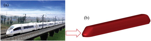
The CRH3 HST, which is a widely operated train in China, was taken as the research object. Figure 1 shows the external shape of the CRH3. The geometric model of the train is composed of the leading, middle and tail carriages. The windows, bogies and wheelsets have been omitted. The length (L), height (H) and width (W) of the train model are 76, 3.89 and 3.265 m, respectively. The cross-sectional area A_train is approximately 11.6 m². Although the train model is simplified, the train body, including the lengths of the tips and carriage, reproduces the key geometric features of its prototype. Such features have a vital influence on the train’s aerodynamics.

Figure 1. Comparison between the (a) full-scale CRH3 train and (b) numerical geometric model (mentioned in line 87).

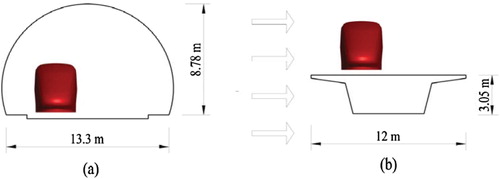
The tunnel has a width (W_t) and height (H_t) of approximately 13.3 and 8.78 m, respectively, with a cross-sectional area A_tunnel of 100 m². The blockage ratio β is approximately 11.6% (Figure 2(a)). The bridge has a width (W_v) and height (H_v) of approximately 12 and 3.05 m, respectively (Figure 2(b)). The train is located on a double line ballastless track configuration. The spacing (centreline distance) between two tracks is 5.0 m. These dimensions are specified for HSRs of 350 km/h in Code TB10621-2014. Certain details, such as track plate and rail, are omitted for efficient calculation. The comparison outcome of the corresponding model test results show that the omission is reliable (Deng, Yang, Lei, Zhu, & Zhang, 2019; Deng, Yang, Yin, & Zhang, 2019; Deng, Yang, & Zhang, 2019; Yang, Deng, Lei, Zhu, & Zhang, 2019).

Figure 2. Configuration of (a) tunnel and (b) bridge (front view) (mentioned in line 94).

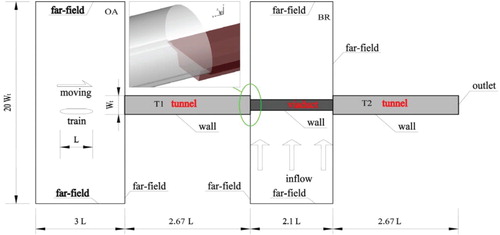
The model consists of the following regions: (1) an open-air (OA), (2) Tunnel 1 (T1), (3) bridge region (BR) and (4) Tunnel 2 (T2) (Figure 3). The configuration is based on the real scenario features of a Chinese HSR prototype, which is under construction. In the HSR prototype, the bridge, which is connected directly with two tunnels with lengths more than 7.6 and 8.5 km, respectively, has a length of approximately 159 m (2.1 L). If the model is reproduced strictly in accordance with the tunnel length of the engineering prototype, then the number of cells will be large to ensure efficient calculation or the cells will be particularly rough, thereby leading to unacceptable results. Therefore, the model adopted in this calculation decreases the lengths of the two tunnels. The model length of two tunnels is equal to 2.67 L. Although the length of the tunnel models is far less than that of the real-life prototypes, the 1D characteristics of the pressure distribution in the tunnel have been confirmed previously by numerous investigations. The pressure properties of an HST running in a long tunnel are related mainly to the aerodynamic drag effect, passenger discomfort and micro-pressure wave and only related slightly to HST running safety because of its balance pressure characteristics in a tunnel (Chen et al., 2017; Niu, Zhou, Liang, Liu, & Liu, 2017).

Figure 3. Schematic of computational domain and boundary condition (top view) (mentioned in line 101).

2.2. Computational domain and boundary conditions

Figure 3 presents a schematic of the computational domain and boundary condition. In region OA, the initial distance between the train nose tip and the inlet of T1 is 1.18 L. The length of region OA is 3 L. The boundary conditions of the ground, vehicle, tunnel and bridge surfaces are set as no-slip walls. The pressure-outlet condition is used at the T2 outlet. The OA and BR boundaries are applied through the pressure-far-field condition.

2.3. Meshing strategy

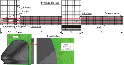
Using structural hexahedral grids, the entire computational zone is divided into three regions, namely, Regions 1, 2 and 3 (Figure 4). Regions 1 and 2 constitute the dynamic zone and Region 3 is a static one. The longitudinal dimensions of Region 1 grids are less than those of Region 2. The radial grid dimensions of Region 3 are enlarged gradually. The forward movement of the train is realized by layering the dynamic mesh method (Chu, Chien, Wang, & Wu, 2014; Deng, Yang, Lei, et al., 2019; Yang et al., 2019; Yang, Deng, Lei, Zhang, & Yin, 2018). V represents the HST speed and the flow field data for the two regions are passed by creating interface pairs. The entire model has approximately 4.5 million grids.

Figure 4. Schematic of the mesh model (side view) (mentioned in line 120).

2.4. Solution algorithm

Calculations are conducted using ANSYS-FLUENT CFD software. The finite volume method is used to solve the fluid governing equations. The discretised equations are solved through a semi-implicit method (Ferziger & Peric, 2002). The time step size is 1 × 10⁻³ s.

The flow field around the train presents significant dynamic response and turbulence characteristics when a train is passing the tunnel–bridge junction at high speed (Wang, Wu, Yang, Peng, & Qian, 2018; Chen, Liu, Yan, Yu, Guo, & Wang, 2019; Tao, Yang, Qian, Wu, & Wang, 2019). This flow field is suitable for assuming an incompressible Newtonian fluid for the Reynolds number greater than 10⁶ and Mach number less than 0.3. In the simulation of a high Reynolds number flow field, various approaches, such as LES and DES, exhibit significant advantages in terms of accuracy in reflecting a detailed change in the flow structure. However, the computational efficiency lessens with the high requirements in terms of mesh and time-step size (Niu et al., 2017). The RANS method (e.g. standard and RNG k–ε models) can address the accuracy demand of the engineering application and has high-computational efficiency in adapting to grid and time step (Choi & Kim, 2014; Chu et al., 2014; Niu et al., 2017; Yang et al., 2018). Thus, such a method is adopted in the present work to simulate the flow field when an HST is passing through the tunnel and bridge junction. The governing equations are as follows. (1) $\begin{array}{rl}& \frac{\mathrm{\partial }\rho }{\mathrm{\partial }t}+\frac{\mathrm{\partial }}{\mathrm{\partial }{x}_i}(\rho u_i)=0,\end{array}$(1) (2) $\begin{array}{rl}& \frac{\mathrm{\partial }}{\mathrm{\partial }t}(\rho u_i)+\frac{\mathrm{\partial }}{\mathrm{\partial }{x}_j}(\rho u_i{u}_j)\\ & =-\frac{\mathrm{\partial }p}{\mathrm{\partial }{x}_i}+\rho g{\delta }_{i3}+\frac{\mathrm{\partial }}{\mathrm{\partial }{x}_j}\left[\mu \left(\frac{\mathrm{\partial }{u}_i}{\mathrm{\partial }{x}_j}+\frac{\mathrm{\partial }{u}_j}{\mathrm{\partial }{x}_i}\right)-\frac{2}{3}{\delta }_{ij}\frac{\mathrm{\partial }{u}_l}{\mathrm{\partial }{x}_l}\right]\\ & +\frac{\mathrm{\partial }}{\mathrm{\partial }{x}_j}(-\rho \overline{{u^{\mathrm{\prime }}}_i{u^{\mathrm{\prime }}}_j})\end{array}$(2) where ρ represents the air density, p represents the pressure, u and u′ are the average and pulse speeds, respectively, μ represents the dynamic viscosity of the air, i and j represent the directions, g represents the gravitational acceleration and δ represents the Kronecker delta. The variable $-\rho \overline{{u^{\mathrm{\prime }}}_i{u^{\mathrm{\prime }}}_j}$ is related to the average speed gradients based on the Boussinesq equation and is calculated as follows: (3) $-\rho \overline{{u^{\mathrm{\prime }}}_i{u^{\mathrm{\prime }}}_j}={\mu }_t\left(\frac{\mathrm{\partial }{u}_i}{\mathrm{\partial }{x}_j}+\frac{\mathrm{\partial }{u}_j}{\mathrm{\partial }{x}_i}\right)-\frac{2}{3}\left(\rho k+{\mu }_t\frac{\mathrm{\partial }{u}_k}{\mathrm{\partial }{x}_k}\right){\delta }_{ij},$(3) where k represents the turbulent kinetic energy and ${\mu }_t$ represents the turbulent viscosity.

2.5. Case setting

Figure 5 presents a schematic of the composition of the wind velocity and HST speed vectors, where w represents the wind velocity relative to the ground, V represents the HST running speed, U represents the wind velocity relative to the HST, β represents the wind angle relative to the ground and α represents the wind angle relative to the HST.

Figure 5. Velocity triangles for a moving train simulation (mentioned in line 149).

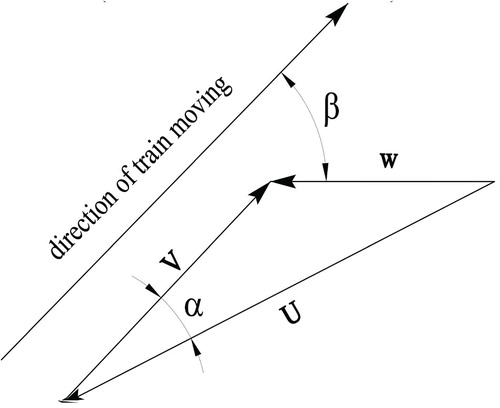
Table 1 illustrates the details of the wind and HST speeds used in the simulations, in which three independent parameters, namely, wind angle β (case C1s), wind velocity w (case C2s) and HST speed V (case C3s), are calculated. The three parameters are analyzed for two reasons. First, the aerodynamic coefficient characteristics in different wind environments and the train’s running condition are helpful for comprehending the aerodynamic response mechanism of an HST running in those scenarios. Second, such characteristics are necessary to acquire the safe domain of an HST running in the scenario in the future.

Table 1. Parameter settings used in calculation cases.

Case	β (°)	w (m.s^−1)	V (km.h^−1)
C1	30(C1A), 90(C1B), 150(C1C)	25	250
C2	90	0(C2A), 15(C2B), 20(C2C), 30(C2D)	250
C3	90	25	200(C3A), 300(C3B), 350(C3C)

2.6. Calculation of aerodynamic coefficients

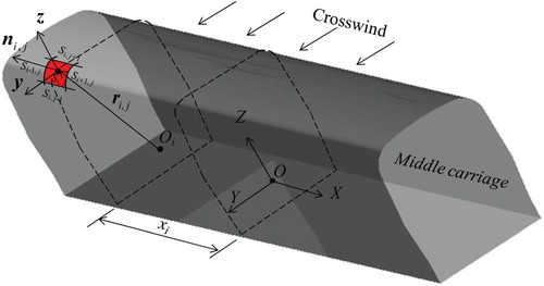
The five aerodynamic load indices related closely to train running safety are side force $F_{side}$, lift force $F_{lift}$, rolling moment $M_x$, yawing moment $M_z$ and pitching moment $M_y$ (Cai & Chen, 2004). Figure 6 shows the calculation schematic (take the middle carriage as an example). Eq. (4(4) $\begin{array}{rl}{F}_{side}& =\sum _{i=1}^n\left(\sum _{j=1}^k(p_{i,j}\cdot S_{i,j}\cdot ({\mathit{n}}_{i,j}\cdot \mathit{y}))\right)\\ F_{lift}& =\sum _{i=1}^n\left(\sum _{j=1}^k(p_{i,j}\cdot S_{i,j}\cdot ({\mathit{n}}_{i,j}\cdot \mathit{z}))\right)\\ M_x& =\sum _{i=1}^n\left(\sum _{j=1}^k(p_{i,j}\cdot S_{i,j}\cdot ({\mathit{r}}_{i,j}\times {\mathit{n}}_{i,j}))\right)\\ M_z& =\sum _{i=1}^n\left(\sum _{j=1}^k(p_{i,j}\cdot S_{i,j}\cdot ({\mathit{n}}_{i,j}\cdot \mathit{y})\cdot x_i)\right)\\ M_y& =\sum _{i=1}^n\left(\sum _{j=1}^k(p_{i,j}\cdot S_{i,j}\cdot ({\mathit{n}}_{i,j}\cdot \mathit{z})\cdot x_i)\right),\end{array}$(4) ) shows the calculation formula. In this formula, the center of the moment is the barycentre of the carriage body. (4) $\begin{array}{rl}{F}_{side}& =\sum _{i=1}^n\left(\sum _{j=1}^k(p_{i,j}\cdot S_{i,j}\cdot ({\mathit{n}}_{i,j}\cdot \mathit{y}))\right)\\ F_{lift}& =\sum _{i=1}^n\left(\sum _{j=1}^k(p_{i,j}\cdot S_{i,j}\cdot ({\mathit{n}}_{i,j}\cdot \mathit{z}))\right)\\ M_x& =\sum _{i=1}^n\left(\sum _{j=1}^k(p_{i,j}\cdot S_{i,j}\cdot ({\mathit{r}}_{i,j}\times {\mathit{n}}_{i,j}))\right)\\ M_z& =\sum _{i=1}^n\left(\sum _{j=1}^k(p_{i,j}\cdot S_{i,j}\cdot ({\mathit{n}}_{i,j}\cdot \mathit{y})\cdot x_i)\right)\\ M_y& =\sum _{i=1}^n\left(\sum _{j=1}^k(p_{i,j}\cdot S_{i,j}\cdot ({\mathit{n}}_{i,j}\cdot \mathit{z})\cdot x_i)\right),\end{array}$(4) where k and n are the number of segments along the circumferential and longitudinal directions, respectively, $p_{i,j}$ and $S_{i,j}$ are the mean pressure and area of the surface (ith, jth), respectively, ${\mathit{n}}_{i,j}$ is the unit normal vector of the surface (ith, jth). $\mathit{y}$ and $\mathit{z}$ are the unit vectors along the y and z directions, respectively, ${\mathit{r}}_{i,j}$ represents the moment arm vector on the ith cross-section and $x_i$ represents the longitudinal distance from the center of the surface (ith, jth) to the barycentre.

Figure 6. Calculation schematic of aerodynamic loads (mentioned in line 161).

The corresponding aerodynamic coefficients, $C_P$, $C_S$, $C_L$, $C_{RM}$, $C_{YM}$ and $C_{PM}$ are defined as follows: (5) $\begin{array}{rl}{C}_P& =(P-P_{\mathrm{\infty }})/0.5\rho U^2\\ C_S& =F_{side}/(0.5\rho U^2{A}_{side})\\ C_L& =F_{lift}/(0.5\rho U^2{A}_{side})\\ C_{RM}& =M_x/(0.5\rho U^2{A}_{side}{h}_{train})\\ C_{YM}& =M_z/(0.5\rho U^2{A}_{side}{h}_{train})\\ C_{PM}& =M_y/(0.5\rho U^2{A}_{side}{h}_{train}),\end{array}$(5) where $A_{side}$ is the area of the side face for a single carriage and $h_{train}$ refers to the characteristic height of the carriage.

3. Verification

3.1. Verification of mesh independence

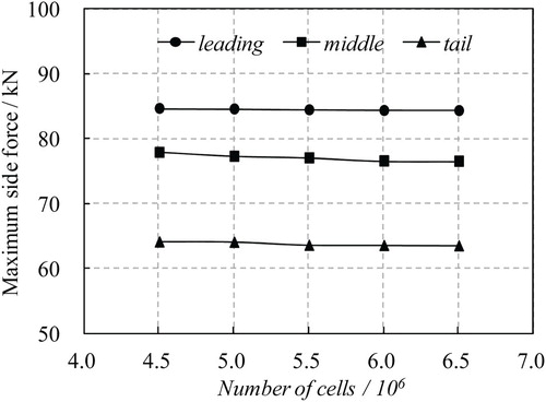
In this section, the mesh independence of the present model will be checked from two aspects, that is, the number of boundary layers and the mesh longitudinal resolution. The target indicator is the maximum $F_{side}$ of each carriage while a HST runs on flat ground under a crosswind. The calculation results of the four models with different numbers of boundary layers are compared (Figure 7). In each case, h₀, V, w and β remain constant. The figure shows that the target indicators tend to stabilize when the number of layers increases to eight. Figure 8 shows the comparison of target indicators for five models with different longitudinal mesh resolutions. The number of boundary layers for each model remains at eight. The figure shows that the target indicators of each model remain unchanged.

Figure 7. Maximum side force of three carriages under conditions of different boundary layer densities (V = 250 km/h, w = 25 m/s and β = 90°) (mentioned in line 179).

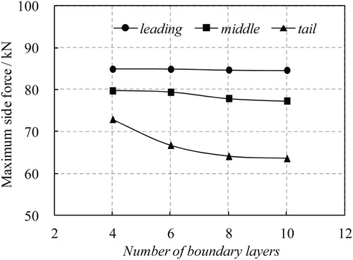
Figure 8. Maximum side force of three carriages under conditions of different cell numbers (V = 250 km/h, w = 25 m/s and β = 90°) (mentioned in line 180).

3.2. Verification of results

The results are compared with the field measurement data from Sui-Yu HSR to ensure reliability of the numerical method adopted in the present study. Two important field measurements on the same tunnel of that railway were reported by Wan and Wu (2006) and Han and Tian (2007). The test tunnel has a length of 1320 m and its cross-sectional area is 60 m² paved with a ballastless track. The train (CRH3) running speed is approximately 200 km/h. The numerical model used for validation in this section is reestablished to match the field test scenario. The measuring points for tunnel pressure wave are arranged in the tunnel at 223 m from the entrance, 1 m above the rail surface and 1 m from the tunnel surface (Wan & Wu, 2006). The measuring point of the train is located on the side window outside the driver’s cab (Han & Tian, 2007). The comparison of the time history of pressure between the test and this numerical simulation are shown in Figure 9. The figure shows that the algorithm adopted in this simulation can provide a good characterization on the unsteady effect during the tunnel entry of a train from open-air, particularly the transient response of pressure around the train, which is exactly the study focus.

Figure 9. Comparisons of time history of pressure between the test and this numerical simulation, (a) tunnel pressure wave data from Wan et al. [53]; (b) train pressure fluctuation data from Han et al. [54] (V = 200 km/h) (mentioned in line 193).

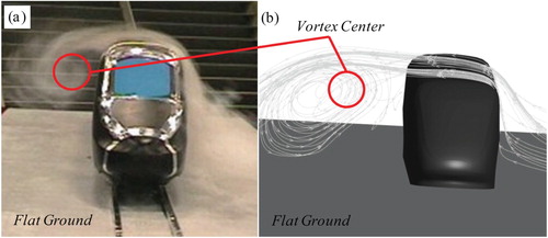
Figure 10 shows the comparison between the 3D flow around the train under crosswind action obtained through numerical simulation in the present study and the corresponding wind tunnel test results from Cheli, Ripamonti, Rocchi, and Tomasini (2010). Experimental analyzes have been performed on a 1: 10 scale model of the leading carriage of the EMUV 250 train in the Politecnico di Milano wind tunnel. The train model is paced on the flat ground. Train speed (V) is 0 km/h, the Reynolds number is 1.2 × 10⁶, and the wind angle (β) is 90°. In the numerical simulation, all the conditions are consistent with the experiment except the difference of train model. The flow field structures of the two studies are the same.

Figure 10. Comparison of (a) visual flow by wind tunnel test and (b) numerical simulation flow (mentioned in line 196).

4. Results and analysis

4.1. Flow field

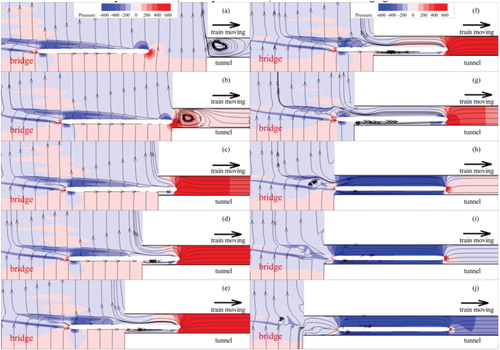
Figure 11 shows the evolution snapshots of the flow structure and pressure distribution around the train on a plane of 1.55 m above the rail top (TOR; approximately the height of the carriage’s gravity center) when a train moves from a tunnel into bridges under crosswind for case C2B (e.g. V = 250 km/h, w = 15 m/s and β = 90°).

Figure 11. Structure evolution of pressure and flow in the spanwise direction (1.55 m above the TOR) as train runs from tunnel 1 to bridge with crosswind (V = 250 km/h, w = 15 m/s and β = 90°) (mentioned in line 205).

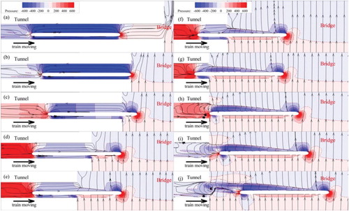
When the HST runs completely in the tunnel (Figure 11(a)), the flow field structure shows fundamental symmetry in the span-wise direction. The streamline originates from the train nose, revolves around the train and reaches the train’s tail. The pressure generally remains unchanged between the windward and leeward flank regardless of whether it increases due to the compression wavefronts or decreases due to the expansion wavefronts. Various characteristics, such as the flow field structures and pressure distribution on the lateral flanks of the train, continue until the nose tip arrives at the T1 outlet (Figure 11(b)).

When several segments of a train come out from the tunnel into the bridge environment under the crosswind condition (Figure 11(c–g)), striking flow asymmetry appears on the two sides of the carriage segment on the bridge. The wind is blocked by the carriage in the windward flanks and the surface pressure on the corresponding segment of carriage increases. Meanwhile, a vortex is generated in the train leeward flank, which originates from the rear of the leading carriage rather than the nose tip (Figure 11(c and d)), indicating reasonable agreement with a previously reported investigation (Khier, Breuer, & Durst, 2000). The surface pressure of the train in the leeward side will decrease because of the vortex effect. The differences in the flow structure is not significant regardless of just the tip of the train’s tail leaving the tunnel (Figure 11(h)), or if the whole train moves far from the tunnel (Figure 11(i and j)), except for the wake slipstream structure.

The rapid transformation of infrastructure scenario causes the transient variation in the aerodynamic properties on the train body when running at the junction location of the tunnel and bridge. Figures 12–14 illustrate certain cross-sectional diagrams of the flow and pressure in the tunnel exit vicinity the moment the longitudinal middle of each carriage reaches the exit of T1. This undertaking is initiated to observe the effects of the transformation of infrastructure scenarios on the flow field structure and pressure distribution on the vertical surface of the train. The positive pressure region is noted with a red line and the negative pressure is indicated with a blue one. Meanwhile, the static pressure on the lateral surface of the whole HST is provided at the corresponding instances.

Figure 12. Pressure distribution around the entrance when the middle of the leading carriage reaches the tunnel 1 exit (V = 250 km/h, w = 15 m/s, β = 90° and the same instant as in Figure 12(c)) (mentioned in line 224).

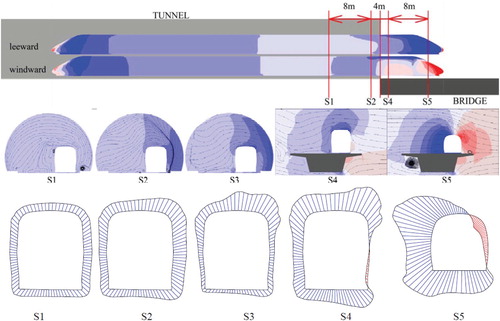
Figure 13. Pressure distribution around the entrance when the middle of the second carriage reaches the tunnel 1 exit (V = 250 km/h, w = 15 m/s, β = 90° and the same instant as in Figure 12(e)) (mentioned in line 234).

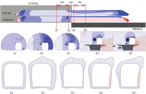
Figure 14. Pressure distribution around the entrance when the middle of the tail carriage reaches the tunnel 1 exit (V = 250 km/h, w = 15 m/s, β = 90° and the same instant as in Figure 12(g)) (mentioned in line 224).

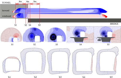
The aforementioned figures show a sharp variation in the windward side position is generated at the tunnel exit for the static pressure on the lateral surface. For the train segment in the tunnel, the pressure is influenced by the pressure waves and shows symmetry, especially for the section deep inside the tunnel (e.g. S1). A tiny vortex is observed on the top flank when the middle carriage reached the T1 exit, thereby causing the low-pressure region on the middle top flank (S2 in Figure 13). For the segment in the bridge, the surface pressure of the train is influenced considerably by the crosswind. The static pressure on the flank is positive in the windward side but negative in the leeward side because of the coupling effect of separation flow and vortex. Separation flow influences the leading carriage (Figure 12). The coupling effect of separation flow and vortex influences the middle and tail carriages (Figures 13 and 14). In the leeward side, only one vortex is observed at the upper corner for the middle carriage (Figure 13). By contrast, two vortices are located at the upper and bottom corners for the tail carriage (Figure 14). These findings agree with the results of a previous investigation (Khier et al., 2000). The side force and rolling moment are likely generated for different pressures on the lateral flanks. The yaw moment will be excited for different pressures and flow structures of different carriages.

For the train segment in the bridge, the variation in pressure distribution is generated in the lateral and vertical flanks. The pressure on the top flank is negative due to separation flow, especially at the windward corner. Such flow at the windward corner is greatly strong that maximum negative pressure exists at the windward top in the cross-sectional plane (e.g. S4 for each carriage). Separation flow that represents the low-pressure regions is also observed on the bottom flank, especially at the windward corner for the leading carriage (S4 in Figure 12) and leeward corner for the tail carriage (S4 in Figure 14).

Pressure imbalance is related to the relative distance with respect to the tunnel exit. For instance, the surface static pressure in Figure 13 shares a similar distribution for sections S1 and S2 even though the two sections are separated by approximately 8 m. By contrast, the surface static pressure shares a significantly different distribution for S2 and S3 even though the two sections are separated by only 2 m. Such a phenomenon can also be obtained for sections S3, S4 and S5 in Figure 13. Consequently, the sudden variation in pressure distribution around a train is generated within a limited range near the tunnel exit, indicating a transient aerodynamic shock for an HST. Thus, the reaction time of pressure variation from S2 to S4 does not exceed 0.1 s for the train speed of 250 km/h. However, the duration time of response of the vehicle body caused by this change is about 1.5 s, and the corresponding amplitude of lateral displacement is at most 150 mm (Deng, Yang, Lei, et al., 2019).

The sudden variation in the flow structure and pressure distribution follows immediately when the train runs from the bridge under crosswind condition into the tunnel (Figure 15). The variation in pressure distribution near the HST is observed from the imbalanced state in a bridge to the balanced state in the tunnel, which is in contrast with the variation process of a train exiting from T1. The imbalanced pressure around the train inevitably leads to unsteady aerodynamic loads on the train body. Such loads are regarded as a potential hazard and a necessary parameter of safety assessment for a running train.

Figure 15. Structure evolution of pressure and flow in the spanwise direction (1.55 m above the TOR) as the train runs from bridge into tunnel 2 (V = 250 km/h, w = 15 m/s and β = 90°) (mentioned in line 259).

4.2. Aerodynamic loads

Figure 16 illustrates the time histories of transient aerodynamic loads for case C2B (e.g. V = 250 km/h, w = 15 m/s and β = 90°) in the left. The time histories of the aerodynamic forces and moments for non-crosswind (case C2A) are illustrated on the right for comparison. The initial position of different aerodynamic loads at the instant the train reaches the tunnel and bridge junction differs. The whole time histories are provided for full comprehension of the transient response of five aerodynamic loads. A specific reference time is followed. For example, t = 0 s corresponds to the time that the leading tip reaches the entrance of T1 from open air; t = 2.88, 3.24 and 3.60 s correspond to the instant that the front of the leading, middle and tail carriages reaches the T1 exit, respectively; and t = 5.17, 5.53 and 5.89 s correspond to the instant the front of the leading, middle and tail carriages reaches the T2 entrance, respectively. The duration of each carriage exiting or entering the tunnel entrance is 0.36 s when the train speed is 250 km/h.

Figure 16. Evolution of aerodynamic forces and moments with respect to time during a moving train in the infrastructure scenarios: from tunnel to bridge (crosswind) and then enter tunnel again (V = 250 km/h, w = 15 m/s (left) and 0 m/s (right), β = 90°) (mentioned in line 265).

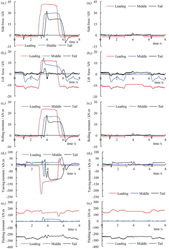
The magnitude of aerodynamic forces and moments with crosswind anywhere is trivial regardless of whether the whole train runs in T1 or T2 but becomes substantial in the bridge. The side force value is approximately −2.4 kN for the leading carriage but increases to −0.3 kN for the middle and tail carriages when the train runs in tunnels. The steady values of side force are approximately 41.6, 29.2 and 20.4 kN for the leading, middle and tail carriages in the bridge, respectively. The side force points to the near-wall side when the train inside the tunnel or the leeward side runs on the bridge (Figure 16(a)). The steady values of the lift force are approximately −12.6, −4.8 and 1.9 kN and 11.4, 7.8 and 0.3 kN for the leading, middle and tail carriages in the tunnel and bridge, respectively. The lift force direction points downwards in the tunnel but upwards in the bridge (Figure 16(b)). The variation law of rolling moment is similar to that of the side force (Figure 16(c)). The steady values of yaw moment are approximately −7.9, 0.2 and 17.4 kN/m and −134, 17.3 and −118.3 kN/m for the leading, middle and tail carriages in the tunnel and bridge, respectively. The positive direction of the yaw moment turns clockwise, thereby indicating that the front of the leading carriage turns to the windward (i.e. near-wall) side whether it runs inside the tunnel or on the bridge; the front-end of the middle car turns to the far-wall (i.e. leeward) side whether it runs in the tunnel or on the bridge; the front of the tail carriage turns to the near-wall side when it runs in the tunnel but to the leeward side when it runs on the bridge (Figure 16(d)). The steady values of pitch moment are approximately 169, 0.2 and −248 kN/m and 140, 32 and −236.5 kN/m for the leading, middle and tail carriages in the tunnel and bridge, respectively. The front of the leading and middle carriages turns upwards, whereas that of the tail carriage turns downwards. Such a phenomenon indicates that the crosswind slightly influences the magnitude evolution of pitch moment but does not influence the pitch moment evolution of direction (Figure 16(e)).

The oscillation of a vehicle’s aerodynamic coefficients is considerable when it is subjected to the gusty wind (Tsubokura et al., 2010). A sharp shock in the aerodynamic forces and moments is generated at the moment when the train runs at the tunnel and bridge junction, regardless of whether from T1 to the bridge or from the bridge to T2. The steady values of the aerodynamic loads are non-synchronous in the evolution of different carriages after it reaches the junction location. The evolution of the aerodynamic forces and moments is followed based on the maximum and steady values. For the side force, the steady value of the leading and middle carriages reaches as soon as the whole body of carriage has arrived in a crosswind. The side force increases monotonically with time (Tsubokura et al., 2010). Although the side force of the tail carriage peaks at t = 3.93 s, this maximum is maintained until t = 4.34 s when the side force is steady. Such a phenomenon of the tail carriage is visible in the investigation (Volpe et al., 2014). For the lift force, the value of the leading carriage peaks at t = 2.93 s and reaches its steady equivalent at t = 2.98 s. The value of the middle and tail carriages reaches its maximum at t = 3.19 s and t = 3.31 s, respectively. The corresponding carriages have yet reached the entrance at these moments. The steady values of the leading and middle carriages reach t = 3.12 and 3.42 s, respectively. The lift force of the tail carriage continues to vary up and down around zero, and it has been unsteady. The yaw moment of the leading carriage first overshoots in the initial stage of rushing; it reaches its maximum at t = 2.77 s and then decreases monotonically after t = 2.97 s. By contrast, the yaw moment of the middle carriage first reaches 32.4 kN/m at t = 2.91 s, decreases to its maximum of −91.77 kN/m at t = 3.14 s and finally increases to its steady value of 17.03 kN/m at t = 3.59 s. The yaw moment of the tail carriage shows two overshoots (at t = 3.22 and 3.44 s for the positive and negative values) before establishment. The pitch moment for each carriage first overshoots undershoots and reaches establishment.

Different aerodynamic loads show time-resolved discrepancy as a train runs in ISTBT. The maximum side force of the leading and middle carriages is later than the instant that the whole body is entirely on the bridge in the crosswind because of the phase delay of the flow (Tsubokura et al., 2010; Volpe et al., 2014). However, other aerodynamic parameters are earlier based on this unsteady simulation. With the yaw moment as an example, the maximum value is generated when the geometric center of each carriage reaches the junction location of the tunnel and bridge. This discrepancy may be because of the difference in the crosswind condition between the numerical simulation and the wind tunnel investigation. In the wind tunnel investigation, gust is applied to the vehicle whole body. By contrast, crosswind is gradually applied to the train body in the real-life operation as the train moves from the tunnel in the longitudinal direction.

The time-resolved effects of scenario transformation influence the time synchronization and magnitude of transient aerodynamic loads. The comparison between the maximum and the steady values of five aerodynamic loads is provided in Table 2 to fully assess the transient response. The sharp shock induced by crosswind when a train runs in the ISTBT exerts a more serious influence than that from transient crosswinds (Tsubokura et al., 2010; Volpe et al., 2014). In particular, the yaw moment exceeds the corresponding steady values up to 71%, 628% and −17% for the leading, middle and tail carriages, respectively.

Table 2. Comparison between the maxima and steady values of aerodynamic response.

Value		Max.	Ste.	[(Max.−Ste.) / Ste.] × 100%
Leading	$F_{side}(kN)$	41.6	41.3	0.7%
	$F_{lift}(kN)$	12.2	11.4	7%
	$M_z(kN.m)$	−229	−134	71%
	$M_y(kN.m)$	172.2	132.1	30%
Middle	$F_{side}(kN)$	29.2	29.1	0.3%
	$F_{lift}(kN)$	14.2	8.1	75%
	$M_z(kN.m)$	−91.3	17.3	−628%
	$M_y(kN.m)$	58.4	32.5	80%
Tail	$F_{side}(kN)$	31.7	20.4	55%
	$F_{lift}(kN)$	4.7	0.7	571%
	$M_z(kN.m)$	−98.3	−118.3	−17%
	$M_y(kN.m)$	−264.8	−234.4	13%

The transient aerodynamic response of the tail carriage is noteworthy and does not reach a steady state. The value of the aerodynamic force usually shakes around the so-called steady value. The possible reason may be attributed to the unsteady wake structure of the HST, which witnesses a strong span-wise oscillation (Bell, Burton, Thompson, Herbst, & Sheridan, 2016a, 2016b, 2017a, 2017b; Chometon et al., 2005).

Relative to the case without crosswind, the aerodynamic forces and moments without crosswind exhibit a trivial variation due to the boundary asymmetry regardless if the train runs in T1, bridge, T2, or at the junction location (Figure 16(a₂–e₂)).

4.3. Analysis of influence factors

4.3.1. Wind speed

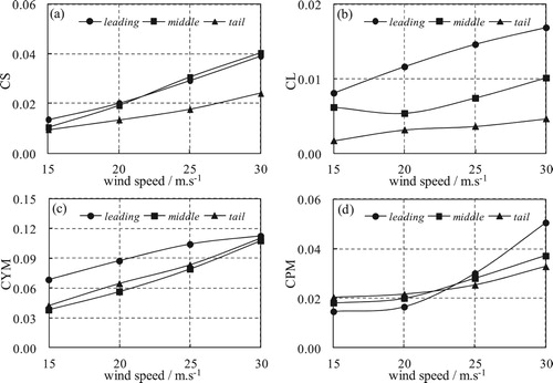
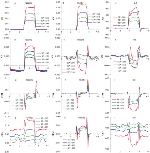
Figure 17 shows a comparison of the time histories of the four aerodynamic coefficients (i.e. side force C_S, lift force C_L, yawing moment C_YM and pitching moment C_PM) of a moving train in the ISTBT for different crosswind speeds. The aerodynamic coefficients are significantly influenced by wind speed. All coefficients increase with the increase in wind speed, except for the lift coefficients of the middle and tail carriages (Figure 17(e and f)). The steady value of the lift coefficient of the middle carriage is positive for 15 m/s, thereby indicating that the lift force direction is upward. By contrast, the steady value is negative when the wind speed is equal to or larger than 20 m/s, thereby showing that the lift force direction is downward. Although the downward direction of the lift force is generally beneficial to the running stability of a train, the negative steady value of lift is likely to reduce the running safety because of the large gap between the steady and the maximum values. At the precise moment when a HST runs from the bridge into T2, the lift force direction converts rapidly from downward to upward. The lift coefficient of the tail carriage does not monotonically increase with the increase in wind speed. The steady value for 25 m/s wind is larger than those for 15, 20 and 30 m/s wind. Such a phenomenon may be attributed to the unsteady wake structure of the HST. This issue should be further examined in the future. Figure 18 shows the peak-to-peak value of the four aerodynamic coefficients with respect to wind velocity during a train moving in this scenario for ease of comprehension of the transient response of aerodynamic coefficients.

Figure 17. Time history comparison of aerodynamic coefficients during a moving train in the ISTBT for different crosswind speeds (V = 250 km/h and β = 90°) (mentioned in line 338).

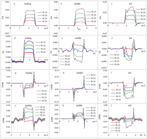
Figure 18. P-P value of aerodynamic coefficients with respect to wind speed during a moving train in the infrastructure scenarios: from tunnel to bridge (crosswind) and then into tunnel again (V = 250 km/h and β = 90°) (mentioned in line 350).

4.3.2. Train speed

Figure 19 shows the comparison of the time history of the four aerodynamic load coefficients during a moving train in the ISTBT for different train speeds. The time in Figure 19 is normalized as the reference time τ based on the time history of 250 km/h for ease of comparison. Thus, the following relations are expected: (6) $\tau =t_{250}\frac{T_s}{250},$(6) where τ is the reference time, t₂₅₀ is the time history of train running in 250 km/h and T_s is the normalized train speed.

Figure 19. Time history comparison of aerodynamic coefficients during a moving train in the ISTBT for different train speeds (w = 25 m/s and β = 90°) (mentioned in line 354).

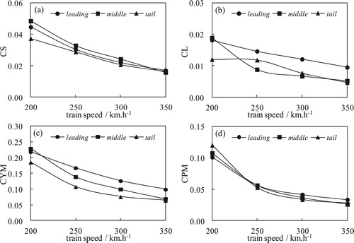
Relative to the crosswind speed, the values of aerodynamic coefficients, regardless of the maximum value or the steady one, decrease with the increase in train speed, except for the lift coefficient of the tail carriage (Figure 19(f)). The lift steady value of the tail carriage for 200 km/h train speed is approximately equal to that for 300 km/h but lower than that for 250 km/h. The wake slipstream oscillation of the train may also be a possible reason. Figure 20 shows the peak-to-peak value of the four aerodynamic coefficients with respect to train speed.

Figure 20. P-P value of aerodynamic coefficients with respect to train speed during a moving train in the infrastructure scenarios: from tunnel to bridge (crosswind) and then into tunnel again (w = 25 m/s and β = 90°) (mentioned in line 363).

4.3.3. Wind angle

The effect of the yaw angle on the aerodynamic coefficients is studied by comparing the results of three different wind angles, namely, 30°, 90° and 150°. The time history comparison and peak-to-peak value of the four aerodynamic coefficients with respect to wind angle are shown in Figures 21 and 22, respectively.

Figure 21. Time history comparison of aerodynamic coefficients during a moving train in the ISTBT for different wind angles (w = 25 m/s and V = 250 km/h) (mentioned in line 368).

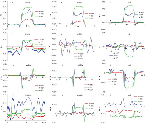
Figure 22. P-P value of aerodynamic coefficients with respect to wind angle during a moving train in the infrastructure scenarios: from tunnel to bridge (crosswind) and then into tunnel again (w = 25 m/s and V = 250 km/h) (mentioned in line 368).

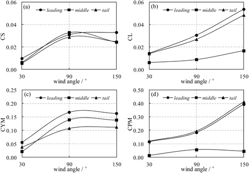
In general, the wind with a direction perpendicular to that of a moving train will likely exaggerate the steady value of the aerodynamic coefficients. Wind from the reverse direction may increase the transient variation in the aerodynamic coefficients, thereby indicating that the train will suffer from a transient aerodynamic response. Wind from the following direction can help reduce the crosswind influence for the steady and maximum values of the aerodynamic coefficients. With side force coefficients as an example, the wind angles β equal to 30°, 90° and 150° correspond to the wind from the reverse, perpendicular and following directions.

The side force coefficients of the case 90° (C1B) are larger than those of 30° and 150°. This phenomenon can be explained through the parallelogram law of velocity (Figure 5). The dynamic pressure of all crosswinds turns the static pressure on the train body for β = 90°, and thus, the side force is larger than the other two. For β = 30°, the direction of wind reverses that of a moving car and the yaw angle α decreases when other conditions remain the same. Accordingly, the absolute wind speed U is reduced. For β = 150°, the absolute wind speed U and α decrease simultaneously and thus, the side coefficients are lower than the others. Therefore, the wind whose direction follows that of a moving train is helpful in decreasing the side force of the train.

5. Conclusions

This study examined the evolution of the flow structure and aerodynamic force when a train runs through the ISTBT under a crosswind. The impacting mechanism of airflow on the train body, characteristics and relational parameters of the transient variation in the aerodynamic forces are also investigated. The following conclusions can be drawn:

1. The flow structure and pressure distribution around a train are symmetric when runs in a tunnel but asymmetric in a bridge. A sharp variation in the flow structure and pressure distribution is generated at the junction location of the tunnel and the bridge under a crosswind. Accordingly, a sudden variation is generated in all five aerodynamic coefficients.

2. The time-resolved characteristics of the five aerodynamic forces on the train body should be considered when assessing the safety risk of trains when they run under the coupling effects of crosswind and scenario transformation. The coupling effect between the crosswind environment and scenario transformation of running trains will likely influence the transient aerodynamic response in two aspects.

   1. First, not all aerodynamic coefficients reach their maximum value when the train is dipped entirely in the crosswind. The maximum side force of the leading and middle carriages is later than the instant the whole body is dipped entirely in bridge in the crosswind because of the phase delay of the flow field.

   2. Second, the differences between the maximum and the steady values of the five aerodynamic loads are much larger than those of road vehicle under gust wind, as already observed in the literature. The transient response of different coefficients varies significantly depending on the differences between the steady and the maximum values of the aerodynamic loads, such as the change ratio range from 0% to 628%.

3. The transient magnitude (peak-to-peak value) of the aerodynamic coefficients when an HST runs in the ISTBT under crosswind increases with the increase in wind speed but decreases with the increase in train speed when other conditions remain the same.

4. Wind angle has a remarkable influence on the transient response of a running train. The forward wind is helpful to lighten the transient aerodynamic response as the maxima and steady value of coefficients decrease significantly. The opposite wind will likely strengthen the transient aerodynamic response depending on the gap between the maxima and the steady values of the aerodynamic coefficients.

Given the lack of relevant field measurement and model testing, the results obtained in this investigation should be verified further. Thus, follow-up research should focus on safety coefficients obtained from wind–train–track–bridge dynamic coupled analytical system.

Acknowledgment

This work was supported by the National Natural Science Foundation of China (Grant Nos. 51978670 and U1534206) and the Fundamental Research Funds for the Central Universities of Central South University (Grant No. 2019zzts291). The authors are grateful for the supports awarded. In addition, the authors would like to thank Ms. Xinyang Li for her great support for this paper.

Disclosure statement

No potential conflict of interest was reported by the authors.

Additional information

Funding

This work was supported by the National Natural Science Foundation of China [grant numbers 51978670 and U1534206]; the Fundamental Research Funds for the Central Universities of Central South University [grant number 2019zzts291].

References

- Alonso-Estebanez, A., Del Coz Diaz, J. J., Alvarez Rabanal, F. P., & Pascual-Munoz, P. (2017). Numerical simulation of bus aerodynamics on several classes of bridges decks. Engineering Applications of Computational Fluid Mechanics, 11(1), 435–449. doi: 10.1080/19942060.2016.1201544
- Baker, C. J. (2010). The simulation of unsteady aerodynamic cross wind forces on trains. Journal of Wind Engineering and Industrial Aerodynamics, 98, 88–99. doi: 10.1016/j.jweia.2009.09.006
- Bell, J. R., Burton, D., Thompson, M. C., Herbst, A. H., & Sheridan, J. (2016a). Flow topology and unsteady features of the wake of a generic high-speed train. Journal of Fluids and Structures, 61, 168–183. doi: 10.1016/j.jfluidstructs.2015.11.009
- Bell, J. R., Burton, D., Thompson, M. C., Herbst, A. H., & Sheridan, J. (2016b). Dynamics of trailing vortices in the wake of a generic high-speed train. Journal of Fluids and Structures, 65, 238–256. doi: 10.1016/j.jfluidstructs.2016.06.003
- Bell, J. R., Burton, D., Thompson, M. C., Herbst, A. H., & Sheridan, J. (2017a). The effect of tail geometry on the slipstream and unsteady wake structure of high-speed trains. Experimental Thermal and Fluid Science, 83, 215–230. doi: 10.1016/j.expthermflusci.2017.01.014
- Bell, J. R., Burton, D., Thompson, M. C., Herbst, A. H., & Sheridan, J. (2017b). A wind-tunnel methodology for assessing the slipstream of high-speed trains. Journal of Wind Engineering and Industrial Aerodynamics, 166, 1–19. doi: 10.1016/j.jweia.2017.03.012
- Cai, C. S., & Chen, S. R. (2004). Framework of vehicle–bridge–wind dynamic analysis. Journal of Wind Engineering and Industrial Aerodynamics, 92, 579–607. doi: 10.1016/j.jweia.2004.03.007
- Cairns, R. S. (1994). Lateral aerodynamic characteristics of motor vehicles in transient crosswinds (Ph.D. Thesis). Cranfield University, UK.
- Cheli, F., Ripamonti, F., Rocchi, D., & Tomasini, G. (2010). Aerodynamic behaviour investigation of the new EMUV250 train to cross wind. Journal of Wind Engineering and Industrial Aerodynamics, 98, 189–201. doi: 10.1016/j.jweia.2009.10.015
- Chen, J. W., Gao, G. J., & Zhu, C. L. (2016). Detached-eddy simulation of flow around high-speed train on a bridge under cross winds. Journal of Central South University, 23, 2735–2746. doi: 10.1007/s11771-016-3335-2
- Chen, Z. W., Liu, T. H., Yan, C. G., Yu, M., Guo, Z. J., & Wang, T. T. (2019). Numerical simulation and comparison of the slipstreams of trains with different nose lengths under crosswind. Journal of Wind Engineering and Industrial Aerodynamics, 190, 256–272. doi: 10.1016/j.jweia.2019.05.005
- Chen, Z. W., Liu, T. H., Zhou, X. S., & Niu, J. Q. (2017). Impact of ambient wind on aerodynamic performance when two trains intersect inside a tunnel. Journal of Wind Engineering and Industrial Aerodynamics, 169, 139–155. doi: 10.1016/j.jweia.2017.07.018
- Chen, X. Y., Wang, B., Zhu, L. D., & Li, Y. L. (2018). Numerical study on surface distributed vortex-induced force on a flat-steel-box girder. Engineering Applications of Computational Fluid Mechanics, 12(1), 41–56. doi: 10.1080/19942060.2017.1337593
- Cheng, S. Y., Tsubokura, M., Nakashima, T., Okada, Y., & Nouzawa, T. (2012). Numerical quantification of aerodynamic damping on pitching of vehicle-inspired bluff body. Journal of Fluids and Structures, 30, 188–204. doi: 10.1016/j.jfluidstructs.2012.01.002
- Choi, J. K., & Kim, K. H. (2014). Effects of nose shape and tunnel cross-sectional area on aerodynamic drag of train traveling in tunnels. Tunnelling and Underground Space Technology, 41, 62–73. doi: 10.1016/j.tust.2013.11.012
- Chometon, F., Strzelecki, A., Ferrand, V., Dechipre, H., Dufour, P. C., Gohlke, M., & Herbert, V. (2005). Experimental study of unsteady wakes behind an oscillating car model. SAE Technical Paper No. 2005-01-0604.
- Chu, C. R., Chien, S. Y., Wang, C. Y., & Wu, T. R. (2014). Numerical simulation of two trains intersecting in a tunnel. Tunnelling and Underground Space Technology, 42, 161–174. doi: 10.1016/j.tust.2014.02.013
- Deng, L., Yan, W. C., & Nie, L. (2019). A simple corrosion fatigue design method for bridges considering the coupled corrosion-overloading effect. Engineering Structures, 178, 309–317. doi: 10.1016/j.engstruct.2018.10.028
- Deng, E., Yang, W. C., Lei, M. F., Zhu, Z. H., & Zhang, P. P. (2019). Aerodynamic loads and traffic safety of high-speed trains when passing through two windproof facilities under crosswind: A comparative study. Engineering Structures, 188, 320–339. doi: 10.1016/j.engstruct.2019.01.080
- Deng, E., Yang, W. C., Yin, R. S., & Zhang, P. P. (2019). Study on transient aerodynamic performance of high-speed trains when entering into tunnel under crosswinds. Journal of Hunan University (Natural Sciences), 46(9), 69–78 (in Chinese ).
- Deng, E., Yang, W. C., & Zhang, P. P. (2019). Impact effect of aerodynamic loads on high-speed trains when entering into tunnel under crosswinds. Journal of South China University of Technology (Natural Science Edition), 47(10), 130–138 (in Chinese ).
- Ferrand, V., & Grochal, B. (2012, July 8–12). Forces and flow structures on a simplified car model exposed to a transient crosswind. Proceedings of the ASME 2012 Fluids Engineering Summer Meeting, Rio Grande, Puerto Rico.
- Ferziger, J., & Peric, M. (2002). Computational method for fluid dynamics (3rd ed.). Berlin Heidelberg, Germany: Springer.
- Han, K., & Tian, H. Q. (2007). Research and application of testing technology of aerodynamics at train-tunnel entry on special passenger railway lines. Journal of Central South University (Science & Technology), 38(2), 326–332 (in Chinese).
- Hu, P., Li, Y. L., Huang, G. Q., Kang, R., & Liao, H. L. (2015). The appropriate shape of the boundary transition section for a mountain-gorge terrain model in a wind tunnel test. Wind and Structures, 20(1), 15–36. doi: 10.12989/was.2015.20.1.015
- Khier, W., Breuer, M., & Durst, F. (2000). Flow structure around trains under side wind conditions: A numerical study. Computers and Fluids, 29, 179–195. doi: 10.1016/S0045-7930(99)00008-0
- Li, Y., Hu, P., Cai, C. S., Zhang, M., & Qiang, S. (2013). Wind tunnel study of a sudden change of train wind loads due to the wind shielding effects of bridge towers and passing trains. Journal of Engineering Mechanics, 139(9), 1249–1259. doi: 10.1061/(ASCE)EM.1943-7889.0000559
- Li, Y., Hu, P., Xu, X., & Qiu, J. (2017). Wind characteristics at bridge site in a deep-cutting gorge by wind tunnel test. Journal of Wind Engineering and Industrial Aerodynamics, 160, 30–46. doi: 10.1016/j.jweia.2016.11.002
- Li, D. S., Ma, Z. F., Xu, Z. L., & Chen, H. L. (2011). Design and research of bridge-tunnel joint technology on Changsha-Kunming passenger dedicated line. Journal of Railway Engineering Society, 159(12), 69–79 (in Chinese).
- Liu, T. H., Chen, Z. W., Zhou, X. S., & Zhang, J. (2018). A CFD analysis of the aerodynamics of a high-speed train passing through a windbreak transition under crosswind. Engineering Applications of Computational Fluid Mechanics, 12(1), 137–151. doi: 10.1080/19942060.2017.1360211
- Niu, J. Q., Zhou, D., & Liang, X. F. (2018). Numerical investigation of the aerodynamic characteristics of high-speed trains of different lengths under crosswind with or without windbreaks. Engineering Applications of Computational Fluid Mechanics, 12(1), 195–215. doi: 10.1080/19942060.2017.1390786
- Niu, J. Q., Zhou, D., Liang, X. F., Liu, T. H., & Liu, S. (2017). Numerical study on the aerodynamic pressure of a metro train running between two adjacent platforms. Tunnelling and Underground Space Technology, 65, 187–199. doi: 10.1016/j.tust.2017.03.006
- Ryan, A., & Dominy, R. (2000). Wake surveys behind a passenger car subjected to a transient cross-wind gust. SAE Technical Paper No. 2000-01-0874.
- Shi, C. H., Lei, M. F., Peng, L. M., & Zhao, D. (2011). Influenced factors of static-dynamic character about tunnel-bridge structure. Journal of Central South University (Science and Technology), 42(4), 1085–1091 (in Chinese).
- Tao, Y., Yang, M. D., Qian, B. S., Wu, F., & Wang, T. T. (2019). Numerical and experimental study on ventilation panel models in a subway passenger compartment. Engineering, 5, 329–336. doi: 10.1016/j.eng.2018.12.007
- Tsubokura, M., Nakashima, T., Kitayama, M., Ikawa, Y., Doh, D., & Kobayashi, T. (2010). Large eddy simulation on the unsteady aerodynamic response of a road vehicle in transient crosswinds. International Journal of Heat and Fluid Flow, 31, 1075–1086. doi: 10.1016/j.ijheatfluidflow.2010.05.008
- Volpe, R., Ferrand, V., Da Silva, A., & Le Moyne, L. (2014). Forces and flow structures evolution on a car body in a sudden crosswind. Journal of Wind Engineering and Industrial Aerodynamics, 128, 114–125. doi: 10.1016/j.jweia.2014.03.006
- Wan, X. Y., & Wu, J. (2006). In-situ test and study on the aerodynamic effect of the rolling stock passing through tunnels with a speed of 200km/h. Modern Tunnelling Technology, 143(1), 43–48 (in Chinese).
- Wang, T. T., Wu, F., Yang, M. Z., Peng, J., & Qian, B. S. (2018). Reduction of pressure transients of high-speed train passing through a tunnel by cross-section increase. Journal of Wind Engineering and Industrial Aerodynamics, 183, 235–242. doi: 10.1016/j.jweia.2018.11.001
- Yang, W. C., Deng, E., Lei, M. F., Zhang, P. P., & Yin, R. S. (2018). Flow structure and aerodynamic behavior evolution during train entering tunnel with entrance in crosswind. Journal of Wind Engineering and Industrial Aerodynamics, 175, 229–243. doi: 10.1016/j.jweia.2018.01.018
- Yang, W. C., Deng, E., Lei, M. F., Zhu, Z. H., & Zhang, P. P. (2019). Transient aerodynamic performance of high-speed trains when passing through two windproof facilities under crosswinds: A comparative study. Engineering Structures, 188, 729–744. doi: 10.1016/j.engstruct.2019.03.070
- Zhu, Z. H., Gong, W., Wang, L. D., Bai, Y., Yu, Z. W., & Zhang, L. (2019). Efficient assessment of 3D train-track-bridge interaction combining multi-time-step method and moving track technique. Engineering Structures, 183, 290–302. doi: 10.1016/j.engstruct.2019.01.036
- Zhu, Z. H., Gong, W., Wang, L. D., Li, Q., Bai, Y., Yu, Z. W., & Harik, I. E. (2018). An efficient multi-time-step method for train-track-bridge interaction. Computers and Structures, 196, 36–48. doi: 10.1016/j.compstruc.2017.11.004