Numerical simulation and analysis of five-stage lifting pump by improved turbulence model and catastrophe theory

Abstract

How to theoretically describe the process of turbulence formation emains an unsolved problem. A new method is presented in this paper for quantitatively researching the turbulence phase transition based on a dimensionless method and catastrophe theory. Then, the formula of energy spectrum density E_k, with the wave number and time-scale index strictly derived from the folding catastrophe model, can quantitatively explain the energy in the turbulent system, inherited from large eddies and transferred to small eddies until viscous dissipation occurs, theoretically and physically. As an example, solid–liquid two-phase flow in a five-stage lifting pump for a 6000 m deep-sea mining system is analyzed based on a structured mesh by numerical simulation, in which this turbulence model is validated. This method provides equations that can give a quantitative analysis with a physical explanation for turbulence formation, which not only provides a new insight into the turbulence, but also can be applied to other complex phase transitions.

KEYWORDS:

• Turbulence
• catastrophe theory
• lifting pump
• deep-sea mining
• complex phase transitions

1. Introduction

Turbulence is a common phenomenon (Hu, Li, Han, Cai, & Xu, 2016; Omri, Galanis, & Abid, 2008; Tang, Guo, & Ranjan, 2015), occurring in clouds in the atmosphere, rapids in rivers, thick smoke over thermal power plants, blood flowing in arteries, and so on. The energy in a turbulent system is inherited from the large vortices and transferred to the small ones until viscous dissipation occurs. However, it remains unclear how this works, specifically with regard to time and scale.

In previous turbulence research, two notable scientists, Reynolds and Kolmogorov, studied turbulence in different directions, and their results are still of great research value.

Reynolds focused on fluid mechanics, and achieved remarkable results in the study of turbulence from the mechanical and mathematical perspectives (Frisch, 1995; Reynolds, 1883). The Navier–Stokes equation of Reynolds average viscous fluid has been derived, but its general solution has not been solved yet. The conventional Reynolds-averaged Navier–Stokes (RANS) method can solve general flow problems. By performing transient RANS computations, some improvements can be achieved. Unlike the RANS method, the large eddy simulation (LES) method is able to capture the spectrum dynamics of large vortices, which are responsible for the momentum transfer, the associated scalar fields, and turbulence. To overcome the disadvantages of LES, such as its high cost and long time consumption, a hybrid LES/RANS method and a new unsteady RANS method have been developed to solve the problem of flow field resolution. The subsequently developed subgrid scale model has further advantages.

Kolmogorov developed a statistical method based on ideal isotropic turbulence (Frisch, 1995; Kolmogorov, 1941). He derived the scale law and its spectral form by using probabilistic methods. Kolmogorov’s −5/3 theory ($E_{kk}=C_k{\epsilon }^{2/3}{k}^{-5/3}$) is regarded as the most famous result for turbulent research, but is suitable only for a narrow wave-number slot under the inertial subrange.

With progress in science and technology, the improvement of detection methods (Akbarian et al., 2018; Benferhat, Yahiaoui, Imine, Ladjedel, & Sikula, 2019; Ramezanizadeh, Nazari, Ahmadi, & Chau, 2019) and the emergence of new measuring instruments, especially the rapid development of computer science (Ghalandari, Koohshahi, Mohamadian, Shannshirband, & Chau, 2019; Mosavi, Shamshirband, Salwana, Chau, & Tah, 2019), research on fluid flow has also made satisfactory progress. However, our understanding of the nature of turbulence is still based on experiments and observations; that is, on experience. Only a few turbulence predictions are derived from theory.

The turbulence formation process includes laminar flow, turbulence development stage (laminar flow–turbulence transition range for low Reynolds number), and fully developed turbulence stage (dynamic statistical equilibrium). Turbulence can be considered as a typical non-equilibrium phase-transition process. Laminar flow is an equilibrium state (stable phase) in which viscous flow dominates and flow is regular. When the velocity increases and the Reynolds number reaches a certain physical quantity, the flow of fluid begins to be chaotic and vortices occur. Eventually, the system will tend to a state of equilibrium – fully developed turbulence (stable phase), with the smallest scale of vortices. In a phase-change system, if the system is to maintain a stable state, the physical quantity input at a certain position within the system must be equal to the physical quantity dissipated at the same time. That is, the absorption and dissipation in the micro-scale of the system cancel each other out to maintain the stability of the system in this state. If the input physical quantities at this position are not equal to the dissipated physical quantities at this time, an accumulation of physical quantities (positive or negative) occurs and a critical state of transition to another state occurs. The set of all points that cause a critical state of a system is called a critical curve (or critical surface). When a certain physical quantity reaches a certain critical value (Gao, Wei, Hou, & Krushynska, 2019), the phenomenon that a system moves from one phase to another is called non-equilibrium phase transition. Non-equilibrium phase transitions are of great significance in the fields of fluid mechanics, mechanics, acoustics, meteorology, and other physical fields (Gao, 2016; Gao, Cheng, Hou, & Zhang, 2018), which can be studied by Thom's catastrophe theory.

Catastrophe theory is a general method of research into singularity in the state of a system having an underlying continuous structure (Chilver, 1975; Goodwin, 1984). The prominent characteristic of catastrophe theory is its use of images and accurate mathematical models to interpret the process of quality interchanges. It describes system energy changes in a unified mathematical model (Goulielmakis, 2012). Through rigorous mathematical deduction, Thom demonstrated four commonly used models with only one state variable, which are shown as follows (Fu, 1987; Goulielmakis, 2012; Yan, Li, Yang, Wu, & Wu, 2017): (1) $\begin{array}{rl}V(x)& =x^3+tx\end{array}$(1) (2) $\begin{array}{rl}V(x)& =x^4+t{x}^2+ux\end{array}$(2) (3) $\begin{array}{rl}V(x)& =x^5+t{x}^3+u{x}^2+vx\end{array}$(3) (4) $\begin{array}{rl}V(x)& =x^6+t{x}^5+u{x}^3+v{x}^2+wx\end{array}$(4) where x is the state variable; V(x) is potential function; $t$, $u$, $v$, and $w$ are the control variables; and V′(x) = 0 is the critical curve (or critical surface).

In this paper we introduce catastrophe theory to study and analyze turbulence theoretically and quantitatively. By adopting the folding catastrophe model, we strictly derive the quantitative relationship between the energy spectrum and wave number concerning a new time-scaling index factor g to explain the energy in the turbulent system, inherited from the large eddies and transferred to the small eddies until viscous dissipation occurs, theoretically and physically. The turbulence model was validated by simulating the solid–liquid flow in the five-stage lifting pump of a 6000 m deep-sea mining system.

2. Research method of phase transition based on catastrophe theory

According to Equation (1(1) $\begin{array}{rl}V(x)& =x^3+tx\end{array}$(1) ), the equilibrium curve (i.e. non-degenerate critical points set) and the singularity set of the folding catastrophe model are as follows: (5) $\begin{array}{rl}{V}^{\mathrm{\prime }}(x)& =3x^2+t=0\end{array}$(5) (6) $\begin{array}{rl}{V}^{\mathrm{\prime }\mathrm{\prime }}(x)& =6x=0\end{array}$(6)

The bifurcation set B (t = 0) can be obtained by Equations (5) and (6) as shown in Figure 1(a) and (c). Moreover, the bifurcation set bifurcates the potential function into a system state with gradual change (t > 0) and a system state with phase transition (t < 0) in Figure 1(b) and (c). When t > 0, Equation (5) has no practical solution, and therefore no critical point set; and the system behavior has no phase change. When t < 0, the potential function V(x) has two equilibrium states, which are unstable (D₁) and stable (D₂) in Figure 1(b), corresponding to negative and positive branches, respectively, in the equilibrium curve $V^{\mathrm{\prime }}(x)=3x^2+t=0$ in Figure 1(a), bifurcated by the bifurcation set. The unstable equilibrium state D₁ is the starting point of phase transition, which is easily broken. D₂ is the end-point of phase transition. Some external factors will cause the system to rise from D₂ to D₂′, undergoing mechanical instability, but it will eventually return to D₂.

Figure 1. (a) Equilibrium curve ($V^{\mathrm{\prime }}(x)=3x^2+t=0$) with singularity ($V^{\mathrm{\prime }\mathrm{\prime }}(x)=6x=0$); (b) potential function ($V(x)=x^3+tx$); (c) control variable t and bifurcation set B(t = 0).

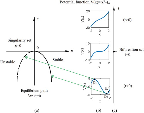
For example, laminar flow is regular (D₁) dominated by viscous. When the velocity increases, which is called control variable change, the flow of fluid begins to be chaotic and vortices occur from D₁ state. At this time, the fluid changes from laminar flow to turbulent flow. Eventually, it will tend to a state of equilibrium – fully developed turbulence (D₂), with the smallest scale of vortices and isotropic turbulence.

The research outline of this method is as follows. First, a suitable catastrophe model is identified on the basis of the type of phase transition and the number of state variables. Second, the main parameters, such as energy and dissipation, which affect the process of phase transition, are selected and written as control variables in a certain function form. Third, the control variables are brought into the critical curve or surface expression to find the quantitative relationship between the parameters. Finally, the critical curve or surface expression is solved to obtain the extremum of different phases.

3. Quantitative catastrophe method analysis of turbulence phase-transition process

Many physicists use wave number to explain the energy transfer in turbulent systems and research the turbulence phase-transition process (Gao, Guo, & Vinen, 2016; Gioia, Ott-Monsivais, & Hill, 2006). Thus, scale and wave number are almost interchangeable concepts, and they are inversely proportional to each other (Adams, Chesler, & Liu, 2014; Cardesa, Vela-Martin, & Jimenez, 2017; Lin & Shen, 2014). Kolmogorov believed that turbulence is composed of vortices of different scales. When the Reynolds number is large enough, the fluid can develop turbulence. Kolmogorov made two famous assumptions: turbulence phase transition is affected by the mean energy dissipation rate ε and the kinematic viscosity ν, considered to be the basis of turbulence research (Frisch, 1995). However, the pulsating energy has never been quantified.

Many researchers have studied turbulence and discovered the law of turbulence, which is the variation of energy fluctuation with time-scale or wave number (Chen, Chen, Eyink, & Sreenivasan, 2003; Falkovich & Ryzhenkova, 1992; Frisch, 1995; Liang, Wu, & Zhong, 2017; Young & Read, 2017). So, the other two important variables for the turbulent phase transition are the energy spectrum (E_k) and time index factor (g) (Frisch, 1995; Layek & Sunita, 2018; Montoya, Nieto, Alvarez, Hernandez, & Jurado, 2018; Romero-Gomez, Harding, & Richmond, 2017).

Therefore, $k$ is regarded as the state variable; $\epsilon$(L²T⁻³), $\nu$(L²T⁻¹), and the energy spectrum density $E_k$(L³T⁻²) are identified as the control variables; and $t$ is in the power exponent form in accordance with $E_{kk}=C_k{\epsilon }^{2/3}{k}^{-5/3}$ and the Reynolds number $Re=LV{\nu }^{-1}$ (Frisch, 1995; Thampi, Doostmohammadi, Shendruk, Golestanian, & Yeomans, 2016): (7) $t=3A{\epsilon }^{g_{\text{1}}}{\nu }^{g_2}{E}_k^g$(7) where A is a constant less than 0; and g₁, g₂, and g denote time-scaling indices.

Thus, the scale index satisfies $\{\begin{array}{l}2g_1+2g_2+3g=-2\\ -3g_1-g_2-2g=0\end{array}$ on the basis of Table 1 and Equations (5(5) $\begin{array}{rl}{V}^{\mathrm{\prime }}(x)& =3x^2+t=0\end{array}$(5) ) and (7(7) $t=3A{\epsilon }^{g_{\text{1}}}{\nu }^{g_2}{E}_k^g$(7) ), and Equation (8(8) $k^2+A{\epsilon }^{(2-g)/4}{\nu }^{(-6-5g)/4}{E}_k^g=0$(8) ) is derived from Equations (5(5) $\begin{array}{rl}{V}^{\mathrm{\prime }}(x)& =3x^2+t=0\end{array}$(5) ) and (7(7) $t=3A{\epsilon }^{g_{\text{1}}}{\nu }^{g_2}{E}_k^g$(7) ): (8) $k^2+A{\epsilon }^{(2-g)/4}{\nu }^{(-6-5g)/4}{E}_k^g=0$(8)

Table 1. Relationship between the scale indices.

	g1 (ε)	g2 (ν)	g (Ek)	t
L	2	2	3	−2
T	−3	−1	−2	0

The expression of energy spectrum density E_k strictly derived from the folding catastrophe model can quantitatively explain the energy in the turbulent system inherited from the large eddies and transferred to the small eddies until viscous dissipation occurs, theoretically and physically. In particular, the energy spectrum density E_k is obtained by Equation (8(8) $k^2+A{\epsilon }^{(2-g)/4}{\nu }^{(-6-5g)/4}{E}_k^g=0$(8) ) as follows: (9) $E_k=-A^{-(1/g)}{\epsilon }^{(g-2)/(4g)}{\nu }^{(5g+6)/(4g)}{k}^{2/g}$(9)

Figure 2 shows various points in the turbulence phase transition: g = −2 (starting stage), g = −9/5 (maximum value), g = −6/5 (derived from $({\mathrm{\partial }}^{2}E)/(\mathrm{\partial }{\nu }^2)=0$, regarded as the singularity set), and g = −2/3 (derived from $({\mathrm{\partial }}^{2}E)/(\mathrm{\partial }{\epsilon }^2)=0$, regarded as the singularity set). g = −2 is the starting point of the change in energy in the turbulence phase transition. g = −9/5 is maximum value for E_k, defined as the energy-containing scale l₀, or the energy-containing wave number k₀ = 1/l₀. According to Kolmogorov’s theory, the range near g = −9/5 is the energy-containing range. In this range, the energy spectrum density increases rapidly, mainly affected by the continuous input of external energy, until the maximum energy spectrum is generated at g = −9/5, reaching its peak. The range near g = −6/5 is the inertial subrange, where $E_{k(g=-6/5)}=-A^{5/6}{\epsilon }^{2/3}{k}^{-5/3}$. The range near g = −2/3 is the dissipation range, where turbulence develops into fully developed turbulence. As explained by folding catastrophe theory, g = −2 is the laminar flow phase, regarded as the unstable equilibrium state, g = −2/3 is the fully developed phase, regarded as the stable equilibrium state, and the range −2 < g < −2/3 is considered as a turbulent development process (transition stage).

Figure 2. (a) Three-dimensional spectrum of energy spectrum density E_k with scale index g and k; (b) change tendency of E_k with changes in g and k; (c) two-dimensional spectrum of E_k with change in k; (d) two-dimensional spectrum of E_k with changes in g.

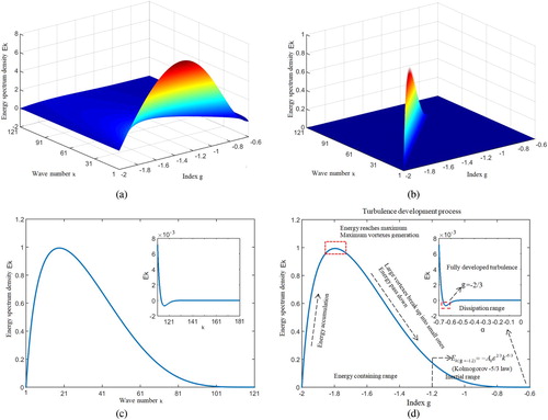
The range near g = −6/5 is the inertial subrange, where $E_{k(g=-6/5)}=-A^{5/6}{\epsilon }^{2/3}{k}^{-5/3}$ is in accord with $E_{kk}=C_k{\epsilon }^{2/3}{k}^{-5/3}$ in Kolmogorov’s theory. The energy-containing range and the inertial subrange are separated, and the inertial subrange and the dissipation range are also separated, as shown in Figure 2, consistent with Kolmogorov’s theory.

This novel turbulence model is a universal form used to study energy in the laminar and turbulence transition process. As an example, a five-stage lifting pump for 6000 m deep-sea mining is simulated and studied, then the turbulent kinetic energy at the outlet with time is extracted to verify this improved model.

4. Model design and mesh generation of five-stage lifting pump

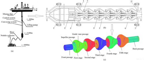
In the 6000 m deep-sea mining system, the multi-stage lifting pump not only provides the power to transport ore, but also ensures that ore can pass through the lifting pump, as the key equipment (Han, Wang, Wu, Liu, & Zou, 2002; Yan et al., 2017). A simplified model of the hydraulic pipe lifting system of the lifting pump is shown in Figure 3(a). The pressure energy required to lift the mixed fluid from the intermediate bin (−5100 m) to the sea surface is provided solely by the lifting pump.

Figure 3. (a) Simplified model of hydraulic pipe lifting system for a lifting pump; (b) structural diagram of five-stage lifting pump: 1 = import flange; 2 = motor; 3 = motor barrel; 4 = impeller; 5 = space guide vane; 6 = five-stage lifting pump barrel; 7 = export flange; 8 = ring flow channel; 9 = pump inlet flange; 10 = pump outlet flange; (c) three-dimensional mesh model of five-stage lifting pump.

4.1. Flow design method of five-stage lifting pump

According to a research report on sea mining test systems (Zou, 2007), the main technical indicators of a mining system are: the output of dry nodules is W_g = 30 t/h; according to the water content of the nodules, the output of wet nodules is W_s = 45 t/h; the concentration of ore transported $C_v=5\sim 10\mathrm{\%}$; the density of polymetallic nodules ${\rho }_s=2040\text{kg/}{\text{m}}^3$; the average diameter of nodules $d_s=20\sim 50\text{mm}$; the density of seawater ${\rho }_l=1025\text{kg/}{\text{m}}^3$; and the depth of intermediate storage in a 6000 m deep-sea mining system is $L=5400\text{m}$. The production capacity of the mining system can be determined by these technical indicators, and the workflow of the conveying system can be obtained.

The volume flow rate of ore Q_s is: (10) $Q_s=\frac{W_s}{t{\rho }_s}$(10) where ${\rho }_s$ is density ($\text{kg/}{\text{m}}^3$), and the output of wet nodules within time t₀ is W_s.

The ratio of the volume flow rate Q_s of ore to the volume flow rate Q_m of solid–liquid fluid is the volume concentration C_v: (11) $C_V=\frac{Q_s}{Q_m}$(11)

The solid–liquid flow rate Q_m of the conveying system can be obtained by combining Equations (10(10) $Q_s=\frac{W_s}{t{\rho }_s}$(10) ) and (11(11) $C_V=\frac{Q_s}{Q_m}$(11) ): (12) $Q_m=\frac{W_s}{t{\rho }_s{C}_V}$(12)

It should be noted that the design flow Q of the lifting pump must be greater than the conveying flow Q_m, so that the nodule mining capacity can meet the technical indicators.

The density of solid–liquid is the mass of solid–liquid fluid per unit volume: (13) ${\rho }_m=\frac{{\rho }_l{Q}_l+{\rho }_s{Q}_s}{Q_m}$(13) where $Q_l$ is volume flow of seawater (${\text{m}}^3\text{/h}$); $Q_s$ is the volume flow of solid and liquid fluids (${\text{m}}^3\text{/h}$); and $Q_m$ is the volume flow of solid and liquid fluids (${\text{m}}^3\text{/h}$). (14) $Q_m=Q_l+Q_s$(14) Therefore, (15) ${\rho }_m=C_V{\rho }_s+(1-C_V){\rho }_l$(15)

According to the theory of particle sedimentation, the sedimentation velocity of solid particles $u_t$ is: (16) $u_t=\sqrt{\frac{\pi d_{s}g({\rho }_s-{\rho }_l)}{6\phi {\rho }_l}}$(16) where $\phi$ is the spherical drag coefficient, and its drag coefficient $\phi =(\pi /8)C$, $C=0.4\sim 0.5$; and $d_s$ is the average diameter of ore particles (mm). So, (17) $u_t=\sqrt{\frac{8}{3}{d}_{s}g\left(\frac{{\rho }_s-{\rho }_l}{{\rho }_l}\right)}$(17)

Considering that the shape of solid ore is polygonal, a shape coefficient $\psi$ is introduced, where $\psi =0.67\sim 0.82$. Equation (17(17) $u_t=\sqrt{\frac{8}{3}{d}_{s}g\left(\frac{{\rho }_s-{\rho }_l}{{\rho }_l}\right)}$(17) ) can be converted to: (18) $u_t=(0.67\sim 0.82)\sqrt{\frac{8}{3}{d}_{s}g\left(\frac{{\rho }_s-{\rho }_l}{{\rho }_l}\right)}$(18)

According to Govier's theory (Zou, 2007), the axial velocity of solid–liquid flow must be at least twice that of ore settling to ensure the system's ability to transport nodules.

4.2. Head design method of five-stage lifting pump

The first phase is seawater, and the second phase is the formation of ore particles.

The Bernoulli equation in the lifting system is: (19) $\begin{array}{r}\frac{P_1}{{\rho }_{m}g}+{\alpha }_{m1}\frac{u_{m1}^2}{2g}+Z_1=\frac{P_2}{{\rho }_{m}g}+{\alpha }_{m2}\frac{u_{m2}^2}{2g}+Z_2+\mathrm{\Delta }{h}_m\end{array}$(19) where $P_1\text{ and }{P}_2$ are the pressures corresponding to sections 1 and 2, respectively (Pa); ${\alpha }_{m1}$ and ${\alpha }_{m2}$ are kinetic energy correction factors for sections 1 and 2; $u_{m1}$ and $u_{m2}$ are the average flow rates in sections 1 and 2; $Z_1$ and $Z_2$ are the vertical distances between sections 1 and 2; and ${\rho }_m$ is solid–liquid fluid density (${\rho }_m=C_v\times {\rho }_s+(1-C_v)\times {\rho }_l$).

The multi-stage lifting pump provides the required pressure energy to lift the mixed fluid from the intermediate bin to the surface of mining ship (Figure 3), so Equation (19(19) $\begin{array}{r}\frac{P_1}{{\rho }_{m}g}+{\alpha }_{m1}\frac{u_{m1}^2}{2g}+Z_1=\frac{P_2}{{\rho }_{m}g}+{\alpha }_{m2}\frac{u_{m2}^2}{2g}+Z_2+\mathrm{\Delta }{h}_m\end{array}$(19) ) can be calculated as: (20) $\begin{array}{r}{H}_{min}{\rho }_{w}g+{\rho }_{l}gL=P_{out}+{\rho }_{m}gL+\mathrm{\Delta }{h}_m+\frac{{\rho }_m{u}_{out}^2}{2}\end{array}$(20) where $H_{min}$ is the minimum head required; ${\rho }_w$ is water density; ${\rho }_m$ is mixed fluid density; $u_{out}$ is the mixed fluid flow velocity at the outlet of the hard pipe for mine lifting; and $P_{out}$ is the pressure at the outlet of the hard pipe. So, Equation (20(20) $\begin{array}{r}{H}_{min}{\rho }_{w}g+{\rho }_{l}gL=P_{out}+{\rho }_{m}gL+\mathrm{\Delta }{h}_m+\frac{{\rho }_m{u}_{out}^2}{2}\end{array}$(20) ) can be calculated as: (21) $H_{min}=\frac{P_{out}}{{\rho }_{w}g}+\frac{{\rho }_{m}L}{{\rho }_w}-\frac{{\rho }_{l}L}{{\rho }_w}+\frac{{\rho }_m{u}_{out}^2}{2{\rho }_{w}g}+\frac{\mathrm{\Delta }{P}_m}{{\rho }_{w}g}$(21) where $P_{out}/({\rho }_{w}g)$ is the pressure energy at the outlet; $({\rho }_{m}L)/{\rho }_w$ is the potential energy of solid–liquid fluid; $({\rho }_{l}L)/{\rho }_w$ is the potential energy of seawater; $({\rho }_m{u}_{out}^2)/(2{\rho }_{w}g)$ is the kinetic energy of solid–liquid fluid at the outlet; and $(\mathrm{\Delta }{P}_m)/({\rho }_{w}g)$ is hydraulic loss of solid–liquid fluid in the pipeline.

The higher the speed, the higher the head of the multi-stage pump and the lower the efficiency. The choice of speed has a large effect on the wear of the components and the vibration of the lifting pump system. Through simulation, we found that n = 1450 rpm is the most appropriate rotation speed.

In summary, the working performance of the multi-stage pump is small flow, high lift. The multi-stage pump is designed by the amplifying flow design method to enlarge the flow channel width of the lifting pump, and the working flow is lower. Therefore, the design flow of the multi-stage pump is $Q=800{\text{m}}^3\text{/h}$ and the design speed is $n=1450\text{rpm}$, The design head of the single-stage pump is H = 35 m; therefore, the design head of the five-stage pump is $H_5$ = 175 m. Four sets of five-stage pulp pumps are connected in series in the 6000 m mining system. The lifting pump is a segmental multi-stage centrifugal pump and its structure is shown in Figure 3(b).

4.3. Computer-aided design method of blades of impeller and guide vane

The design method of the impeller blade is as follows.

The inlet diameter of impeller D_j is calculated as: (22) $D_j=\sqrt{{\left(K_0\sqrt[3]{\frac{Q}{n}}\right)}^2+D_h^2}$(22) where K₀ is the empirical coefficient, K₀ = 3.8∼4.5; and D_h is the hub diameter.

The outer diameter D₂ of the impeller is as follows: (23) $D_2=(9.35\sim 9.6){\left(\frac{n_s}{100}\right)}^{-0.5}\sqrt[3]{\frac{Q}{n}}$(23) where $n_s=(3.65n\sqrt{Q})/H^{3/4}$.

The blade width b₂ at the impeller exit is: (24) $b_2=(1.0\sim 1.4){\left(\frac{n_s}{100}\right)}^{5/6}\sqrt[3]{\frac{Q}{n}}$(24)

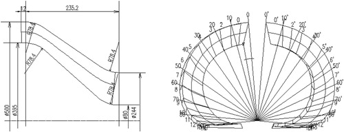
The blade profile is designed by the logarithmic helix equation, as follows: (25) $r=r_1{e}^{\theta \left[\frac{\tan {\beta }_2-\tan {\beta }_1}{K+1}{\left(\frac{\theta }{{\phi }_1}\right)}^K+\tan {\beta }_1\right]}$(25) where θ is the polar angle; K is the empirical coefficient, where $K=\frac{(\tan {\beta }_2-\tan {\beta }_1)\phi }{\ln (r_2/r_1)}-\phi \tan {\beta }_1-1$; $r_1$ is the impeller inlet radius; and $r_2$ denotes the impeller exit radius.

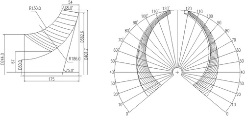
The number of blades Z_i is generally 3–6, and the wrap angle of blade is generally 85–150°. When the number of blades is large, the blade wrap angle takes a small value. The larger the inlet angle β₁ of the blade, the larger the flow area of the impeller inlet, and the wear of the blade at the entrance is reduced. So, β₁ generally takes a value of 20–40°. The blade exit angle β₂ is generally taken to be 10–30° in consideration of wear at the blade at the exit. The wooden patterns of the impeller blade are shown in Figure 4.

Figure 4. Wooden patterns of the impeller blade.

The guide vane is an important energy-conversion component, and its blade design method is as follows.

The maximum diameter D₃ of the inner streamline is $D_3=D_2+(2\sim 5)$, where D₂ is the outer diameter of the impeller. The maximum diameter D₄ of the outer streamline is $D_4=(1.2\sim 1.45)D_2$. The axial length L is $L=(0.5\sim 0.7)D_2$. The number of guide vanes is $Z=Z_{\text{i}}\pm 1$. The inlet angle of the blade of the guide vane is ${\alpha }_3={\alpha }_3^{\mathrm{\prime }}+\mathrm{\Delta }\alpha$, where $\mathrm{\Delta }\alpha =3^{\circ }\sim {10}^{\circ }$ and ${\alpha }_3^{\mathrm{\prime }}=\arctan (v_{m3}/v_{u3})$. The outlet angle of the blade of the guide vane is ${\alpha }_4=80\sim {95}^{\circ }$. The blade profile is designed by $d_{\phi }=(1/r\tan a)d_l$. Its wooden patterns are shown in Figure 5.

Figure 5. Wooden patterns of the guide vane blade.

The main geometric parameters of the blades of the impeller and space guide vane are listed in Table 2.

Table 2. Main geometric parameters of blades.

Impeller	Value	Space guide vane	Value
Inlet diameter Dj (mm)	224	Inner streamline diameter D3 (mm)	395
Wrap angle ϕ1 (°)	120	Wrap angle ϕ2 (°)	90
Impeller diameter D2 (mm)	401.7	Axial length L (mm)	235.2
Blade inlet angle β1 (°)	28	Blade inlet angle α3 (°)	12
Blade number Z1	3	Blade number Z2	4
Blade outlet angle β2 (°)	22	Blade outlet angle α4 (°)	90
Outlet width b2 (mm)	54	Outer streamline diameter D4 (mm)	500

For the convenience of installation, the motor and the multi-stage lifting pump are fixed, respectively, in the motor cylinder and the pump barrel. The import and export flanges, the motor barrel, and the pump barrel are fixed on the same axis by the bolt. The import and export flanges are connected with the lifting hard pipe in series, as shown in Figure 3(b).

4.4. The spatial discretization process

The calculation area of the lifting pump includes the inlet and outlet extension section (static zone), the impeller passage (rotating zone), and the space guide vane passage (static zone).

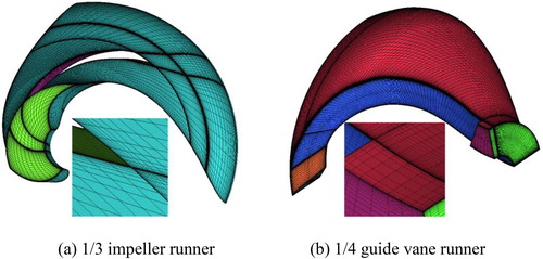
This model uses structured mesh to improve the accuracy of the simulation. According to the number of blades, the structured grids of the 1/3 impeller runner and 1/4 guide vane runner are made as shown in Figure 6(a) and (b). Closer to the walls and boundary layers, denser grids are used to improve the simulation accuracy. The first layer grids for the walls and boundaries are at $\mathrm{\Delta }y=0.0005$, guaranteeing that the first layer grids for the wall are situated nearly everywhere at $y^{+}=u_{\ast }\mathrm{\Delta }y/\nu =1.0$. More than two grid faces are made in the laminar subregion (y⁺ < 5.0).

Figure 6. Computational grid: (a) 1/3 impeller runner; (b) 1/4 guide vane runner.

4.5. Mathematical models and the numerical algorithm

We verified the accuracy of the new turbulence model based on catastrophe theory and Kolmogorov’s theory, by comparing the energy changes between the traditional numerical simulation method and the new turbulence model.

4.5.1. Mathematical models

Mou, He, Zhao, and Chau (2017) present the effects of wind on various square high-rise buildings in detail using computational fluid dynamics (CFD) technology. In Mosavi et al. (2019), the multi-input bubble column reactor is simulated and predicted based on the hybrid model of CFD. Consequently, this paper adopts the k–ε turbulence model and the Navier–Stokes equations, including the continuity equation and the momentum equation (Issakhov, Bulgakov, & Zhandaulet, 2019). (26) $\begin{array}{rl}\mathrm{\partial }{u}_j\text{/}\mathrm{\partial }{x}_j& =0\end{array}$(26) (27) $\begin{array}{rl}\frac{\mathrm{\partial }{u}_i}{\mathrm{\partial }t}+\frac{\mathrm{\partial }}{\mathrm{\partial }{x}_j}(u_i{u}_j)& =-\frac{1}{\rho }\frac{\mathrm{\partial }P}{\mathrm{\partial }{x}_i}\\ & +\frac{\mathrm{\partial }}{\mathrm{\partial }{x}_j}\left[{\mu }_{eff}\left(\frac{\mathrm{\partial }{u}_i}{\mathrm{\partial }{x}_j}+\frac{\mathrm{\partial }{u}_j}{\mathrm{\partial }{x}_i}\right)\right]+f_i\end{array}$(27)

The kinematic relationship between the position and the velocity of particles is as follows: (28) $\begin{array}{rl}d{x}_p/d_t& =u_p\end{array}$(28) (29) $\begin{array}{rl}{m}_p\frac{d{u}_p}{d_t}& =F_D+F_G\end{array}$(29)

Four turbulence models are determined for testing:

1. The k–ε turbulence model consists of an eddy viscosity and two equations (Jones & Launder, 1972): (30) $\begin{array}{rl}\frac{\mathrm{\partial }(\rho k)}{\mathrm{\partial }t}+\frac{\mathrm{\partial }(\rho k{u}_j)}{\mathrm{\partial }{x}_j}& =\frac{\mathrm{\partial }}{\mathrm{\partial }{x}_j}\left[\left(\mu +\frac{{\mu }_t}{{\sigma }_k}\right)\frac{\mathrm{\partial }k}{\mathrm{\partial }{x}_j}\right]\\ & +P_k-\rho \epsilon +P_{kb}\end{array}$(30) (31) $\begin{array}{rl}\frac{\mathrm{\partial }(\rho \epsilon )}{\mathrm{\partial }t}+\frac{\mathrm{\partial }(\rho \epsilon u_j)}{\mathrm{\partial }{x}_j}& =\frac{\mathrm{\partial }}{\mathrm{\partial }{x}_j}\left[\left(\mu +\frac{{\mu }_t}{{\sigma }_{\epsilon }}\right)\frac{\mathrm{\partial }\epsilon }{\mathrm{\partial }{x}_j}\right]\\ & +\frac{\epsilon }{k}(C_{1\epsilon }{P}_k-C_{2\epsilon }\rho \epsilon +C_{1\epsilon }{P}_{\epsilon b})\end{array}$(31) where constants are defined as follows (Launder & Spalding, 1974):$C_{1\epsilon }=1.44,C_{2\epsilon }=1.9,{\sigma }_{\epsilon }=1.2,{\sigma }_k=1,C_3=1$.

2. The shear stress transport (SST) k–ω turbulence model (Goldberg & Batten, 2015; Hu et al., 2016) consists of an eddy viscosity and two equations. Because the turbulence model inside the boundaries allows it to be directly related to the wall by the viscous layer, the SST k–ω turbulence model is available to the low Reynolds turbulence model without adding damping functions. (32) $\begin{array}{rl}\frac{\mathrm{\partial }(\rho k)}{\mathrm{\partial }t}+\frac{\mathrm{\partial }(\rho k{u}_j)}{\mathrm{\partial }{x}_j}& =\frac{\mathrm{\partial }}{\mathrm{\partial }{x}_j}\left[\left(\mu +\frac{{\mu }_t}{{\sigma }_k}\right)\frac{\mathrm{\partial }k}{\mathrm{\partial }{x}_j}\right]\\ & +P_k-{\beta }^{\ast }\rho k\omega +P_{kb}\end{array}$(32) (33) $\begin{array}{rl}\frac{\mathrm{\partial }(\rho \omega )}{\mathrm{\partial }t}+\frac{\mathrm{\partial }(\rho \omega u_j)}{\mathrm{\partial }{x}_j}& =\frac{\mathrm{\partial }}{\mathrm{\partial }{x}_j}\left[\left(\mu +\frac{{\mu }_t}{{\sigma }_{\omega }}\right)\frac{\mathrm{\partial }\omega }{\mathrm{\partial }{x}_j}\right]\\ & +\alpha \frac{\omega }{k}{P}_k-\beta \rho k{\omega }^2+P_{\omega b}\end{array}$(33) where the constants have the following values (Wilcox, 1988):

   ${\sigma }_k=2,{\sigma }_{\omega }=2,\beta =0.075,{\beta }^{\ast }=0.09,\alpha =5/9.$

3. The detached eddy simulation (DES) model (Haque, Katsuchi, Yamada, & Nishio, 2016; Tang et al., 2015) is combined with the RANS (calculating the near-wall parts) and LES (calculating the remaining areas) for numerical simulation: $\epsilon =\beta \ast k\omega =k^{3/2}/L_t\to k^{3/2}/(C_{\text{DES}}\Delta )$ $\text{for}(C_{\text{DES}}\mathrm{\Delta }<L_t)$ $\Delta =\text{max}(\Delta i);L_t=(\sqrt{k})/\beta \ast \omega$

The DES revision is expressed as a factor in the destructive term in the k equation (Issakhov, Zhandaulet, & Nogaeva, 2018): $\epsilon =\beta \ast k\omega \to \beta \ast k\omega \bullet F_{\text{DES}}$where $F_{\text{DES}}=\text{max}\left(\frac{L_t}{C_{\text{DES}}},1\right)\text{and }{C}_{\text{DES}}=0.61$

1. Turbulence involves a wide variety of scales. The LES can solve large-scale fluctuating motions and use the subnet-scale turbulent model for small-scale eddies (Issakhov, 2017).

4.5.2. The numerical algorithm

As a numerical algorithm, the semi-implicit method for pressure-linked equations (SIMPLE) has proved to be successful in solving some numerical solution problems of Equations (26(26) $\begin{array}{rl}\mathrm{\partial }{u}_j\text{/}\mathrm{\partial }{x}_j& =0\end{array}$(26) ) and (27(27) $\begin{array}{rl}\frac{\mathrm{\partial }{u}_i}{\mathrm{\partial }t}+\frac{\mathrm{\partial }}{\mathrm{\partial }{x}_j}(u_i{u}_j)& =-\frac{1}{\rho }\frac{\mathrm{\partial }P}{\mathrm{\partial }{x}_i}\\ & +\frac{\mathrm{\partial }}{\mathrm{\partial }{x}_j}\left[{\mu }_{eff}\left(\frac{\mathrm{\partial }{u}_i}{\mathrm{\partial }{x}_j}+\frac{\mathrm{\partial }{u}_j}{\mathrm{\partial }{x}_i}\right)\right]+f_i\end{array}$(27) ) for the calculation of incompressible fluid flow. The entrance boundary condition is velocity inlet $v_0=(Q/A)=(4Q/\pi D_1^2)$, and the outflow is used for the outlet boundary condition. The standard wall functions are used to calculate the influence of the walls on flow (Launder & Spalding, 1974). Equations (28(28) $\begin{array}{rl}d{x}_p/d_t& =u_p\end{array}$(28) ) and (29(29) $\begin{array}{rl}{m}_p\frac{d{u}_p}{d_t}& =F_D+F_G\end{array}$(29) ) were computed by Euler implicit discretization, and the additional Equations (30(30) $\begin{array}{rl}\frac{\mathrm{\partial }(\rho k)}{\mathrm{\partial }t}+\frac{\mathrm{\partial }(\rho k{u}_j)}{\mathrm{\partial }{x}_j}& =\frac{\mathrm{\partial }}{\mathrm{\partial }{x}_j}\left[\left(\mu +\frac{{\mu }_t}{{\sigma }_k}\right)\frac{\mathrm{\partial }k}{\mathrm{\partial }{x}_j}\right]\\ & +P_k-\rho \epsilon +P_{kb}\end{array}$(30) ) and (31(31) $\begin{array}{rl}\frac{\mathrm{\partial }(\rho \epsilon )}{\mathrm{\partial }t}+\frac{\mathrm{\partial }(\rho \epsilon u_j)}{\mathrm{\partial }{x}_j}& =\frac{\mathrm{\partial }}{\mathrm{\partial }{x}_j}\left[\left(\mu +\frac{{\mu }_t}{{\sigma }_{\epsilon }}\right)\frac{\mathrm{\partial }\epsilon }{\mathrm{\partial }{x}_j}\right]\\ & +\frac{\epsilon }{k}(C_{1\epsilon }{P}_k-C_{2\epsilon }\rho \epsilon +C_{1\epsilon }{P}_{\epsilon b})\end{array}$(31) ) or (32) and (33) were computed by explicit time discretization. All calculations were completed in ANSYS FLUENT. Designs were produced on a personal computer (Intel^® Core™ CPU i5-7500, 3.40 GHz, 8 GB RAM) and ?>simulations were performed in the cluster system (Intel^® Xeon^® CPU E5-2670, 2.50 GHz, 128 GB RAM) to save computing time.

5. Numerical simulation results and analysis at the fully developed turbulence stage based on the universal turbulence model

Under the conditions of rotation speed $n=1450\text{rpm}$, particle size $d=30\text{mm}$, and concentration $C_v=8\mathrm{\%}$, the solid–liquid two-phase flow field with different flow rates, 420, 560, and 700 m³/h, is numerically simulated. To verify the universal turbulence model, the particle clogging problem and the hydraulic performance of the new designed lifting pump are studied through the analysis of velocity distribution and pressure distribution at the fully developed turbulence stage.

5.1. Velocity distribution of full flow runner with different flow rates

From the velocity distribution, we can directly see the efficiency, trajectories, and outflow time of solid particles. The velocity distributions of the flow field in five-stage pumps with different flow rates (Q = 420, 560, and 700 m³/h) are shown in Figure 7(a)–(c).

Figure 7. Velocity distribution of flow field in the five-stage lifting pump: (a) Q = 420 m³/h; (b) Q = 560 m³/h; (c) Q = 700 m³/h.

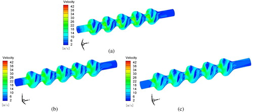
The impeller accelerates the solid–liquid flow to provide kinetic energy. The maximum velocity in the whole flow path appears at the tail of the impeller passage. The fluid with maximum flow velocity flows out of the impeller runner and flows into the space guide vane flow passage through the steering action of the outer cover plate. The velocity of the solid liquid flow decreases rapidly in the space guide vane region.

The speed at the impeller exit exceeds 30 m/s, so the rotating acceleration effect of the impeller blade on solid–liquid flow is obvious, as shown in Figure 7(a). The movement of the particles is smooth and the blade design is reasonable. The velocity difference of the space guide vane is over 20 m/s, so the effect of the diffuser is improved.

Comparison of the velocity nephograms in Figure 7(a)–(c) reveals that the particle trajectory becomes more stable as the velocity increases. Stable particles are not susceptible to turbulence of water flow, so the length of the actual trajectory is shorter. On the other hand, as the velocity increases, the time required for particles to flow through the same distance is shorter, which reduces the outflow time for particles. A stable trajectory and shorter outflow time will improve the blockage situation. The smaller the work flow, the less serious the blockage.

The design of the amplification flow method and working at a smaller flow rate can enlarge the width of the impeller flow path and improve the flow capacity of particles, so the performance of the lifting pump can be improved.

5.2. Pressure distribution in full flow passage with different flow rates

If there is a blockage of solid particles, the pressure and the energy transfer of the impeller will be affected, and then the performance of the lifting pump will be affected. The nephograms of the absolute pressure distribution in the five-stage pump with different flow rates (Q = 420, 560, and 700 m³/h) are shown in Figure 8(a)–(c).

Figure 8. Pressure distribution of flow field in the five-stage lifting pump: (a) Q = 420 m³/h; (b) Q = 560 m³/h; (c) Q = 700 m³/h.

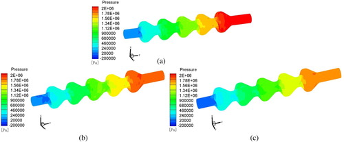
The pressure of the flow field is obviously increased from the inlet to the outlet, as shown in Figure 8(a). There is no large low-pressure area at the impeller inlet area.

Comparing the nephograms in Figure 8, with the increase in the lifting pump series, the pressure increases sharply, as shown in Figure 8(a). Therefore, the energy transfer effect of the space guide vane is improved. As the flow decreases, the absolute pressure at the outlet is significantly greater, as shown in Figure 8(a)–(c). Under the condition in Figure 8(a), the absolute pressure at the outlet exceeds 2000 kPa, while the absolute pressure in Figure 8(b) is close to 2000 kPa. Under the condition in Figure 8(c), the absolute pressure at the outlet is significantly less than 2000 kPa. The pressure difference is up to 2000 kPa, which can satisfy the requirements for lifting. Therefore, these conditions are favorable for the transport of solid particles at a lower flow rate.

5.3. Axial velocity distribution of Z axis of Y section with different flow rates

The main function of the five-stage lifting pump is to transport solid metal particles, so the axial velocity is one of the important parameters of a lifting pump. The axial velocity also reflects the efficiency of the lifting pump. The lifting pump is a central symmetrical structure. The positive direction of the Z axis is in accordance with the flow direction. The axial velocity distributions of the Z axis of the Y section under different flow conditions (Q = 420, 560, and 700 m³/h) in the five-stage pump are shown in Figure 9(a)–(c). In the impeller passage, the maximum axial speed is 12 m/s, and the water flow can transport solid particles more effectively. So, the linear design of the impeller blade is reasonable.

Figure 9. Axial velocity distribution of the five-stage lifting pump: (a) Q = 420 m³/h; (b) Q = 560 m³/h; (c) Q = 700 m³/h.

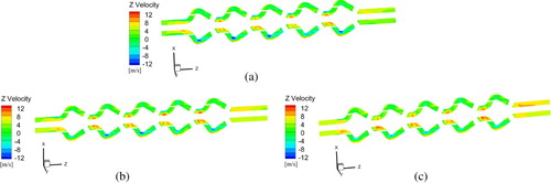
Under the condition of high flow rates, the axial velocity in the impeller passage and the guide vane passage is slightly larger than for the low flow-rate condition in Figure 9(a)–(c). With the increase in axial speed, the lifting power is stronger and efficiency is improved. So, the work flow should not be too small.

5.4. Pressure distribution of impeller blade pressure surface with different flow rates

During the operation of the five-stage pump, the solid–liquid fluid obtains kinetic energy under the rotation of the blade. The blade pressure distribution can reflect the effect of the impeller on solid–liquid fluid. Absolute pressure distributions of the impeller blade pressure surface under different flow conditions (Q = 420, 560, and 700 m³/h) in the five-stage pump flow field are shown in Figure 10(a)–(c). As the radial radius of the blade increases, the transmission force to the solid–liquid flow increases, and the pressure of the blade increases. The pressure gradient is approximately perpendicular to the central axis of the five-stage pump, and the pressure field on the blade changes uniformly, so the solid particles move smoothly, and the function of impeller is effective. The blade linear design is reasonable, and the energy transfer is more efficient.

Figure 10. Pressure distribution of impeller blade pressure surface: (a) Q = 420 m³/h; (b) Q = 560 m³/h; (c) Q = 700 m³/h.

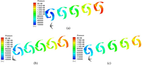
The pressure increases sharply as the flow rate decreases. Under the condition in Figure 10(a), the pressure value of the blade pressure surface at the pump outlet is more than 2000 kPa, whereas pressure in Figure 10(b) is close to 2000 kPa, and the absolute pressure under the condition in Figure 10(c) is less than 2000 kPa. Under the condition of large flow rate, the movement of solid particles is prone to disorder, which directly affects the pressure effect of the lifting pump impeller on solid–liquid flow and the hydraulic performance of the lifting pump. As can be seen from Figure 10, the hydraulic performance of the five-stage lifting pump is best under the condition of Q = 420 m³/h.

5.5. Velocity vector pictures of Z cross-section with different flow rates

The velocity vector pictures of the five-stage lifting pump under different flow conditions (Q = 420, 560, and 700 m³/h) are shown in Figure 11(a)–(c). From the surface vector diagram of the impeller blade, we can see the specific trend of the particles in the three-dimensional space of the pump chamber. The fifth stage pressure distribution is the largest in Figures 7 and 8, so we only take the fifth stage pump to study the velocity vector of the Z cross-section.

Figure 11. Velocity vector images of Z cross-section: (a) Q = 420 m³/h; (b) Q = 560 m³/h; (c) Q = 700 m³/h.

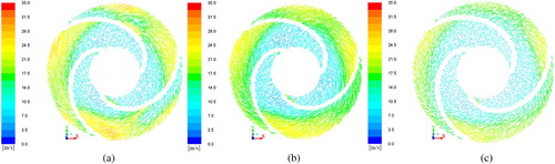
Along the inlet of the impeller to the exit, the relative velocity of solid–liquid flow increases gradually, and the whole flow line is smooth. There is no large area of velocity gradient, no flow phenomenon occurs, and there is no large eddy. This shows that the design of the impeller blade is reasonable, in general. Particles in the impeller move along with the liquid, so the movement of solid particles is improved, and their movement is basically the same. There are no obvious eddies or reflux in the area, and there is no jet wake structure. Energy loss is very small. The numerical simulation preferably reflects the actual change in the relative velocity. The performance of the impeller is good for the solid–liquid flow, and the efficiency and hydraulic efficiency of the five-stage pump are improved. The blade linear design of the pump with the enlarged flow design method is reasonable, and it can work well under different flow conditions.

6. Simulation verification of turbulent flow energy derived by the improved method

Figure 12 shows the variation in the turbulent kinetic energy spectrum with time in the process of turbulence formation. The abscissa is time factor (t_s). The turbulent kinetic energy spectrum E_k under different flow conditions is shown in Figure 9. We can see that the E_k varies with time. The highest point of the turbulent kinetic energy spectrum is t_s = 2. With t_s from 0 to 1, the region is called the large eddy range; with t_s from 1 to 5.6, the region is the energy-containing range; with t_s from 5.6 to 8.8, the region is the inertial subrange; with t_s from 4 to 8.8, the region is called the dissipation range; and after 8.8, the system reaches fully developed turbulence. These values are in accordance with the changing trends derived from Equation (9(9) $E_k=-A^{-(1/g)}{\epsilon }^{(g-2)/(4g)}{\nu }^{(5g+6)/(4g)}{k}^{2/g}$(9) ). One of the important characteristics of catastrophe theory is that it can quantitatively predict the phase transition of a system even without knowing the differential equation of the system. The numerical results of turbulence transformation obtained by catastrophe theory are in agreement with the numerical simulation of the differential equations.

Figure 12. Comparison of the turbulent kinetic energy spectrum under various flow conditions and theoretical derivation values in the flow field from the 1/2 exit in the back passage: (a) Q = 420 m³/h; (b) Q = 560 m³/h; (c) Q = 700 m³/h.

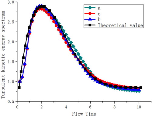
Figure 12 shows the variation in the turbulent kinetic energy spectrum with the time-scale factor at different points. Time is the reciprocal of frequency, and the relationship between frequency and wave number is $k=2\pi f_i/u_i$. Figure 2 shows that the wave number k and index g are in one-to-one correspondence, so the 2 point on the abscissa of Figure 9 is consistent with the g = −1.8 point of theoretical deduction in Figure 2. The energy of the fluid system increases gradually, and positive energy accumulation occurs in the region of −2 < g < −1.8, that is, 0–2 in Figure 12. In the region of −1.8 < g, i.e. where the time t_s is greater than 2 in Figure 12, the amount of energy dissipated is greater than the amount obtained from the outside, so there is a negative accumulation of energy. At this point, the large-scale vortex gradually ruptures and forms a small-scale vortex, and transfers energy to the small-scale vortex. In this way, we prove the accuracy of this turbulence model in the five-stage lifting pump for the 6000 m deep-sea mining system.

7. Test verification

The School of Mechanical and Electrical Engineering of Central South University and the Research Institute of Mining and Metallurgy jointly established the State Key Laboratory for deep-sea mineral resource exploitation and utilization. The laboratory has vertical deep-sea mining lift test equipment equipped with flow, pressure, and ore volume fraction testing equipment for lifting transportation. The experimental equipment simulates the deep-sea pressure environment by adding back-pressure at the output. Part of the experimental equipment is shown in Figures 13 and 14.

Figure 13. Water supply pipe.

Figure 14. Lifting pump.

7.1. Simulated calculation method of head and efficiency

The total pressure difference is the pump head, and the calculation formula for the predicted head of the pump is as follows: (34) $\begin{array}{rl}{H}_m& =\frac{1}{A_b}{\int }_{A_b}\left(\frac{p_b}{{\rho }_{m}g}+\frac{v_b^2}{2g}\right)d_A\\ & -\frac{1}{A_a}{\int }_{A_a}\left(\frac{p_a}{{\rho }_{m}g}+\frac{v_a^2}{2g}\right)d_A\end{array}$(34) where A_a and A_b are the inlet and outlet area of the lifting pump; p_a, p_b are the inlet pressure and outlet pressure; and v_a and v_b are the inlet and outlet velocities, respectively. So, (35) $H_m=\frac{p_{mb}-p_{ma}}{{\rho }_{m}g}+\mathrm{\Delta }z$(35) where $p_{ma}$ is the total pressure of the outlet section; and $\mathrm{\Delta }z$ is the vertical distance of the inlet and outlet sections.

The hydraulic efficiency formula of the lifting pump is as follows: (36) ${\eta }_m=\frac{{\rho }_{m}gQ{H}_m}{M\omega }\times 100\mathrm{\%}$(36) where M is the impeller torque; and ω is the impeller angular velocity.

7.2. Test calculation method of head and efficiency

The total pressure difference is the pump head, ignoring the total head loss of the inlet and outlet. The formula for calculating the experimental head of the lifting pump is as follows: (37) $H=\frac{p_b-p_a}{{\rho }_{m}g}+\frac{v_b^2-v_a^2}{2g}+\mathrm{\Delta }z$(37) where $p_b$ and $p_a$ are values of the outlet and inlet pressure gauge; $v_b$ is average velocity at the outlet section, $v_b=(Q/A_b)$; $v_a$ is average velocity at the inlet section; and $v_a=(Q/A_a)\mathrm{\Delta }z$ is the distance from the center position of the pressure gauge to the inlet and outlet in the vertical direction, where $\mathrm{\Delta }z=4.8m$.

The experimental efficiency calculation formula of the lifting pump is as follows: (38) $\eta =\frac{P_B}{P_M}\times 100\mathrm{\%}$(38) where $P_B$ is the effective power of the pump, $P_B=({\rho }_{m}gQH/3600)\times {10}^{-3}$; and $P_M$ is motor power, $P_M=2\pi n_w\cdot M_w$.

The single-stage lifting pump was installed in the pump test platform to check the correctness of the simulation through experimentation. The pressure transmitter, torque sensor, and torque measuring instrument were used to measure the pressure of the pump, the rotation shaft torque, and the rotation speed, respectively. The measured head (H) and efficiency (η) curves and the numerical simulation results are compared in Figure 15. The hollow triangles and squares represent the simulated values, and the solid triangles and squares represent test values. The error mainly concerns energy loss at clearance joints, dynamic–static joints, and bearings. The numerical calculations are basically in accordance with the test results, which proves the feasibility and accuracy of the numerical simulation method.

Figure 15. Head and efficiency curves between numerical simulation results and experimental results: 1 = head simulation value; 2 = head test value; 3 = efficiency simulation value; 4 = efficiency test value.

8. Conclusions

1. The universal process of turbulence formation can be exactly derived based on catastrophe theory and non-dimensional analysis. This method can quantitatively analyze the relationship between the energy pulsation spectrum and wave number with respect to a time index factor g to explain the energy in the turbulent system inherited from the large eddies and transferred to the small eddies until viscous dissipation occurs, theoretically and physically.

2. For the universal turbulence model, solid–liquid two-phase flow in a five-stage lifting pump in the fully developed turbulence stage is studied. The outlet velocity of the impeller is up to 30 m/s, so the linear design of the blade is reasonable for the new design pump. The smaller the work flow, the less serious the blockage. The design of the amplification flow method and working at a smaller flow rate can ameliorate the flow capacity of particles and the function of the lifting pump. The pressure difference is up to 2000 kPa, which can satisfy the requirement of lift. It is conducive to the improvement of the particle blocking problem to work with a small flow rate.

3. Comparing the turbulent kinetic energy and theoretical deduction under different flow conditions, it is found that the theoretical deduction is consistent with the simulation results.

4. Our method provides equations that enable a quantitative analysis with a physical explanation for turbulence formation, which not only provides new insight into turbulence, but also can be applied to other complex phase transitions.

5. The particle shape of polymetallic nodules is irregular and the range of particle sizes varies greatly. In the simulation and experiment, we assume that nodules are single spherical particles. In future research, assuming improved computing capability, we could introduce multiple phases and solve multiple Euler equations in the simulations and calculations.

Disclosure statement

No potential conflict of interest was reported by the authors.

Additional information

Funding

This work was supported by the National Natural Science Foundation of China (NSFC) [grant numbers 51675401 and 51775412].

References

- Adams, A., Chesler, P. M., & Liu, H. (2014). Holographic turbulence. Physical Review Letters, 112(15), 151602. doi: 10.1103/PhysRevLett.112.151602
- Akbarian, E., Najafi, B., Jafari, M., Ardabili, S. F., Shamshirband, S., & Chau, K. W. (2018). Experimental and computational fluid dynamics-based numerical simulation of using natural gas in a dual-fueled diesel engine. Engineering Applications of Computational Fluid Mechanics, 12(1), 517–534. doi: 10.1080/19942060.2018.1472670
- Benferhat, S., Yahiaoui, T., Imine, B., Ladjedel, O., & Sikula, O. (2019). Experimental and numerical study of turbulent flow around a Fanwings profile. Engineering Applications of Computational Fluid Mechanics, 13(1), 698–712. doi: 10.1080/19942060.2019.1639076
- Cardesa, J. I., Vela-Martin, A., & Jimenez, J. (2017). The turbulent cascade in five dimensions. Science, 357(6353), 782–784. doi: 10.1126/science.aan7933
- Chen, Q., Chen, S. Y., Eyink, G. L., & Sreenivasan, K. R. (2003). Kolmogorov’s third hypothesis and turbulent sign statistics. Physical Review Letters, 90(25), 254501. doi: 10.1103/PhysRevLett.90.254501
- Chilver, H. (1975). Wider implications of catastrophe theory. Nature, 254(5499), 381. doi: 10.1038/254381a0
- Falkovich, G. E., & Ryzhenkova, I. V. (1992). Kolmogorov spectra of Langmuir and optical turbulence. Physics of Fluids B: Plasma Physics, 4(3), 594–598. doi: 10.1063/1.860257
- Frisch, U. (1995). Turbulence. Cambridge: Cambridge University Press.
- Fu, L. H. (1987). The application of catastrophe theory. Shanghai: Shanghai Jiaotong University Press.
- Gao, N. S. (2016). A new radial flexible acoustic metamaterial plate. Journal of the Acoustical Society of America, 140(4), 3103. doi: 10.1121/1.4969684
- Gao, N. S., Cheng, B., Hou, H., & Zhang, R. H. (2018). Mesophase pitch based carbon foams as sound absorbers. Materials Letters, 212, 243–246. doi: 10.1016/j.matlet.2017.10.074
- Gao, J., Guo, W., & Vinen, W. F. (2016). Determination of the effective kinematic viscosity for the decay of quasiclassical turbulence in superfluid. Physical Review B, 94(9), 094502. doi: 10.1103/PhysRevB.94.094502
- Gao, N. S., Wei, Z. Y., Hou, H., & Krushynska, A. O. (2019). Design and experimental investigation of V-folded beams with acoustic black hole indentations. Journal of the Acoustical Society of America, 145(1), 79–83. doi: 10.1121/1.5088027
- Ghalandari, M., Koohshahi, E. M., Mohamadian, F., Shannshirband, S., & Chau, K. W. (2019). Numerical simulation of nanofluid flow inside a root canal. Engineering Applications of Computational Fluid Mechanics, 13(1), 254–264. doi: 10.1080/19942060.2019.1578696
- Gioia, G., Ott-Monsivais, S. E., & Hill, K. M. (2006). Fluctuating velocity and momentum transfer in dense granular flows. Physical Review Letters, 96(13), 138001. doi: 10.1103/PhysRevLett.96.138001
- Goldberg, U. C., & Batten, P. (2015). A wall-distance-free version of the SST turbulence model. Engineering Applications of Computational Fluid Mechanics, 9(1), 33–40. doi: 10.1080/19942060.2015.1004791
- Goodwin, B. (1984). Singular mathematics. Nature, 309(5963), 93–94. doi: 10.1038/309093a0
- Goulielmakis, E. (2012). Attosecond photonics: Extreme ultraviolet catastrophes. Nature Photonics, 6(3), 142–143. doi: 10.1038/nphoton.2012.28
- Han, W. L., Wang, G. Q., Wu, B. S., Liu, S. J., & Zou, W. S. (2002). Waret hammer in coarse-grained solid–liquid flows in hydraulic hoisting for ocean mining. Transactions of Nonferrous Metals Society of China, 12(3), 508–513.
- Haque, M. N., Katsuchi, H., Yamada, H., & Nishio, M. (2016). Flow field analysis of a pentagonal-shaped bridge deck by unsteady RANS. Engineering Applications of Computational Fluid Mechanics, 10(1), 1–16. doi: 10.1080/19942060.2015.1099569
- Hu, P., Li, Y. L., Han, Y., Cai, S. C. S., & Xu, X. Y. (2016). Numerical simulations of the mean wind speeds and turbulence intensities over simplified gorges using the SST k-ω turbulence model. Engineering Applications of Computational Fluid Mechanics, 10(1), 359–372. doi: 10.1080/19942060.2016.1169947
- Issakhov, A. (2017). Numerical study of the discharged heat water effect on the aquatic environment from thermal power plant by using two water discharged pipes. International Journal of Nonlinear Sciences and Numerical Simulation, 18(6), 469–483. doi: 10.1515/ijnsns-2016-0011
- Issakhov, A., Bulgakov, R., & Zhandaulet, Y. (2019). Numerical simulation of the dynamics of particle motion with different sizes. Engineering Applications of Computational Fluid Mechanics, 13(1), 1–25. doi: 10.1080/19942060.2018.1545253
- Issakhov, A., Zhandaulet, Y., & Nogaeva, A. (2018). Numerical simulation of dam break flow for various forms of the obstacle by VOF method. International Journal of Multiphase Flow, 109, 191–206. doi: 10.1016/j.ijmultiphaseflow.2018.08.003
- Jones, W. P., & Launder, B. E. (1972). The prediction of laminarization with a two-equation model of turbulence. International Journal of Heat and Mass Transfer, 15(2), 301–314. doi: 10.1016/0017-9310(72)90076-2
- Kolmogorov, A. N. (1941). Dissipation of energy in the locally isotropic turbulence. Doklady Akademii Nauk SSSR, 32, 16–18.
- Launder, B. E., & Spalding, D. B. (1974). The numerical computation of turbulent flows. Computer Methods in Applied Mechanics and Engineering, 3(2), 269–289. doi: 10.1016/0045-7825(74)90029-2
- Layek, G. C., & Sunita. (2018). Multitude scaling laws in axisymmetric turbulent wake. Physics of Fluids, 30(3), 035101. doi: 10.1063/1.5012841
- Liang, X., Wu, J. H., & Zhong, H. B. (2017). Quantitative analysis of non-equilibrium phase transition process by the catastrophe theory. Physics of Fluids, 29(8), 085108. doi: 10.1063/1.4998429
- Lin, J. Z., & Shen, S. H. (2014). Numerical simulation of turbulence modulation by cylindrical particles in round jet. Engineering Applications of Computational Fluid Mechanics, 8(3), 345–355. doi: 10.1080/19942060.2014.11015520
- Montoya, M. C., Nieto, F., Alvarez, A. J., Hernandez, S., & Jurado, J. A. (2018). Numerical simulations of the aerodynamic response of circular segments with different corner angles by means of 2D URANS. Impact of turbulence modeling approaches. Engineering Applications of Computational Fluid Mechanics, 12(1), 750–779. doi: 10.1080/19942060.2018.1520741
- Mosavi, A., Shamshirband, S., Salwana, E., Chau, K. W., & Tah, J. H. M. (2019). Prediction of multi-inputs bubble column reactor using a novel hybrid model of computational fluid dynamics and machine learning. Engineering Applications of Computational Fluid Mechanics, 13(1), 482–492. doi: 10.1080/19942060.2019.1613448
- Mou, B., He, B. J., Zhao, D. X., & Chau, K. W. (2017). Numerical simulation of the effects of building dimensional variation on wind pressure distribution. Engineering Applications of Computational Fluid Mechanics, 11(1), 293–309. doi: 10.1080/19942060.2017.1281845
- Omri, M., Galanis, N., & Abid, R. (2008). Turbulent natural convection in non-partitioned and partitioned cavities: CFD predictions with different two-equation models. Engineering Applications of Computational Fluid Mechanics, 2(4), 393–403. doi: 10.1080/19942060.2008.11015239
- Ramezanizadeh, M., Nazari, M. A., Ahmadi, M. H., & Chau, K. W. (2019). Experimental and numerical analysis of a nanofluidic thermosyphon heat exchanger. Engineering Applications of Computational Fluid Mechanics, 13(1), 40–47. doi: 10.1080/19942060.2018.1518272
- Reynolds, O. (1883). An experimental investigation of the circumstances which determine whether the motion of water shall be direct or sinuous and the law of resistance in parallel channels. Proceedings of the Royal Society of London, 174, 935–982.
- Romero-Gomez, P., Harding, S. F., & Richmond, M. C. (2017). The effects of sampling location and turbulence on discharge estimates in short converging turbine intakes. Engineering Applications of Computational Fluid Mechanics, 11(1), 513–525. doi: 10.1080/19942060.2017.1313176
- Tang, Y., Guo, B., & Ranjan, D. (2015). Numerical simulation of aerosol deposition from turbulent flows using three-dimensional RANS and LES turbulence models. Engineering Applications of Computational Fluid Mechanics, 9(1), 174–186. doi: 10.1080/19942060.2015.1004818
- Thampi, S. P., Doostmohammadi, A., Shendruk, T. N., Golestanian, R., & Yeomans, J. M. (2016). Active micromachines: Microfluidics powered by mesoscale turbulence. Science Advances, 2(7), e1501854. doi: 10.1126/sciadv.1501854
- Wilcox, D. C. (1988). Re-assessment of the scale-determining equation for advanced turbulence models. AIAA Journal, 26(11), 1299–1310. doi: 10.2514/3.10041
- Yan, P., Li, S. Y., Yang, S., Wu, P., & Wu, D. Z. (2017). Effect of stacking conditions on performance of a centrifugal pump. Journal of Mechanical Science and Technology, 31(2), 689–696. doi: 10.1007/s12206-017-0120-6
- Young, R. M. B., & Read, P. L. (2017). Forward and inverse kinetic energy cascades in Jupiter’s turbulent weather layer. Nature Physics, 13(11), 1135–1140. doi: 10.1038/nphys4227
- Zou, W. S. (2007). COMRA’s research on lifting motor pump. Proceedings of the Seventh ISOPE Ocean Mining Symposium, 177–180.