Estimating longitudinal dispersion coefficient in natural streams using empirical models and machine learning algorithms

Abstract

The longitudinal dispersion coefficient (LDC) plays an important role in modeling the transport of pollutants and sediment in natural rivers. As a result of transportation processes, the concentration of pollutants changes along the river. Various studies have been conducted to provide simple equations for estimating LDC. In this study, machine learning methods, namely support vector regression, Gaussian process regression, M5 model tree (M5P) and random forest, and multiple linear regression were examined in predicting the LDC in natural streams. Data sets from 60 rivers around the world with different hydraulic and geometric features were gathered to develop models for LDC estimation. Statistical criteria, including correlation coefficient (CC), root mean squared error (RMSE) and mean absolute error (MAE), were used to scrutinize the models. The LDC values estimated by these models were compared with the corresponding results of common empirical models. The Taylor chart was used to evaluate the models and the results showed that among the machine learning models, M5P had superior performance, with CC of 0.823, RMSE of 454.9 and MAE of 380.9. The model of Sahay and Dutta, with CC of 0.795, RMSE of 460.7 and MAE of 306.1, gave more precise results than the other empirical models. The main advantage of M5P models is their ability to provide practical formulae. In conclusion, the results proved that the developed M5P model with simple formulations was superior to other machine learning models and empirical models; therefore, it can be used as a proper tool for estimating the LDC in rivers.

KEYWORDS:

• Gaussian process regression
• longitudinal dispersion coefficient
• M5 model tree
• random forest
• rivers
• support vector regression

Introduction

In the past few decades, variations in water resource systems have attracted attention all around the world. From the viewpoint of community health, the most significant and vital areas are cities where rivers provide drinking water and factories are located adjacent to these streams (Pourabadei & Kashefipour, 2007; Tayfour & Singh, 2005). Therefore, the transportation of pollutants in natural streams is very important in water resource management. The direct estimation of the longitudinal dispersion coefficient (LDC) by experimental methods requires costly and time-consuming studies. Since different parameters cause complexity in the process of mixing, estimation of the LDC becomes a challenging task. This necessitates accurate knowledge and data, i.e. a wide range of variables such as the geometry of channel and the variation in the velocity in the cross-section, on the transmission and mixing of contaminants in the river and the ability of the river flow to transport these materials (Chau, 2000; Pourabadei & Kashefipour, 2007). The dispersion issue applies to mixing in natural rivers as well as in open channels (Zeng & Huai, 2014). When pollutants are discharged into natural streams, they move with the flow and mixing occurs in three stages (Jirka, 2004). In the first step, the pollutant is rapidly mixed in the vertical direction. Lateral mixing takes place in the second stage and the pollutant is distributed sporadically. In the last step, the pollutant is dispersed longitudinally, as a result of lateral variation in the longitudinal velocity. For water quality analysis, a one-dimensional model is used, which includes the last stage, and its severity can be determined by the LDC, which is a key factor in modeling and estimating the distribution of sediment and pollutants in water (Kashefipour & Falconer, 2002).

The LDC values in rivers may be estimated by several empirical equations, which are valid only within a specific range of flow conditions and geometry. When real data on this process are available for the river, i.e. data sets such as the mean (U) and shearing velocity (U*), channel width (W), depth of water (H) and channel slope (S), the LDC can be determined readily (Julínek & Říha, 2017; Wang, Huai, & Wang, 2017). Several methods have evolved to estimate the LDC value. Julínek and Říha (2017) used fluorescein dye as a tracer in an open channel to determining the LDC value. Their results were compared with values gained by the earlier empirical formula and showed good agreement with the aforementioned studies (e.g., Jirka (2004)). An artificial neural network (ANN) model was established by Sahay (2011) for predicting the LDC in rivers. The results of the ANN demonstrated that it had higher performance than other methods. Noori, Deng, Kiaghadi, and Kachoosangi (2015) used three methods, namely ANN, adaptive neuro-fuzzy inference system (ANFIS) and support vector machine (SVM), for LDC estimation in natural streams. A high degree of doubt was found in the models, while the LDC estimated by the SVM method had a smaller error compared with the ANN and ANFIS models. Azamathulla and Ghani (2011) used a genetic programming (GP) method to estimate the LDC in streams and found that GP provided more accurate predictions than the empirical models. For prediction of LDC, an ANFIS method was used by Riahi-Madvar, Ayyoubzadeh, Khadangi, and Ebadzadeh (2009), who implemented several statistical methods for scrutinizing the model. The results showed that ANFIS is superior to the empirical models in estimating LDC. Machine learning algorithms have been used in several fields of environmental and water resource engineering (Alizadeh, Jafari Nodoushan, Kalarestaghi, & Chau, 2017; Chen & Chau, 2016; Dehghani et al., 2019; Esmaeilzadeh, Sattari, & Samadianfard, 2017; Houichi, Dechemi, Heddam, & Achour, 2012; Mosavi, Ozturk, & Chau, 2018; Olyaie, Banejad, Chau, & Melesse, 2015; Qasem et al., 2019a, 2019b; Samadianfard et al., 2019b; Samadianfard, Delirhasannia, Torabi Azad, Samadianfard, & Jeihouni, 2016; Samadianfard, Ghorbani, & Mohammadi, 2018; Zhu et al., 2019).

The importance of the LDC in the transport of pollutants along rivers and its dependence on hydrodynamic and geometric parameters has motivated many researchers to estimate this coefficient (Bencala & Walters, 1983; Etemad-Shahidi & Taghipour, 2012; Fischer, 1979; Kashefipour & Falconer, 2002; McQuivey & Keefer, 1974; Rutherford, 1994; Seo & Cheong, 1998; Wang et al., 2017). To provide a satisfactory estimation of LDC, different empirical formulae have been presented. The accurate estimation of LDC enables accurate modeling of pollutant concentrations along rivers and streams (Kashefipour & Falconer, 2002). Derivation of empirical formulae for the LDC is based on the Π-Buckingham theory (Seo & Cheong, 1998). This classic procedure is used for most complex hydraulic problems when the theory is incomplete to allow accurate and/or analytical study.

In the current work, attempts have been made to predict the LDC using the non-dimensional parameters obtained by the Π-Buckingham theory and machine learning algorithms. To achieve this aim, data sets from 60 rivers around the world with different hydraulic and geometric features were gathered and separated as training (67%) and testing data (33%) to develop the models. In this regard, the main contribution of the current research was utilizing the machine learning and data-driven algorithms to improve the precision of LDC estimation. Thus, the applicability of Gaussian process regression (GPR), support vector regression (SVR), M5 model tree (M5P), random forest (RF) and multiple linear regression (MLR) was examined and their results were compared with the outputs of common empirical models. To the best of our knowledge, the application of GPR and RF has not been reported in the literature for estimating the LDC in natural streams.

Material and methods

Theory of dispersion

The water quality in rivers is affected by pollutants and their distribution along the riverine flows. Non-uniformity in the geometry of natural streams, along with the effects of shear stresses and flow turbulence, result in a complex flow field (Wang et al., 2017). After the completion of cross-sectional mixing, the following one-dimensional unsteady advection–dispersion equation is extensively used to predict the water quality in rivers: (1) $\frac{\mathrm{\partial }C}{\mathrm{\partial }t}+U\frac{\mathrm{\partial }C}{\mathrm{\partial }x}=K\frac{{\mathrm{\partial }}^{2}C}{\mathrm{\partial }{x}^2}+S$(1) where C is the cross-sectional averaged concentration, U is the cross-sectional averaged velocity, K is the LDC, S is the source term, and x and t are the mean flow direction and time, respectively.

According to Equation (1), the main transport processes are advection and dispersion. In the mixing ?>process, the pollutant is diffused owing to the velocity differences over the cross-section. By transporting the pollutant downstream, turbulent diffusion causes complete mixing of the pollutant and then the concentration of pollutants along the river depends mainly on the LDC. Hence, the LDC is an essential parameter in predicting the solute concentration in the flow direction (Fischer, 1979). Based on the Taylor (1954) study, shear velocity and turbulence have the main effects on the mixing intensity, and the combination of longitudinal advection and longitudinal mixing can result in the LDC. The effects of hydrodynamic and geometric parameters on the LDC indicate its variability in different streams and rivers.

Experimental data

The data used in the current research were measured from over 50 rivers in the USA and the UK, gathered from different studies (Fischer, 1968; Graf, 1995; McQuivey & Keefer, 1974; Nordin & Sabol, 1974; Rutherford, 1994). Thus, 147 sets of data, the statistical characteristics of which are presented in Table 1, were used in the current study. In Table 1, W, H, U, U_*, W/H, U/U_*, K and K/(HU_*) denote the channel width, depth of water, mean velocity, shear velocity, ratio of channel width to depth of water, ratio of mean velocity to shear velocity; LDC and non-dimensional LDC, respectively. The frequency distributions of all these parameters are illustrated in Figure 1.

Figure 1. Frequency distributions of all implemented parameters.

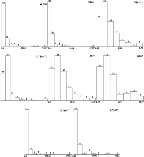
Table 1. Statistical characteristics of used data.

Variable	Mean	Minimum	Maximum	Standard deviation	Coefficient of variation	Skewness
W (m)	60.021	1.400	711.200	91.753	1.529	4.582
H (m)	1.550	0.140	19.940	2.131	1.375	5.243
U (ms^−1)	0.492	0.029	1.730	0.339	0.689	1.474
U* (ms^−1)	0.089	0.002	0.553	0.081	0.910	3.760
W/H	43.452	2.200	156.500	29.719	0.684	1.472
U/U*	6.954	0.770	20.770	4.651	0.669	1.186
K (m^2s^−1)	84.228	0.200	1486.500	180.816	2.147	4.777
K/(HU*)	785.110	3.080	7692.000	1119.676	1.426	3.336

Empirical models

Six empirical models used for estimation of the LDC in rivers are presented in Table 2. These empirical models may only be applicable within a range of specific flow and geometry, and may not provide appropriate results for other ranges.

Table 2. Empirical models for estimation of longitudinal dispersion coefficient (LDC) values.

Method	Equation	Notation
Fischer (1979)	$\frac{K}{H{U}_{\ast }}=0.011{\left(\frac{W}{H}\right)}^2{\left(\frac{U}{U_{\ast }}\right)}^2$	F
Seo and Cheong (1998)	$\frac{K}{H{U}_{\ast }}=5.915{\left(\frac{W}{H}\right)}^{0.62}{\left(\frac{U}{U_{\ast }}\right)}^{1.428}$	S-C
Kashefipour and Falconer (2002)	$\frac{K}{H{U}_{\ast }}=10.612{\left(\frac{U}{U_{\ast }}\right)}^2$	K-F
Sahay and Dutta (2009)	$\frac{K}{H{U}_{\ast }}=2{\left(\frac{W}{H}\right)}^{0.96}{\left(\frac{U}{U_{\ast }}\right)}^{1.25}$	S-D
Wang and Huai (2016)	$\frac{K}{H{U}_{\ast }}=17.648{\left(\frac{W}{H}\right)}^{0.3619}{\left(\frac{U}{U_{\ast }}\right)}^{1.16}$	W-H
Li, Liu, and Yin (2013)	$\frac{K}{H{U}_{\ast }}=2.828{\left(\frac{W}{H}\right)}^{3.7613}{\left(\frac{U}{U_{\ast }}\right)}^{1.4713}$	L

Machine learning models

M5 model tree (M5P)

The M5P algorithm, first introduced by Quinlan (1992), is an extended version of the M5 algorithm. Model trees can consider a set of data with a large number of features and sizes, and can work with a high degree of efficiency. The M5P algorithm contains four stages. The first stage is building a tree by dividing the input space into numerous subspaces. The variation in intra-space from root to node is lessened by using some attributes and division criteria. To measure the subspace variability, values of the standard deviation for each node are utilized. By using the standard deviation reduction (SDR) factor, the tree is built. This method remarkably reduces the expected errors in the node using the following equation (Behnood, Behnood, Gharehveran, & Alyamac, 2017): (2) $\text{SDR}=sd(T)-\sum _i\frac{|T_i|}{|T|}\times sd(T_i)$(2) where $sd$ denotes the standard deviation, T is a set of examples which reach the node, and $T_i$ is the outcomes of the node division pursuant to the attributes (Wang & Witten, 1997).

In the second step, the linear regression model is advanced in each of the subspaces for each node. Then, the pruning method is used to overcome the problem of overtraining, which happens when the correspondent SDR value of the linear model becomes lower than the predetermined error. The adjacent linear model can show severe disturbances in the results of pruning. This can mostly happen for models that are constructed from a small amount of training data, but can be balanced by smoothing in the last step. In the smoothing procedure, to create the last model of the leaf, all models from the leaf to the root are combined.

Support vector regression (SVR)

SVR evolved from SVMs, which were created by Vapnik (1995, 1998), and has been used in many hydrological applications (Choubin et al., 2019). This approach is a data-based method and it deals with the predicted problems and the structural risk minimization principle (Pai & Hong, 2007). Achieving a regression model with suitable predictive performance is the main goal of SVR. Variables in the SVR model comprise $(x_i,y_i{)}_{i=1}^N$, in which $x_i$ is the input parameter, $y_i$ is the output parameter and the total number of data is represented by N. The SVR is expressed as (Kalteh, 2013): (3) $f(x)=w\phi (x)+b$(3) where w is a weight vector, b is a threshold value, and $\phi (x)$ is a nonlinear mapping variable. Input patterns are designed in a large space; therefore, in the mapped space the model can be linearly regressed. In the SVR model, the optimal amounts of w and b are computed by the following formula: (4) $min\left\{\frac{1}{2}{||w||}^2+C\sum _{I=1}^n|y_t-f(x_t)|\right\}$(4) where C is the penalty parameter and n is the sample size.

Gaussian process regression (GPR)

GPR is defined as a set of random variables in which each variable has a common Gaussian distribution. To represent the relationship between inputs (x) and outputs (y), the f function should be defined and modeled for each possible entry. To achieve a model between x and y, a GPR model is constructed as the regression function and the noise term $(\epsilon \sim N(0,{\sigma }_n^2))$ is used in this function: (5) $y=f(x)+\epsilon$(5) where ${\sigma }_n$ is the standard deviation of the noise.

This can be completely determined by a mean $m(x)$ and a covariance $k(x,x^{\mathrm{\prime }})$: (6) $f(x)\sim GP(m(x),k(x,x^{\mathrm{\prime }}))$(6) where $m(x)=0$ is assumed to facilitate the computation and there are different choices for k. The covariance function, which is known as the kernel function, is a linear separator and is used to obtain the connection between the input and output of the model. If points are moved to higher spaces, their internal multiplication (k) will be changed too.

Selecting a suitable kernel function based on assumptions such as smoothness and possible patterns in the data is highly significant. The kernel functions used in this study are the polynomial kernel, the normalized poly kernel, the radial basis function or Gaussian kernel (RBF) and the Pearson universal kernel. In this section, the GPR modeling method has been introduced briefly; a more detailed explanation is given in Rasmussen and Williams (2006).

Random forest (RF)

RF is a series of complex relationships that are able to consider the interaction between predictors and responses without any relationships between them by including decision trees (Breiman, 2001). Each of the component trees forms an RF using available data. For each tree, a subset of predictions is chosen with the same chance. By combining and averaging the single predictions of all compounding trees, the predictive output is achieved. The RF algorithm consists of two random levels in each tree. The first step is bagging and the second is selection of the features randomly; studies have indicated that the performance of this model is superior to other models (Archer & Kimes, 2008; Woznicki, Baynes, Panlasigui, Mehaffey, & Neale, 2019). RF, without any assumptions about independent or dependent variables, explains both linear and nonlinear relationships.

Performance criteria

To statistically examine the performance of the models created in the current study, the correlation coefficient (CC), root mean squared error (RMSE) and mean absolute error (MAE) were used. The mathematical representations are cited as follows (Kargar, Sadegh Safari, Mohammadi, & Samadianfard, 2019; Samadianfard et al., 2019a): (7) $\begin{array}{rl}\text{CC}& =\frac{\left({\sum }_{i=1}^N{O}_i{P}_i-\frac{1}{N}{\sum }_{i=1}^N{O}_i{\sum }_{i=1}^N{P}_i\right)}{\begin{array}{c}\left({\sum }_{i=1}^N{O}_i^2-\frac{1}{N}{\left({\sum }_{i=1}^N{O}_i\right)}^2\right)\\ \left({\sum }_{i=1}^N{P}_i^2-\frac{1}{N}{\left({\sum }_{i=1}^N{P}_i\right)}^2\right)\end{array}}\end{array}$(7) (8) $\begin{array}{rl}\text{RMSE}& =\sqrt{\frac{1}{N}\sum _{i=1}^N{(P_i-O_i)}^2}\end{array}$(8) (9) $\begin{array}{rl}\text{MAE}& =\frac{1}{N}\sum _{i=1}^N(|P_i-O_i|)\end{array}$(9) where $O_i$ and $P_i$ are the measured and estimated value of the dispersion coefficient, $\overline{O}$ is the mean of measured $O$, and N represents the number of data.

In addition, Taylor diagrams (Taylor, 2001) were used to check the precision of the implemented models and empirical models for LDC estimation in natural rivers. It is notable that in these diagrams, measured and some corresponding statistical parameters are presented simultaneously. Moreover, different points on a polar plot are used in Taylor diagrams to investigate the differences between measured and estimated values. The CC and normalized standard deviation are specified by the azimuth angle and radial distances from the base point, respectively (Taylor, 2001).

Results and discussion

The capabilities of machine learning and data-driven algorithms, such as GPR, SVR, M5P and RF, in estimating LDC values in different streams were compared with the potential of common empirical models. For this purpose, the hydraulic parameters of several streams in different geographic locations, including channel width, depth of water, mean velocity, shear velocity and LDC, were gathered. In the current study, the whole data set including the hydraulic and geometric properties of 147 streams was randomly partitioned into training (67%) and testing data (33%), and the early stopping method (Graf, Zhu, & Sivakumar, 2019; Piotrowski & Napiorkowski, 2013) was performed to avoid overfitting. In other words, $\frac{W}{H}$ and $\frac{U}{U_{\ast }}$ were used for estimating LDC values. It should be noted that four kernel functions, namely polynomial, normalized polynomial, Pearson VII function-based and RBF, were investigated for the GPR (GPR-1, GPR-2, GPR-3, GPR-4) and SVR (SVR-1, SVR-2, SVR-3, SVR-4) models. The results of statistical parameters, including CC, RMSE and MAE, in LDC estimation for the considered models and common empirical models are displayed in Tables 3 and 4. It is obvious from Table 3 that among the GPR models, GPR-3, with CC of 0.679, RMSE of 590.2 and MAE of 460.9, had the best performance. Moreover, SVR-3, with CC of 0.788, RMSE of 460.8 and MAE of 321.4, estimated LDC values with lower errors than the other SVR models. It is notable that Pearson VII function-based GPR and SVR models (GPR-3 and ?>SVR-3) were more accurate than the other GPR and SVR models. In other words, the Pearson VII function-based kernel had more applicability in LDC estimation than the other mentioned kernel functions. Furthermore, it can be seen from Table 3 that M5P, with CC of 0.823, RMSE of 454.9 and MAE of 380.9, had precise prediction between machine learning and data-driven algorithms. Unlike the GPR, SVR and M5P models, RF, with CC of 0.482, RMSE of 858.4 and MAE of 576.0, and MLR, with CC of 0.605, RMSE of 617.4 and MAE of 452.6, had unacceptable accuracies and they are not recommended for LDC estimation. In addition, among the considered empirical models (Table 4), Sahay and Dutta (S-D), with CC of 0.795, RMSE of 460.7 and MAE of 306.1, had high precision in comparison with the other empirical models. In other words, errors generated by the S-D model are lower only than GPR-3, RF and MLR. This implies that SVR-3 and M5P are able to attain more accurate performance than the empirical models. From the statistical metrics presented in Tables 3 and 4, it can be concluded that the accuracy of M5P far exceeds the mentioned models and empirical models. In terms of the practical value of the M5P model, the resulting explicit formulations can provide a powerful and easy tool for accurate estimation of LDC values.

Table 3. Performance of machine learning models based on different statistical parameters.

	Statistical parameters
	Train			Test
Method	CC	RMSE	MAE	CC	RMSE	MAE
GPR-1	0.110	1382.2	876.5	0.078	811.1	671.5
GPR-2	0.528	1322.7	977.6	0. 645	909.4	832.0
GPR-3	0.634	1111.7	658.2	0.679	590.2	460.9
GPR-4	0.495	1359.8	847.5	0.493	778.4	636.9
SVR-1	0.069	1473.4	716.5	0.089	706.4	389.4
SVR-2	0.500	1268.8	634.2	0.651	564.7	332.1
SVR-3	0.631	1139.5	513.0	0.788	460.8	321.4
SVR-4	0.526	1377.9	687.6	0.547	646.9	410.9
M5P	0.666	1042.0	616.7	0.823	454.9	380.9
RF	0.965	452.0	271.1	0.482	858.4	576.0
MLR	0.411	1266.9	737.0	0.605	617.4	452.6

Note: CC = correlation coefficient; RMSE = root mean squared error; MAE = mean absolute error; GPR = Gaussian process regression; SVR = support vector regression; M5P = M5 model tree; RF = random forest; MLR = multiple linear regression.

Table 4. Performance of empirical models based on different statistical parameters.

Method	Statistical parameters
	CC	RMSE	MAE
F	0.809	2167.9	826.9
S-C	0.734	574.7	374.5
K-F	0.411	808.9	503.6
S-D	0.795	460.7	306.1
W-H	0.643	554.6	363.9
L	0.768	524.4	353.1

Note: CC = correlation coefficient; RMSE = root mean squared error; MAE = mean absolute error; F = Fischer; S-C = Seo and Cheong; K-F = Kashefipour and Falconer; S-D = Sahay and Dutta; W-H = Wang and Huai; L = Li, Liu, and Yin.

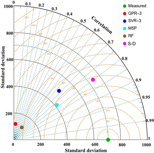
Scatterplots of the observed values of LDC and the corresponding values estimated by the studied methods and empirical models are shown in Figure 2. It is clear from Figure 2 that the estimates of M5P are less scattered across the bisection line. So, the estimates of M5P are much closer to the bisection line than those of the data-driven algorithms and empirical models. Figure 3 presents the measured and estimated values of LDC in the testing phase and Figure 4 illustrates the boxplots of the models. In accordance with the concluding remarks on the scatterplots and boxplots, it is obvious that the estimates of M5P are in better agreement with the measured LDC values. Additional evaluation of measured and estimated LDC values by GPR-3, SVR-3, M5P, RF and S-D was carried out and Figure 5 presents the obtained results. Figure 5 is an instrumental tool in understanding the different potential of the studied models. In the Taylor diagram, an accurate model is marked by the reference point with a correlation coefficient of 1 and the same amplitude of variation as the observations. According to the lower distance from the measured point (the green point in Figure 5) to the correspondent point of the M5P (the cyan point), the estimates of M5P were more accurate than the results of the other models. In other words, the lower distance of the M5P correspondent point to the observed point clearly indicates the high potential and capacities of M5P for providing accurate predictions of the LDC.

Figure 2. Scatterplots of measured and estimated dispersion coefficient. GPR = Gaussian process regression; SVR = support vector regression; M5P = M5 model tree; RF = random forest; MLR = multiple linear regression; F = Fischer; S-C = Seo and Cheong; K-F = Kashefipour and Falconer; S-D = Sahay and Dutta; W-H = Wang and Huai; L = Li, Liu, and Yin.

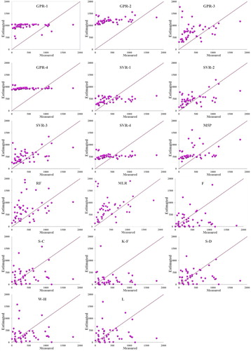
Figure 3. Series plots of measured and estimated dispersion coefficient values. GPR = Gaussian process regression; SVR = support vector regression; M5P = M5 model tree; RF = random forest; MLR = multiple linear regression; F = Fischer; S-C = Seo and Cheong; K-F = Kashefipour and Falconer; S-D = Sahay and Dutta; W-H = Wang and Huai; L = Li, Liu, and Yin.

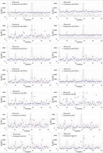
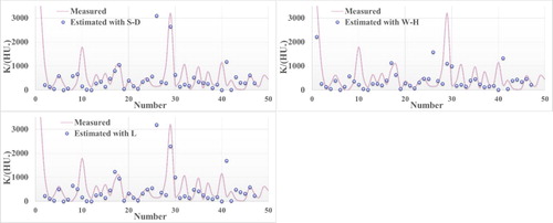
Figure 4. Boxplots of measured and estimated dispersion coefficient values. GPR = Gaussian process regression; SVR = support vector regression; M5P = M5 model tree; RF = random forest; MLR = multiple linear regression; F = Fischer; S-C = Seo and Cheong; K-F = Kashefipour and Falconer; S-D = Sahay and Dutta; W-H = Wang and Huai; L = Li, Liu, and Yin.

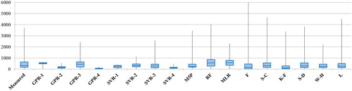
Figure 5. Taylor diagram of estimated dispersion coefficient values. GPR = Gaussian process regression; SVR = support vector regression; M5P = M5 model tree; RF = random forest; S-D = Sahay and Dutta.

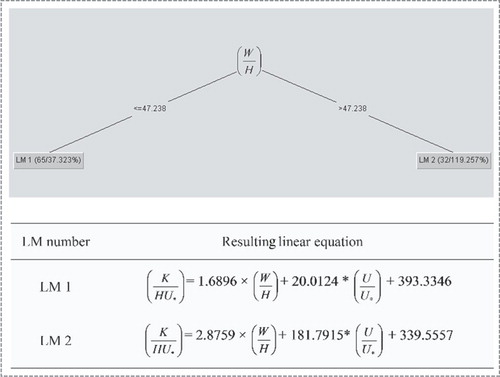
The tree structure resulting from the M5P model, as the most accurate model, is displayed in Figure 6. This illustrated tree model is based on the characteristics of used streams, and two linear equations are applied for LDC estimation, while the other data-driven models studied do not have such accuracy and capability. Being able to obtain explicit formulae for the LDC in M5P is another advantage of this model. Explicit formulae make it possible to evaluate the relative importance of the effective dimensionless parameters on the LDC. The formulae indicate that the parameter U/U_* has a great effect on LDC estimation, and the effect of this dimensionless parameter will be more significant in wide rivers.

Figure 6. M5P-obtained tree with two different linear models (LM).

Comparison of the obtained results with the ANN results of Tayfour and Singh (2005) showed that although the accuracy of M5P (with RMSE of 454.9), as the best studied model, is lower than the ANN developed by Tayfour and Singh (2005) (with RMSE of 193.0), the practical mathematical formulations of M5P mean that is highly applicable in LDC estimation.

Sensitivity analysis

To investigate the influence of input parameters on LDC estimation, CC, RMSE and MAE evaluation criteria were used for different input variables. For this purpose, the M5P was selected for sensitivity analysis, as this was the most accurate model in LDC estimation (Table 5). Each model confirmed the extent to which the eliminated variable would affect the model accuracy. It is clear from Table 5 that the precision of the M5P model decreased if either the W/H or U/U_* input parameter was removed from the modeling. Furthermore, it can be seen that W/H has the most significant effect in increasing the prediction accuracy. In other words, eliminating W/H caused a sharp increase in the RMSE value.

Table 5. Effect of removing input variables on the M5P model accuracy for longitudinal dispersion coefficient (LDC) estimation.

		Statistical parameters
Model	Input parameters	CC	RMSE	MAE
1	All	0.823	454.9	380.9
2	Remove W/H	0.405	766.6	572.3
3	Remove U/U*	0.518	676.1	513.8

Note: CC = correlation coefficient; RMSE = root mean squared error; MAE = mean absolute error.

Conclusion

In this study, various machine learning algorithms, including GPR, SVR, M5P and RF, were used to estimate LDC values in natural streams and rivers. LDC values can be estimated using flow variables and geometric characteristics of the channel. So, in the current research, $\frac{W}{H}$ and $\frac{U}{U_{\ast }}$ were considered as input parameters and $\frac{K}{U_{\ast }H}$ as an output parameter. The performances of the models were evaluated based on error measures of CC, RMSE, MAE and the Taylor diagram. The results indicated that although GPR-3 and SVR-3 using the Pearson VII function-based kernel and M5P showed satisfactory performance, M5P provided the most accurate estimations of LDC. Furthermore, among six common empirical models that were implemented in the current study, the S-D model gave the best result. In conclusion, the developed M5P model outperformed others in terms of accuracy and it is recommended for LDC estimation. In addition, the importance of the dimensionless parameter U/U* on LDC estimation, especially for wide rivers, was reported based on the findings of the current research. Finally, other hybrid machine learning algorithms could be implemented to test their capabilities in order to investigate possible improvements in the accuracy of LDC estimations.

Acknowledgments

We acknowledge the financial support for this work by the Hungarian State and the European Union under the EFOP-3.6.1-16-2016-00010 project. Furthermore, we acknowledge the support of the German Research Foundation (DFG) and the Bauhaus-Universität Weimar within the Open-Access Publishing Programme.

Disclosure statement

No potential conflict of interest was reported by the authors.

ORCID

Shahaboddin Shamshirband http://orcid.org/0000-0002-6605-498X

Amir Mosavi http://orcid.org/0000-0003-4842-0613

References

- Alizadeh, M. J., Jafari Nodoushan, E., Kalarestaghi, N., & Chau, K. W. (2017). Toward multi-day-ahead forecasting of suspended sediment concentration using ensemble models. Environmental Science and Pollution Research, 24(36), 28017–28025. doi: 10.1007/s11356-017-0405-4
- Archer, K. J., & Kimes, R. V. (2008). Empirical characterization of random forest variable importance measures. Computational Statistics & Data Analysis, 52(4), 2249–2260. doi: 10.1016/j.csda.2007.08.015
- Azamathulla, H. M., & Ghani, A. A. (2011). Genetic programming for predicting longitudinal dispersion coefficients in streams. Water Resources Management, 25(6), 1537–1544. doi: 10.1007/s11269-010-9759-9
- Behnood, A., Behnood, V., Gharehveran, M. M., & Alyamac, K. E. (2017). Prediction of the compressive strength of normal and high-performance concretes using M5P model tree algorithm. Construction and Building Materials, 142, 199–207. doi: 10.1016/j.conbuildmat.2017.03.061
- Bencala, K. E., & Walters, R. A. (1983). Simulation of solute transport in a mountain pool-and-riffle stream: A transient storage model. Water Resource Research, 19(3), 718–724. doi: 10.1029/WR019i003p00718
- Breiman, L. (2001). Random forests. Machine Learning, 1(5), 32–45.
- Chau, K. W. (2000). Transverse mixing coefficient measurements in an open rectangular channel. Advances in Environmental Research, 4(4), 287–294. doi: 10.1016/S1093-0191(00)00028-9
- Chen, X. U., & Chau, K. W. (2016). A hybrid double feedforward neural network for suspended sediment load estimation. Water Resources Management, 30(7), 2179–2194. doi: 10.1007/s11269-016-1281-2
- Choubin, B., Moradi, E., Golshan, M., Adamowski, J., Sajedi-Hosseini, F., & Mosavi, A. (2019). An ensemble prediction of flood susceptibility using multivariate discriminant analysis, classification and regression trees, and support vector machines. Science of the Total Environment, 651, 2087–2096. doi: 10.1016/j.scitotenv.2018.10.064
- Dehghani, M., Riahi-Madvar, H., Hooshyaripor, F., Mosavi, A., Shamshirband, S., Zavadskas, E. K., & Chau, K. (2019). Prediction of hydropower generation using grey wolf optimization adaptive neuro-fuzzy inference system. Energies, 12(12), 289. doi: 10.3390/en12020289
- Esmaeilzadeh, B., Sattari, M. T., & Samadianfard, S. (2017). Performance evaluation of ANNs and an M5 model tree in Sattarkhan Reservoir inflow prediction. ISH Journal of Hydraulic Engineering, 23(3), 283–292. doi: 10.1080/09715010.2017.1308277
- Etemad-Shahidi, A., & Taghipour, M. (2012). Predicting longitudinal dispersion coefficient in natural streams using M5’ model tree. Journal of Hydraulic Engineering, 138(6), 542–554. doi: 10.1061/(ASCE)HY.1943-7900.0000550
- Fischer, H. B. (1968). Dispersion predictions in natural streams. Journal of the Sanitary Engineering Division, ASCE, 94(5), 927–943.
- Fischer, H. B. (1979). Mixing in inland and coastal waters. San Diego, CA: Academic Press.
- Graf, B. (1995). Observed and predicted velocity and longitudinal dispersion at steady and unsteady flow, Colorado River, Glen Canyon Dam to Lake Mead. Water Resources Bulletin, 31(2), 265–281. doi: 10.1111/j.1752-1688.1995.tb03379.x
- Graf, R., Zhu, S., & Sivakumar, B. (2019). Forecasting river water temperature time series using a wavelet–neural network hybrid modelling approach. Journal of Hydrology, 578, 124115. doi: 10.1016/j.jhydrol.2019.124115
- Houichi, L., Dechemi, N., Heddam, S., & Achour, B. (2012). An evaluation of ANN methods for estimating the lengths of hydraulic jumps in U-shaped channel. Journal of Hydroinformatics, 15(1), 147–154. doi: 10.2166/hydro.2012.138
- Jirka, G. H. (2004). Mixing and dispersion in rivers. London: Taylor and Francis, pp. 13–27.
- Julínek, T., & Říha, J. (2017). Longitudinal dispersion in an open channel determined from a tracer study. Environmental Earth Sciences, 76(17), 592. doi: 10.1007/s12665-017-6913-1
- Kalteh, A. M. (2013). Monthly river flow forecasting using artificial neural network and support vector regression models coupled with wavelet transform. Computers & Geosciences, 54, 1–8. doi: 10.1016/j.cageo.2012.11.015
- Kargar, K., Sadegh Safari, M. J., Mohammadi, M., & Samadianfard, S. (2019). Sediment transport modeling in open channels using neuro-fuzzy and gene expression programming techniques. Water Science and Technology, 79(12), 2318–2327. doi: 10.2166/wst.2019.229
- Kashefipour, S. M., & Falconer, R. A. (2002). Longitudinal dispersion coefficients in natural channels. Water Resource, 36, 1596–1608.
- Li, X., Liu, H., & Yin, M. (2013). Differential evolution for prediction of longitudinal dispersion coefficients in natural streams. Water Resources Management, 27(15), 5245–5260.
- McQuivey, R. S., & Keefer, T. N. (1974). Simple method for predicting dispersion in streams. Journal of Environmental Engineering, 100(4), 997–1011.
- Mosavi, A., Ozturk, P., & Chau, K. W. (2018). Flood prediction using machine learning models: Literature review. Water, 10(11), 1536. doi: 10.3390/w10111536
- Noori, R., Deng, Z., Kiaghadi, A., & Kachoosangi, F. T. (2015). How reliable are ANN, ANFIS, and SVM techniques for predicting longitudinal dispersion coefficient in natural rivers? Journal of Hydraulic Engineering, 142(1), 04015039. doi: 10.1061/(ASCE)HY.1943-7900.0001062
- Nordin, C. F., & Sabol, G. V. (1974). Empirical data on longitudinal dispersion in rivers. Washington, DC: US Geological Survey Water Resource Investigation 20-74.
- Olyaie, E., Banejad, H., Chau, K. W., & Melesse, A. M. (2015). A comparison of various artificial intelligence approaches performance for estimating suspended sediment load of river systems: A case study in United States. Environmental Monitoring and Assessment, 187, 189. doi: 10.1007/s10661-015-4381-1
- Pai, P., & Hong, W. (2007). A recurrent support vector regression model in rainfall forecasting. Hydrological Process, 21, 819–827. doi: 10.1002/hyp.6323
- Piotrowski, A. P., & Napiorkowski, J. J. (2013). A comparison of methods to avoid overfitting in neural networks training in the case of catchment runoff modeling. Journal of Hydrology, 476, 97–111. doi: 10.1016/j.jhydrol.2012.10.019
- Pourabadei, M., & Kashefipour, S. M. (2007). Investigation of flow parameters on dispersion coefficient of pollutants in canal. In Proceedings of the 6th International symposium river engineering, October (pp. 16–18).
- Qasem, S. N., Samadianfard, S., Kheshtgar, S., Jarhan, S., Kisi, O., Shamshirband, S., & Chau, K. W. (2019a). Modeling monthly pan evaporation using wavelet support vector regression and wavelet artificial neural networks in arid and humid climates. Engineering Applications of Computational Fluid Mechanics, 13(1), 177–187. doi: 10.1080/19942060.2018.1564702
- Qasem, S. N., Samadianfard, S., Nahand, H. S., Mosavi, A., Shamshirband, S., & Chau, K. W. (2019b). Estimating daily dew point temperature using machine learning algorithms. Water, 11(3), 582. doi: 10.3390/w11030582
- Quinlan, J. R. (1992). Learning with continuous classes. In Proceedings of the Australian joint conference on artificial Intelligence, world scientific (pp. 343–348). Singapore.
- Rasmussen, C. E., & Williams, C. K. I. (2006). Gaussian processes for machine learning. Cambridge, MA: MIT Press.
- Riahi-Madvar, H., Ayyoubzadeh, S. A., Khadangi, E., & Ebadzadeh, M. M. (2009). An expert system for predicting longitudinal dispersion coefficient in natural streams by using ANFIS. Expert Systems with Applications, 36(4), 8589–8596. doi: 10.1016/j.eswa.2008.10.043
- Rutherford, J. C. (1994). River mixing. Chichester, UK: Wiley, p. 347.
- Sahay, R. R. (2011). Prediction of longitudinal dispersion coefficients in natural rivers using artificial neural network. Environmental Fluid Mechanics, 11(3), 247–261. doi: 10.1007/s10652-010-9175-y
- Sahay, R. R., & Dutta, S. (2009). Prediction of longitudinal dispersion coefficients in natural rivers using genetic algorithm. Hydrology Research, 40(6), 544–552. doi: 10.2166/nh.2009.014
- Samadianfard, S., Delirhasannia, R., Torabi Azad, M., Samadianfard, S., & Jeihouni, M. (2016). Intelligent analysis of global warming effects on sea surface temperature in Hormuzgan Coast, Persian Gulf. International Journal of Global Warming, 9(4), 452–466. doi: 10.1504/IJGW.2016.076331
- Samadianfard, S., Ghorbani, M. A., & Mohammadi, B. (2018). Forecasting soil temperature at multiple-depth with a hybrid artificial neural network model coupled-hybrid firefly optimizer algorithm. Information Processing in Agriculture, 5(4), 465–476. doi: 10.1016/j.inpa.2018.06.005
- Samadianfard, S., Jarhan, S., Salwana, E., Mosavi, A., Shamshirband, S., & Akib, S. (2019a). Support vector regression integrated with fruit fly optimization algorithm for river flow forecasting in Lake Urmia Basin. Water, 11(9), 1934. doi: 10.3390/w11091934
- Samadianfard, S., Majnooni-Heris, A., Qasem, S. N., Kisi, O., Shamshirband, S., & Chau, K. W. (2019b). Daily global solar radiation modeling using data-driven techniques and empirical equations in a semi-arid climate. Engineering Applications of Computational Fluid Mechanics, 13(1), 142–157. doi: 10.1080/19942060.2018.1560364
- Seo, I. W., & Cheong, T. S. (1998). Predicting longitudinal dispersion coefficient in natural streams. Journal of Hydraulic Engineering, 124(1), 25–32. doi: 10.1061/(ASCE)0733-9429(1998)124:1(25)
- Tayfour, G., & Singh, V. P. (2005). Predicting longitudinal dispersion coefficient in natural streams by artificial neural network. Journal of Hydraulic Engineering, 131(11), 991–1000. doi: 10.1061/(ASCE)0733-9429(2005)131:11(991)
- Taylor, G. (1954). The dispersion of matter in turbulent flow through a pipe. Proceedings of the Royal Society of London A: Mathematical, Physical and Engineering Sciences, 223(1155), 446–468. doi: 10.1098/rspa.1954.0130
- Taylor, K. E. (2001). Summarizing multiple aspects of model performance in a single diagram. Journal of Geophysical Research: Atmospheres, 106, 7183–7192. doi: 10.1029/2000JD900719
- Vapnik, V. (1995). The nature of statistical learning theory. New York: Springer, p. 187.
- Vapnik, V. (1998). Statistical learning theory. New York: John Wiley & Sons, p. 740.
- Wang, Y., & Huai, W. (2016). Estimating the longitudinal dispersion coefficient in straight natural rivers. Journal of Hydraulic Engineering, 142(11).
- Wang, Y., Huai, W., & Wang, W. (2017). Physically sound formula for longitudinal dispersion coefficients of natural rivers. Journal of Hydrology, 544, 511–523. doi: 10.1016/j.jhydrol.2016.11.058
- Wang, Y., & Witten, I. H. (1997). Induction of model trees for predicting continuous classes. In Proceedings European conference on machine learning, Prague, Czechoslovakia.
- Woznicki, S. A., Baynes, J., Panlasigui, S., Mehaffey, M., & Neale, N. (2019). Development of a spatially complete floodplain map of the conterminous United States using random forest. Science of the Total Environment, 647, 942–953. doi: 10.1016/j.scitotenv.2018.07.353
- Zeng, Y., & Huai, W. (2014). Estimation of longitudinal dispersion coefficient in rivers. Journal of Hydro-environment Research, 8(1), 2–8. doi: 10.1016/j.jher.2013.02.005
- Zhu, S., Heddam, S., Nyarko, E. K., Hadzima-Nyarko, M., Piccolroaz, S., & Wu, S. (2019). Modeling daily water temperature for rivers: Comparison between adaptive neuro-fuzzy inference systems and artificial neural networks models. Environmental Science and Pollution Research, 26(1), 402–420. doi: 10.1007/s11356-018-3650-2