Modeling monthly pan evaporation process over the Indian central Himalayas: application of multiple learning artificial intelligence model

Abstract

The potential of several predictive models including multiple model-artificial neural network (MM-ANN), multivariate adaptive regression spline (MARS), support vector machine (SVM), multi-gene genetic programming (MGGP), and ‘M5Tree’ were assessed to simulate the pan evaporation in monthly scale (EP_m) at two stations (e.g. Ranichauri and Pantnagar) in India. Monthly climatological information were used for simulating the pan evaporation. The utmost effective input-variables for the MM-ANN, MGGP, MARS, SVM, and M5Tree were determined using the Gamma test (GT). The predictive models were compared to each other using several statistical criteria (e.g. mean absolute percentage error (MAPE), Willmott's Index of agreement (WI), root mean squared error (RMSE), Nash-Sutcliffe efficiency (NSE), and Legate and McCabe’s Index (LM)) and visual inspection. The results showed that the MM-ANN-1 and MGGP-1 models (NSE, WI, LM, RMSE, MAPE are 0.954, 0.988, 0.801, 0.536 mm/month, 9.988% at Pantnagar station, and 0.911, 0.975, 0.724, and 0.364 mm/month, 12.297% at Ranichauri station, respectively) with input variables equal to six were more successful than the other techniques during testing period to simulate the monthly pan evaporation at both Ranichauri and Pantnagar stations. Thus, the results of proposed MM-ANN-1 and MGGP-1 models will help to the local stakeholders in terms of water resources management.

KEYWORDS:

• Pan evaporation
• multiple model strategy
• gamma test
• Indian central Himalayas
• meteorological variables

1. Introduction

Evaporation plays the main role in environmental studies and water resources management. Therefore, the precise simulation of EP_m is necessary for hydrological simulating, river flow forecasting, forestry, lake-ecosystems, agronomy and irrigation sciences (Burt, Mutziger, Allen, & Howell, 2005). The most effective meteorological factors on evaporation rate are relative humidity, air temperature, vapor pressure deficit, atmospheric pressure, vapor pressure, wind speed, and sunshine hours (Yaseen et al., 2019). Evaporation is generally measured using two methods: (i) direct methods such as Class A pan-evaporimeter and (ii) indirect methods include empirical equations (Ghorbani, Deo, Yaseen, Kashani, & Mohammadi, 2017). Doorenbos and Pruitt (1977) said that the Class A pan-evaporimeter performance was affected by the turbidity of the water, watering of birds or other animals, human and instrumentation errors, and maintenance problems. Numerous studies reported the determination of the pan evaporation applying some empirical and semi-empirical formulations based on various meteorological information (Griffiths, 1966; Penman, 1948; Priestley & Taylor, 1972). However, there are limitations to the applications of these methods because of using different climatic factors. Therefore, alternative methods, which require less meteorological data are needed to predict the evaporation (Kisi, 2015; Kisi, Genc, Dinc, & Zounemat-Kermani, 2016).

AI models has shown promising progress on the evaporation estimation (Tao et al., 2018). Several versions of AI models are explored for pan evaporation simulation including; ANN based models, Fuzzy based models, support vector machine (SVM), evolutionary computing, data mining and complementary wavelet-AI models (Adnan, Malik, Kumar, Parmar, & Kisi, 2019; Guven & Kisi, 2013; Kisi & Heddam, 2019; Qasem et al., 2019; Qutbudin et al., 2019; Rezaie-Balf, Kisi, & Chua, 2019; Sebbar, Heddam, & Djemili, 2019; Yaseen, El-shafie, Jaafar, Afan, & Sayl, 2015). Tabari, Talaee, and Abghari (2012) predicted daily pan-evaporation using CANFIS and MLPNN techniques in Iran. The research findings demonstrated that the MLPNN model provided a better accuracy than the CANFIS model. Kisi (2015) used least square SVM (LSSVM), M5Tree, and MARS for estimating pan evaporation in Turkey. They found that the MARS provided a significant superiority compared to other models. Deo, Samui, and Kim (2016) developed the ELM, MARS, and relevance vector machine (RVM) to predict evaporative using maximum and minimum temperatures, atmospheric vapor pressure, precipitation and solar radiation in Australia. The results indicated that the RVM model has high ability compared to the other techniques. Malik and Kumar (2015) hired the CANFIS, MLR, and ANN models for predicting the pan evaporation over different stations in India and the ANN models are more successful compared to other ones. Keshtegar, Piri, and Kisi (2016) used M5Tree, conjugate gradient (CG), and ANFIS models to simulate of evaporation. Results produced that the CG model is more satisfactory than the M5Tree and ANFIS techniques. Wang, Kisi, Zounemat-Kermani, and Li (2017) estimated pan evaporation using the FG, ANFIS-GP, and M5Tree models in China. Results proved the high ability of the FG model in pan evaporation estimation. Wang, Kisi, Hu, et al. (2017) predicted pan evaporation using MLPNN, GRNN, ANFIS with grid partition (ANFIS-GP), MARS, MLR, FG, LSSVM, and SS models in China. The results showed that the AI models provided the most accuracy than the SS and MLR techniques. Wang, Niu, Kisi, Li, and Yu (2017) evaluated the LSSVR, MARS, MLR, FG, and M5Tree models for simulating EP_m in daily scale in China. Results demonstrated that the LSSVR and FG models show the highest accuracy to the other applied models in pan evaporation estimation.

Furthermore, the current research the correlated input variables are identified using a nonlinear method called Gama Test (GT). In recent decade, various researches about applying Gamma test have been done in numerous cases (Malik & Kumar, 2018; Remesan, Shamim, & Han, 2008; Singh, Malik, Kumar, & Kisi, 2018). Moghaddamnia, Ghafari Gousheh, Piri, Amin, and Han (2009) simulated evaporation using the ANN and ANFIS models while applying GT to select suitable input variables in different area of Iran. Results showed the ANFIS and ANN models have high capability in the estimation of EP_m values. Goyal, Bharti, Quilty, Adamowski, and Pandey (2014) identified suitable input variables using GT for FL, ANN, ANFIS, and least square-SVM techniques to estimate EP_m in daily scale in India, and the SS and Hargreaves-Samani (HGS) equations were compared with the results obtained by AI models. The study showed the superior accuracy of the SCT over SS and HGS techniques. Malik, Kumar, and Kisi (2018) simulated daily EP_m using RBNN, MLR, Griffiths, Stephens-Stewart, Priestley-Taylor, Christiansen, Penman, SOMNN, and Jensen-Burman-Allen models in India. The input combinations of MLR, RBNN, and SOMNN were determined using the GT. The results of the research indicated that the most accuracy was observed in the RBNN model.

The current research is conducted to accomplish the following aims:

1. An appropriate input combination is identified using GT before the construction of the proposed and comparable predictive models.

2. Potential of the proposed model is investigated using climate information of Ranichauri and Pantnagar stations located in Indian central Himalayas.

3. A comprehensive evaluation is performed on the obtained performance of the proposed predictive models.

2. Material and methods

2.1. Description of case study

The sources of the weather information used in this study are two stations (i.e. Ranichauri and Pantnagar) in India. The coordinates of the Pantnagar and Ranichauri stations are (79° 38′ 0′′ E, 29° 0′ 0′′ N) and (78° 24′ 35′′ E, 30° 18′ 40′′ N), respectively. These coordinates are depicted in Figure 1. The Pantnagar and Ranichauri stations are located at altitude of 243.8 and 2000 m above sea level, respectively. The recorded meteorological information was collected from the Crop Research Centres in Uttarakhand, India are the monthly minimum (T_min) and maximum temperatures (T_max), the wind speed (S_w), the hours of sunshine (H_ss), the monthly pan evaporation (EP_m), and the morning and afternoon relative humidity (RH₁ and RH₂). The EP_m in monthly scale were obtained from Crop Research Centre (CRC) observatory. Figure 2(a and b) depict the box–whisker plots of the meteorological information collected over 27 years at Pantnagar station (January 1990 to December 2016), and at Ranichauri station for over 13 years (January 2000 to December 2012), respectively. These plots provide information such as the minimum, quartile-wise, and maximum values of meteorological data. The collected data was partitioned into two different sets of varying strengths, (i) the training dataset, which was selected from January to December years 1990–2010 at the Pantnagar station, and years 2000–2009 at the Ranichauri station; and (ii) testing dataset, which was selected from January to December years 2011–2016 at the Pantnagar station and years 2010–2012 at the Ranichauri station. The correlation statistic between the predictive and target variables for both stations are presented in Table 1. This table shows that the input variables (i.e. RH₁, RH_2, S_w, T_min, T_max, and H_ss) have better cross-correlations (significant in statistics) with the output variable EP_m at 5% confidence level for Pantnagar station. Besides, the input variables (i.e. RH₁, H_ss, T_min, and T_max) have better cross-correlation (significant in statistics) with the output variable EP_m at 95% confidence level for Ranichauri station. It was also observed from Table 1, that there was no significant cross-correlation between T_min and H_ss variables for Pantnagar station, and T_min, S_w; T_min, H_ss; T_max, RH₁; T_max, RH_2; T_max, S_w; RH_2, EP_m; and S_w and EP_m variables for Ranichauri stations.

Figure 1. Location of the studied meteorological stations.

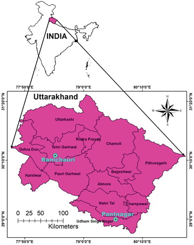
Figure 2. Box-Whisker plot of monthly meteorological data at (a) Pantnagar station, and (b) Ranichauri station.

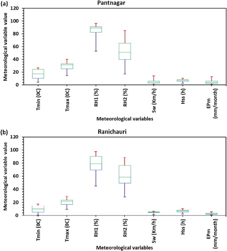
Table 1. Inter-correlation between climatic variables at Pantnagar and Ranichauri stations.

Variables	Tmin	Tmax	RH1	RH2	Sw	Hss	EPm
Pantnagar
Tmin	1.0
Tmax	0.8392*	1.0
RH1	−0.4024*	−0.7483*	1.0
RH2	0.2899*	−0.2468*	0.6552*	1.0
Sw	0.4864*	0.5258*	−0.5822*	−0.1625*	1.0
Hss	0.0251	0.4830*	−0.6238*	−0.7690*	0.1462*	1.0
EPm	0.6324*	0.8583*	−0.8947*	−0.4213*	0.6813*	0.5138*	1.0
Ranichauri
Tmin	1.0
Tmax	0.9110*	1.0
RH1	0.2745*	−0.0699	1.0
RH2	0.4502*	0.0951	0.9546*	1.0
Sw	−0.1348	−0.0534	−0.2983*	−0.3158*	1.0
Hss	−0.1104	0.2581*	−0.7854*	−0.8030*	0.3435*	1.0
EPm	0.7430*	0.8597*	−0.2811*	−0.1243	0.0675	0.3507*	1.0

*Statistically significant correlation at 5% level of significance.

2.2. Gamma test (GT)

Gamma test which includes continuous nonlinear models calculates the minimum standard error (SE) for a dataset. A data sample would be characterized as following formulas (Tsui, Jones, & De Oliveira, 2002); (1) $\left\{x_1\right(i),\dots ,x_m(i),y_i\}=\left\{\right(x_i,y_i)|1\le i\le M\}$(1) where, the x = ($x_1$, … , $x_m$) is the vector of inputs; $y_i$ is the target; M and m are the number patterns and inputs, respectively. The GT extracts the k^th (k = 1 … p) nearest neighbor lists (p is a user defined parameters) $x_{N\left[i,k\right]}$ (i = 1 … M) of the input vector ($x_i$). Finally, the GT calculates the following four statistics (Remesan, Shamim, Han, & Mathew, 2009): (2) ${\mathrm{\Delta }}_M\left(k\right)=\frac{1}{M}\sum _{i=1}^M|x_{N\left[i,k\right]}-x_i{|}^2\left(k=1\dots p\right)$(2) where, | … | indicates the Euclidean distance. Equation (3) indicates the gamma function of the output as (Moghaddamnia et al., 2009): (3) ${\gamma }_M\left(k\right)=\frac{1}{2M}\sum _{i=1}^M|y_{N\left[i,k\right]}-y_i{|}^2\left(k=1\dots p\right)$(3) where, $y_{N\left[i,k\right]}$ is the output of the k^th nearest neighbor of x_i. To calculate the gamma (Γ), a linear function is obtained using the p points {${\mathrm{\Delta }}_M\left(k\right),{\gamma }_M\left(k\right)$} as follows (Piri et al., 2009): (4) $y=A\delta +\mathrm{\Gamma }$(4) where, A = gradient, Γ = intercept ($\delta$ = 0), and y = output vector. Small values of the Γ (near to 0) shows that the input parameter has been selected more logically. The standard error (SE) of Γ is computed to measure the gamma value reliability. Small values of the SE shows that the gamma value is more reliable. V_ratio reveals the predictability of model, and defined as (Malik et al., 2018): (5) $V_{\text{ratio}}=\frac{\mathrm{\Gamma }}{{\sigma }^2\left(y\right)}$(5) where Γ is the gamma function and ${\sigma }^2\left(y\right)$ shows the output variance. The smaller V _ratio indicates the predictability of the model output.

It will be possible to create a high-quality mathematical model (e.g. MM-ANN, MARS, MGGP, SVM, and M5Tree) if the mentioned four factors i.e. A, SE, Γ, and V _ratio are small. In this research, the best predictive variables were picked using the obtained lowest values of Γ and V ratio (Malik, Kumar, Ghorbani, et al., 2019; Piri et al., 2009) for both stations.

2.3. Multiple model-artificial neural networks (MM-ANN)

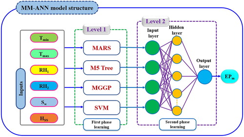
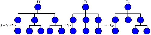
In this research, the multiple model-artificial neural networks (MM-ANN), which is a hybrid model was used as to simulate the evaporation process. This hybrid model includes two levels of modeling learning. Level 1 manages the primary learning process, and the main inputs (meteorological variables) and output (pan evaporation) variables are used for training the candidate AI models, this is in one land. On the other hand, the Level 2 modeling process is initiated based on the Level one result. In this manner, a kind of binary learning process of machine learning modeling strategy is initiated. The outputs of level 1 learning process are utilized as input attributes while the original output (i.e. pan evaporation) is used as outputs in Level 2 (See Figure 3). The established modeling strategy in the current research evidenced its potential in multiple hydrological engineering application such as soil cation exchange capacity, streamflow prediction, inflow detection (Ghorbani, Khatibi, Karimi, Yaseen, & Zounemat-Kermani, 2018; Kashani, Ghorbani, Shahabi, Naganna, & Diop, 2020; Khatibi, Ghorbani, Jani, & Servati, 2018; Khatibi, Ghorbani, & Pourhosseini, 2017). Yet, for the evaporation process to be investigated. This is due to the fact; the evaporation process is highly stochastic and non-linear characterized and thus such a binary ‘multiple model learning’ is needed here.

Figure 3. The structure of the MM-ANN model.

2.4. Multivariate adaptive regression spline (MARS)

The MARS model represents a linear model that can auto-simulate parametric interactions and nonlinearities (Friedman, 1991). This model has a backward and forward stepwise plan, where the plan that will ensure an over-trained and complex model after series of splits but with a lower accuracy is chosen at the forward stepwise plan (De Andrés, Lorca, de Cos Juez, & Sánchez-Lasheras, 2011). However, the previously chosen non-obligatory variables are removed at the backward stepwise plan. This function uses two functions (e.g. a knot – a value of a variable) that represents the meeting point within range of inputs to map X to Y (Adamowski, Chan, Prasher, & Sharda, 2012). Two functions [(x-t)₊ and (t-x)₊] are deployed in MARS. Here, ‘+’ represents only the positive as follows (Deo, Kisi, & Singh, 2017; Kisi, 2015): (6) $(x-t{)}_{+}=\left\{\begin{array}{c}x-t,\text{if }x>t\\ 0,\text{otherwise}\end{array}\right.$(6) (7) $(t-x{)}_{+}=\left\{\begin{array}{c}t-x,\text{if }x<t\\ 0,\text{otherwise}\end{array}\right.$(7)

The MARS formula is written as following equation: (8) $\hat{f}\left(x\right)=\sum _i^k{c}_i{B}_i\left(x\right)$(8) where c_i is the constant coefficients, and B_i(x) indicates a weighted sum of function. To run the MARS model, the Salford Predictive Modeler 8 software was utilized.

2.5. Multi-gene genetic programming (MGGP)

The MGGP is the advanced stage of classical genetic programming (GP), which improves the fitness of classical GP by linearly combining low depth GP trees (Searson, 2015). Several types of research about different genotype GP have been reported in various fields by (Danandeh Mehr & Nourani, 2017; Guven, 2009; Shoaib, Shamseldin, Melville, & Khan, 2015; Zorn & Shamseldin, 2015). Figure 4 represents the tree structure while the function is as follows (Danandeh Mehr, Kahya, & Olyaie, 2013): (9) $F\left(X_1,X_2\right)=\left(\right(3.5X_1÷Cos\left(X_2\right)+\text{exp}\left(Cos\left(X_1\right)\right)$(9) The major inputs of GP include (i) training/validation pattern; (ii) function for fitness (iii) leaves and inner nodes for identifying the structure; and (iv) the syntax tree formation parameters (Danandeh Mehr & Nourani, 2017). For simple problems, the arithmetic parameters including plus (+), minus (-), divide (÷), and multiply (x) have been used whereas for more complex problems, other operators including exp, cos, sin, and tan are applied (Searson, 2015). For example, a pseudo-linear MGGP chromosome predicts the predictand $\hat{\mathrm{y}}$ using several input variables as shown in Figure 5. The mathematical expression can be expressed as (Danandeh Mehr & Kahya, 2017; Danandeh Mehr, Kahya, & Yerdelen, 2014): (10) $\hat{y}=b_0+b_1{T}_1+b_2{T}_2,\dots \dots ,+b_G{T}_G$(10) where $\hat{y}$ is the estimated value; ${\text{T}}_{\text{i}}$ is the i^th gene output; ${\text{b}}_0$ is the noise; and ${\text{b}}_1$,${\text{b}}_2$, … ,${\text{b}}_{\text{G}}$ are the gene weights. The more detailed information about MGGP is given by (Danandeh Mehr & Kahya, 2017; Danandeh Mehr & Nourani, 2017).

Figure 4. GP tree structure of expression $\left(\right(3.5X_1÷\text{C}os\left(X_2\right)+\text{exp}\left(\text{C}os\left(X_1\right)\right)$.

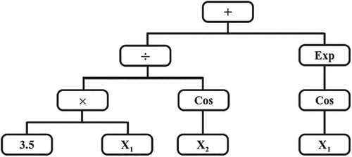
Figure 5. Multi-gene genetic programming (symbolic regression).

In this study MGGP framework topology was developed using 500 population size, 300 generations, mutation probability rate of 0.5, crossover probability rate of 0.4, reproduction probability rate of 0.1, 5 genes (trees), 4 depth of tree, and function set (divide, minus, plus, sin, cos, sqrt. log, exp.) in MATLAB software.

2.6. Support vector machine (SVM)

The SVM is mainly useful in regression and classification tasks. The model performs using the concepts of structural risk minimization (SRM) and traditional empirical risk minimization (ERM). Both concepts are normally applied by conventional neural networks (CNN). All the input space operations in the potentially low-dimensional feature space are performed by the kernel function in SVM. The more information about the SVM and its applications can be found in some studies such as reference evapotranspiration modeling (Kişi & Cimen, 2009), pan evaporation simulation (Goyal et al., 2014), and drought modeling (Deo et al., 2017). In this research, the SVM model was conducted by considering a gamma regularization parameter value of 0.0064 and polynomial kernel function with 3rd degree.

2.7. M5tree model

The M5Tree determines a relationship between predictive and output variables by obtaining the parameter subspaces based on the decision tree (Sharafati, Khosravi, et al., 2019). There are two stages in the structure of the M5Tree model (Salih et al., 2020): (i) dividing the data into the subsets and form decision trees by reducing standard deviation (SDR); and (ii) fitting a linear function to the actual dataset. The SDR values are obtained by Equation (11) (Rahimikhoob, 2014): (11) $SDR=sd\left(T\right)-\sum \frac{|T_i|}{|T|}sd\left(T_i\right)$(11) where, $T_i$ is the subset of dataset having the i^th outcome of the potential set; T is a dataset that reach the node; and sd shows the standard deviation.

The more information about the M5Tree model can be found in different studies such as reference evapotranspiration modeling (Rahimikhoob, 2014), pan evaporation modeling (Wang, Kisi, Zounemat-Kermani, et al., 2017), drought forecasting (Deo et al., 2017), and sediment modeling (Goyal, 2014). In this research, the M5Tree was run using the Weka 3.9.2 software.

2.8. Model performance evaluation indicators

The potential of the MM-ANN, MARS, MGGP, M5Tree, and SVM techniques for simulating the EP were assessed using Nash-Sutcliffe Efficiency (NSE), Willmott's Index of agreement (WI), Legate and McCabe’s Index (LM), Root Mean Squared Error (RMSE), (Sharafati, Tafarojnoruz, Shourian, & Yaseen, 2019; Sharafati, Yasa, & Azamathulla, 2018; Tikhamarine, Malik, Kumar, Souag-Gamane, & Kisi, 2019), and Mean Absolute Percent Error (MAPE), Standard Deviation (SD) and Correlation Coefficient (CC) (Malik, Kumar, & Singh, 2019; Singh, Pal, & Singh, 2010). The mentioned performance criteria can be expressed as: (12) $\begin{array}{rl}\text{NSE}& =\left[1-\frac{{\sum }_{i=1}^N{(E{P}_m^{obs,i}-E{P}_m^{sim,i})}^2}{{\sum }_{i=1}^N{(E{P}_m^{obs,i}-\overline{E{P}_m^{obs,i}})}^2}\right]\\ & (-\mathrm{\infty }<\text{NSE}\le \text{1)}\end{array}$(12) (13) $\text{WI}=\left[1-\frac{\sum _{i=1}^N{(E{P}_m^{obs,i}-E{P}_m^{sim,i})}^2}{\begin{array}{c}\sum _{i=1}^N(|E{P}_m^{sim,i}-\overline{E{P}_m^{obs,i}}|\\ +|E{P}_m^{obs,i}-\overline{E{P}_m^{obs,i}}|{)}^2\end{array}}\right](0<\text{WI}\le \text{1)}$(13) (14) $\text{LM}=\left[1-\frac{{\sum }_{i=1}^N|E{P}_m^{obs,i}-E{P}_m^{sim,i}|}{{\sum }_{i=1}^N|E{P}_m^{obs,i}-\overline{E{P}_m^{obs,i}}|}\right](0<\text{LM}\le \text{1)}$(14) (15) $\begin{array}{rl}\text{RMSE}& =\sqrt{\frac{1}{\text{N}}\sum _{\text{i}=1}^{\text{N}}{(EP{{}_m^{obs,i}}_{}-E{P}_m^{sim,i})}^2}\\ & (0\le \text{RMSE}<\mathrm{\infty })\end{array}$(15) (16) $\begin{array}{rl}\text{MAPE}& =\frac{\sum _{i=1}^N\left|\frac{E{P}_m^{obs,i}-E{P}_m^{sim,i}}{E{P}_m^{obs,i}}\right|}{N}\times 100\\ & (0\le \text{MAPE}<\mathrm{\infty })\end{array}$(16) (17) $\text{CC}=\frac{\begin{array}{c}\sum _{i=1}^N\left(E{P}_m^{obs,i}-\overline{E{P}_m^{obs,i}}\right)\\ \left(E{P}_m^{sim,i}-\overline{E{P}_m^{sim,i}}\right)\end{array}}{\sqrt{\begin{array}{c}\sum _{i=1}^N{\left(E{P}_m^{obs,i}-\overline{E{P}_m^{obs,i}}\right)}^2\\ \sum _{i=1}^N{\left(E{P}_m^{sim,i}-\overline{E{P}_m^{sim,i}}\right)}^2\end{array}}}\left(-1\le \text{CC}\le 1\right)$(17) (18) $\text{SD}=\sqrt{\frac{{\sum }_{i=1}^N{\left(E{P}_m^{sim,i}-\overline{E{P}_m^{sim,i}}\right)}^2}{N-1}}\left(0\le \text{CC}\le \mathrm{\infty }\right)$(18) where, N is the number of samples, $E{P}_m^{sim,i}$ and $E{P}_m^{obs,i}$ are the simulated and observed EP_m in i^th dataset, and $\overline{E{P}_m^{sim,i}}$ and $\overline{E{P}_m^{obs,i}}$are mean of simulated and observed EP_m values, respectively. The model with larger value of WI, NSE, LM, and CC, and a smaller value of RMSE, MAPE, and SD during testing period was selected better model for monthly pan evaporation simulation understudy location (Malik, Kumar, & Kisi, 2017).

3. Results and discussion

3.1. Selecting the GT based effective input variables

Among several learning process components, input variables selection is an essential one for modeling AI models. This is owing to the fact AI models behave differently in different cases based on the attributes of the simulated matrix. Hence, in the current study different input combinations were constructed incorporating various climatological variables and their positive influence on the pan evaporation at the inspected Ranichauri and Pantnagar meteorological stations (See Table 2). The input combinations were configured using the gamma test where the highly influential variables are determined. The statistical results of GT were reported in Table 3 for both stations. According to the results tabulated in Table 3 and with a fixed mask example (111111), it appears that the minimum value of Γ = 0.070 and V_ratio = 0.062 at Ranichauri station. Whereas, the minimum value of Γ = 0.515 and V_ratio = 0.068 at Pantnagar station. The mask example demonstrated the incorporation of the six input variables to predict the monthly scale pan evaporation. Hence, the following input variables were utilized for the prediction process (i.e. T_max, T_min, RH₁, RH₂, H_ss, and S_w).

Table 2. Final structure of MM-ANN, MARS, MGGP, SVM and M5Tree models at Pantnagar and Ranichauri stations.

Model	Output-input combinations
MM-ANN-1, MARS-1, MGGP-1, SVM-1, M5Tree-1	EPm = f (Tmin, Tmax, RH1, RH2, Sw, Hss)
MM-ANN-2, MARS-2, MGGP-2, SVM-2, M5Tree-2	EPm = f (Tmin, Tmax, Hss)
MM-ANN-3, MARS-3, MGGP-3, SVM-3, M5Tree-3	EPm = f (Tmax, RH1, Sw)
MM-ANN-4, MARS-4, MGGP-4, SVM-4, M5Tree-4	EPm = f (Tmax, Sw)
MM-ANN-5, MARS-5, MGGP-5, SVM-5, M5Tree-5	EPm = f (Tmax)

Table 3. GT statistics of monthly EP_m datasets for Pantnagar and Ranichauri stations.

	Gamma test statistic
Model No.	Γ	A	SE	Vratio	Mask
Pantnagar
1	0.515	0.009	0.034	0.068	111111
2	0.660	0.052	0.096	0.087	110001
3	0.620	0.003	0.047	0.082	011010
4	0.586	0.097	0.032	0.077	010010
5	0.788	0.117	0.040	0.104	010000
Ranichauri
1	0.070	0.021	0.022	0.062	111111
2	0.142	0.021	0.018	0.125	110001
3	0.085	0.006	0.036	0.075	011010
4	0.136	0.028	0.005	0.120	010010
5	0.149	0.039	0.010	0.132	010000

3.2. Simulation of EP_m at Pantnagar station

The monthly pan evaporation was estimated using MM-ANN-1, MARS-1, MGGP-1, SVM-1 and M5Tree-1 models based on NSE, WI, LM, RMSE and MAPE for both training and testing stages at Pantnagar station. The values of NSE, WI, LM, RMSE and MAPE criteria during the training and testing periods for MM-ANN-1, MARS-1, MGGP-1, SVM-1 and M5Tree-1 models are presented in Table 4. As evaluated for Pantnagar station from Table 4, the MM-ANN-1, MARS-1, MGGP-1, SVM-1 and M5Tree-1 models provided NSE = 0.939, 0.931, 0.922, 0.944 and 0.924, WI = 0.984, 0.982, 0.979, 0.985 and 0.980, LM = 0.771, 0.757, 0.741, 0.784 and 0.738, RMSE = 0.693, 0.738, 0.787, 0.666 and 0.775 mm/ month, and MAPE = 12.399%, 13.486%, 14.340%, 11.848%, and 14.777% during training period. In addition, the MM-ANN-1, MARS-1, MGGP-1, SVM-1 and M5Tree-1 models provided NSE = 0.954, 0.938, 0.932, 0.924 and 0.923, WI = 0.988, 0.985, 0.984, 0.982 and 0.981, LM = 0.801, 0.754, 0.744, 0.718 and 0.707, RMSE = 0.536, 0.621, 0.651, 0.687 and 0.691 mm/ month, and MAPE = 9.988%, 12.637%, 13.211%, 14.074%, and 16.389% during testing period, respectively. Table 4 exposed the MM-ANN-1 model performed the best simulation during the testing periods. Therefore, MM-ANN-1 model followed the best statistical criteria (i.e. minimum RMSE and MAPE values, and maximum NSE, WI and LM values) in testing stage and selected best model among other models. MARS-1 model followed the MM-ANN-1 as the second rank closely.

Table 4. Values of the NSE, WI, LM, RMSE and MAPE criteria for the developed models during training and testing periods at Pantnagar and Ranichauri stations.

		Training period					Testing period
Model	Model Structure*	NSE	WI	LM	RMSE (mm/ month)	MAPE (%)	NSE	WI	LM	RMSE (mm/ month)	MAPE (%)
Pantnagar
MM-ANN-1	4-7-1	0.939	0.984	0.771	0.693	12.399	0.954	0.988	0.801	0.536	9.988
MARS-1	X	0.931	0.982	0.757	0.738	13.486	0.938	0.985	0.754	0.621	12.637
MGGP-1	X	0.922	0.979	0.741	0.787	14.340	0.932	0.984	0.744	0.651	13.211
SVM-1	C: -; ϵ: -; γ: -	0.944	0.985	0.784	0.666	11.848	0.924	0.982	0.718	0.687	14.074
M5Tree-1	X	0.924	0.980	0.738	0.775	14.777	0.923	0.981	0.707	0.691	16.389
Ranichauri
MM-ANN-1	4-13-1	0.914	0.978	0.730	0.296	9.647	0.909	0.975	0.736	0.368	10.633
MARS-1	X	0.927	0.981	0.766	0.272	8.028	0.881	0.963	0.678	0.421	12.757
MGGP-1	X	0.887	0.969	0.677	0.339	12.631	0.911	0.975	0.724	0.364	12.297
SVM-1	C: -; ϵ: -; γ: -	0.913	0.977	0.738	0.297	9.146	0.811	0.955	0.598	0.529	18.096
M5Tree-1	X	0.905	0.974	0.724	0.310	9.595	0.693	0.929	0.483	0.675	23.727

*C: Magnitude of penalty term, ϵ: width/deviation of the error margin, γ: Gaussian radial basis function parameter.

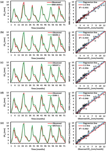
The temporal variation between simulated and observed monthly EP_m data, and their scatter plots (right side) for the MM-ANN-1, MARS-1, MGGP-1, SVM-1, and M5Tree-1 models was plotted in Figure 6 (a through e) for the testing period. In scatter plots, the regression line provided the coefficient of determination (R²) as 0.955 for the MM-ANN-1 model, 0.959 for the MARS-1 model, 0.956 for MGGP-1 model, 0.946 for SVM-1 model, and 0.962 for M5Tree-1 model during the testing stage, respectively. The fitted regression line (RL) and the perfect line of fit (1:1) were close to each other for all techniques. The RL was located above the best fit (1:1) for MARS-1, MGGP-1, SVM-1, and M5Tree-1 models. This means that at Pantnagar station, the five models over-predict the monthly pan evaporation values. Also, the regression line was located under the 1:1 line for MM-ANN-1 models, which means the model under-predict the pan evaporation values at Pantnagar station.

Figure 6. Line (left) and scatter (right) plots between observed and simulated monthly pan evaporation values by (a) MM-ANN-1, (b) MARS-1, (c) MGGP-1, (d) SVM-1, and (e) M5Tree-1 models during testing period at Pantnagar station.

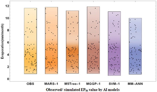
According to Figure 7, all model symbols were very close to each other. In detail, SVM-1 was located as the furthest from the observed point. This introduces SVM-1 as the worst model. MM-ANN-1 was the closest model to the observed point based on the standard deviation, correlation, and RMSE. The MM-ANN-1 model presented identical peaks and resembled the observed values (Figure 6(a)). This proves the superiority of the MM-ANN-1 model over the others. The density plots of the simulated EP_m by AI models against the observed (OBS) values are presented in Figure 8. However, the density plot suggested a slightly different distribution of the simulated values.

Figure 7. Taylor diagrams comparing the models’ fit statistics at Pantnagar station.

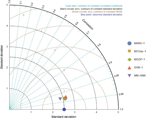
Figure 8. Density plots of MM-ANN, MARS-1, MGGP-1, SVM-1 and M5Tree-1 models at Pantnagar station.

3.3. Simulation of EP_m at Ranichauri station

The MM-ANN-1, MARS-1, MGGP-1, SVM-1 and M5Tree-1 models were trained using (January, 2000 to December, 2009) and tested using (2010 to December, 2012) datasets. The adequacy of these models was assessed using the NSE, WI, LM, RMSE and MAPE values in the both training and testing phases. Table 4 represents the NSE, WI, LM, RMSE and MAPE values for MM-ANN-1, MARS-1, MGGP-1, SVM-1 and M5Tree-1 models. As assessing Ranichauri station, NSE = 0.914, WI = 0.978, LM = 0.730, RMSE = 0.296 mm/ month and MAPE = 9.647% for MM-ANN-1 model; NSE = 0.927, WI = 0.981, LM = 0.766, RMSE = 0.272 mm/ month and MAPE = 8.028% for MARS-1 model; NSE = 0.887, WI = 0.969, LM = 0.677, RMSE = 0.339 mm/ month and MAPE = 12.631% for MGGP-1 model; NSE = 0.913, WI = 0.977, LM = 0.738, RMSE = 0.297 mm/ month and MAPE = 9.146% for SVM-1 model, and NSE = 0.905, WI = 0.974, LM = 0.724, RMSE = 0.310 mm/ month and MAPE = 9.595% for M5Tree-1 model were obtained during the training period. In addition, NSE = 0.909, WI = 0.975, LM = 0.736, RMSE = 0.368 mm/ month and MAPE = 10.633% for MM-ANN-1 model; NSE = 0.881, WI = 0.963, LM = 0.678, RMSE =0.421 mm/ month and MAPE=12.757% for MARS-1 model; NSE = 0.911, WI = 0.975, LM = 0.724, RMSE =0.364 mm/ month and MAPE=12.297% for MGGP-1 model; NSE = 0.811, WI = 0.955, LM = 0.598, RMSE =0.529 mm/ month and MAPE=18.096% for SVM-1 model, and NSE = 0.693, WI = 0.929, LM = 0.483, RMSE = 0.675 mm/ month and MAPE = 23.727% for M5Tree-1 model were obtained during the testing stage. Table 4 revealed that the MARS-1 model produced the best performances and results in the training stage while failed in the testing stage. The MGGP-1 model tracked the best statistical criteria (i.e. minimum RMSE and MAPE values, and maximum NSE, WI and LM values) over the testing stage and indicated the best performance compared to other models. MM-ANN-1 model follows the MGGP-1 as the second-best model.

The scatter plots and temporal variations graphs of the observed against the simulated EP_m of the MM-ANN-1, MARS-1, MGGP-1, SVM-1, and M5Tree-1 models over the testing phase were presented in Figure 9 (a through e). The RL in scatter plots marked R² as 0.910 for the MM-ANN-1, 0.910 for the MARS-1, 0.916 for the MGGP-1 model, 0.850 for SVM-1 model, and 0.852 for M5Tree-1 model over the testing period. The different conditions have been yielded between RL and 1:1 line for all the models. For the SVM-1 model (Figure 9(d)), the RL was exactly over the 1:1 line, it over-predicted the EP_m values. For the M5Tree-1 model (Figure 9(e)), the regression line was exactly below the best fit line (1:1), it under-predicted the EP_m values. In the case of MM-ANN-1, MARS-1 and MGGP-1 models (Figure 9(a–c)), the regression line divided the best fit line (1:1). It can be explained that the models over-predicted the smaller values (<2.5 mm/month for MM-ANN-1, <3.0 mm/month for MGGP-1, <2.5 mm/month for MARS-1) and under-predict the higher EP_m values at Ranichauri station.

Figure 9. Line (left) and scatter (right) plots between observed and simulated monthly pan evaporation values by (a) MM-ANN-1, (b) MARS-1, (c) MGGP-1, (d) SVM-1, and (e) M5Tree-1 models during testing period at Ranichauri station.

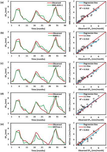
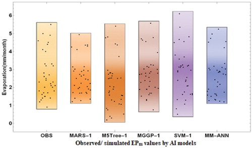
According to Figure 10, the highest correlation coefficient (CC) was observed in the MARS-1. But the standard deviation showed much less than the observed values. The SVM-1 and M5Tree-1 model is far from being competing on the best performance, MGGP-1 can be considered as a high performed model with lowest RMSE and high correlation although it has a standard deviation lower than the observed values. Finally, MGGP-1 was the closest model to the observed values based on the standard deviation, correlation, and RMSE. This was giving superiority to MGGP-1 over the others. Considering the density plot (Figure 11), the MGGP-1 model, which identified as the closest model in the Taylor diagram yielded a similar box from the observed values.

Figure 10. Taylor diagrams comparing the models’ fit statistics at Ranichauri station.

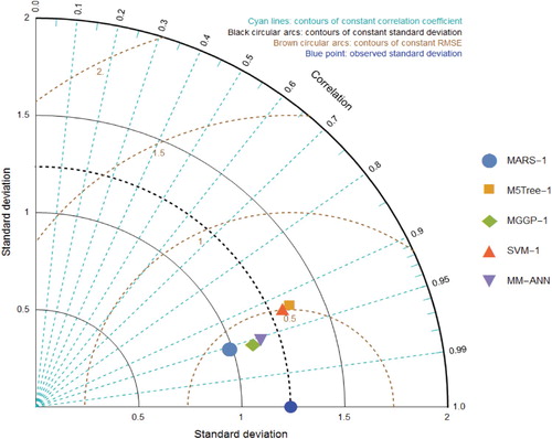
Figure 11. Density plots of MM-ANN, MARS-1, MGGP-1, SVM-1 and M5Tree-1 models at Ranichauri station.

The findings of the current research demonstrated that the MM-ANN at Pantnagar station and MGGP model at Ranichauri station achieved better performances in simulating EP_m values. The MM-ANN-1 and MGGP-1 models were selected as the best ones based on minimum RMSE and MAPE values, and maximum NSE, WI, and LM values at the testing period. Various researchers reported that the soft computing models provide better performances during the testing period, and the best performing procedure was selected (Abdullah, Malek, Abdullah, Kisi, & Yap, 2015; Guven & Kisi, 2013). Malik, Kumar, and Kisi (2017) estimated EP_m using SOMNN, CANFIS, MLPNN, RBNN, Griffith’s (G), and Stephens-Stewart (SS) models at Ranichauri and Pantnagar stations. They published that the specific heuristic approaches (i.e. MLPNN and CANFIS models) outperformed the other models. It can be clear that the previous investigations confirmed the multiple model strategies for modeling nonlinear time series phenomena. The findings of this research were also in close agreement with the study done by (Malik, Kumar, & Kisi, 2017). Future research can be devoted to the incorporation of other casual related climate variables such as vapor pressure deficit, atmospheric pressure or others.

4. Conclusion

The evaporation process of the hydrological cycle is characterized by highly complex and stochastic phenomena in nature. In the current research, the ability of multiple model strategies (MM-ANN, MARS, MGGP, SVM, and M5Tree) was evaluated in simulating monthly pan evaporation at two meteorological stations, Ranichauri and Pantnagar in India. The best input variables combination was selected using GT. The results of applied models were examined using some performance criteria and visual presentations. In general, we derived five conclusions from the current research as follows:

• Six appropriate variables (RH₁, RH₂, S_w, H_ss, and T_min, T_max,) were selected by GT as the optimistic input combination for simulating the pan evaporation in monthly scale at both studied stations. The nature of the EP_m process in this region is highly stochastic and more climatic information is needed for building the prediction matrix of the proposed AI models.

• At the Pantnagar station, the MM-ANN-1 model indicated the better performance compared to the MARS-1, MGGP-1, SVM-1 and M5Tree-1 models. However, the feasibility of the MGGP-1 model demonstrated batter results at Ranichauri station. This is normal for the case where AI models behave differently in different cases based on the actual internal mechanism between the predictand and predictors.

• MARS model performed as the second accurate model following the MM-ANN at Pantnagar station, while the MM-ANN was following the MGGP model capacity in mimicking the EP_m trend at Ranichauri station.

• Overall, the attained results of the proposed MM-ANN and MGGP models demonstrated an optimistic intelligence approaches for this particular region where they would contribute to the water resources engineering practice, and management.

Disclosure statement

No potential conflict of interest was reported by the authors.

References

- Abdullah, S. S., Malek, M. a., Abdullah, N. S., Kisi, O., & Yap, K. S. (2015). Extreme learning machines: A new approach for prediction of reference evapotranspiration. Journal of Hydrology, 527, 184–195. doi: 10.1016/j.jhydrol.2015.04.073
- Adamowski, J., Chan, H. F., Prasher, S. O., & Sharda, V. N. (2012). Comparison of multivariate adaptive regression splines with coupled wavelet transform artificial neural networks for runoff forecasting in Himalayan micro-watersheds with limited data. Journal of Hydroinformatics, 14(3), 731–744. doi: 10.2166/hydro.2011.044
- Adnan, R. M., Malik, A., Kumar, A., Parmar, K. S., & Kisi, O. (2019). Pan evaporation modeling by three different neuro-fuzzy intelligent systems using climatic inputs. Arabian Journal of Geosciences, 12(20), 606. doi: 10.1007/s12517-019-4781-6
- Burt, C. M., Mutziger, A. J., Allen, R. G., & Howell, T. A. (2005). Evaporation research: Review and interpretation. Journal of Irrigation and Drainage Engineering, 131(1), 37–58. doi: 10.1061/(ASCE)0733-9437(2005)131:1(37)
- Danandeh Mehr, A., & Kahya, E. (2017). A Pareto-optimal moving average multigene genetic programming model for daily streamflow prediction. Journal of Hydrology, 549, 603–615. doi: 10.1016/j.jhydrol.2017.04.045
- Danandeh Mehr, A., Kahya, E., & Olyaie, E. (2013). Streamflow prediction using linear genetic programming in comparison with a neuro-wavelet technique. Journal of Hydrology, 505, 240–249. doi: 10.1016/j.jhydrol.2013.10.003
- Danandeh Mehr, A., Kahya, E., & Yerdelen, C. (2014). Linear genetic programming application for successive-station monthly streamflow prediction. Computers and Geosciences, 70, 63–72. doi: 10.1016/j.cageo.2014.04.015
- Danandeh Mehr, A., & Nourani, V. (2017). A Pareto-optimal moving average-multigene genetic programming model for rainfall-runoff modelling. Environmental Modelling and Software, 92, 239–251. doi: 10.1016/j.envsoft.2017.03.004
- De Andrés, J., Lorca, P., de Cos Juez, F. J., & Sánchez-Lasheras, F. (2011). Bankruptcy forecasting: A hybrid approach using Fuzzy c-means clustering and multivariate adaptive regression Splines (MARS). Expert Systems with Applications, 38(3), 1866–1875. doi: 10.1016/j.eswa.2010.07.117
- Deo, R. C., Kisi, O., & Singh, V. P. (2017). Drought forecasting in eastern Australia using multivariate adaptive regression spline, least square support vector machine and M5Tree model. Atmospheric Research, 184, 149–175. doi: 10.1016/j.atmosres.2016.10.004
- Deo, R. C., Samui, P., & Kim, D. (2016). Estimation of monthly evaporative loss using relevance vector machine, extreme learning machine and multivariate adaptive regression spline models. Stochastic Environmental Research and Risk Assessment, 30(6), 1769–1784. doi: 10.1007/s00477-015-1153-y
- Doorenbos, J., & Pruitt, W. O. (1977). Guidelines for predicting crop water requirements (Irrigation and Drainage Paper No. 24, FAO). doi: 10.2514/6.2014-2117
- Friedman, J. H. (1991). Multivariate adaptive regression Splines. The Annals of Statistics, 19, 1–67. doi: 10.1214/aos/1176347963
- Ghorbani, M. A., Deo, R. C., Yaseen, Z. M., Kashani, M. H., & Mohammadi, B. (2017). Pan evaporation prediction using a hybrid multilayer perceptron-firefly algorithm (MLP-FFA) model: Case study in North Iran. Theoretical and Applied Climatology, 133, 1119–1131. doi: 10.1007/s00704-017-2244-0
- Ghorbani, M. A., Khatibi, R., Karimi, V., Yaseen, Z. M., & Zounemat-Kermani, M. (2018). Learning from multiple models using artificial intelligence to Improve model prediction accuracies: Application to river flows. Water Resources Management, 32, 4201–4215. doi: 10.1007/s11269-018-2038-x
- Goyal, M. K. (2014). Modeling of sediment yield prediction using M5 model tree algorithm and wavelet regression. Water Resources Management 28, 1991–2003. doi: 10.1007/s11269-014-0590-6
- Goyal, M. K., Bharti, B., Quilty, J., Adamowski, J., & Pandey, A. (2014). Modeling of daily pan evaporation in sub tropical climates using ANN, LS-SVR, Fuzzy Logic, and ANFIS. Expert Systems with Applications, 41(11), 5267–5276. doi: 10.1016/j.eswa.2014.02.047
- Griffiths, J. F. (1966). Another evaporation formula. Agricultural Meteorology, 3(3–4), 257–261. doi: 10.1016/0002-1571(66)90033-1
- Guven, A. (2009). Linear genetic programming for time-series modelling of daily flow rate. Journal of Earth System Science, 118(2), 137–146. doi: 10.1007/s12040-009-0022-9
- Guven, A., & Kisi, O. (2013). Monthly pan evaporation modeling using linear genetic programming. Journal of Hydrology, 503, 178–185. doi: 10.1016/j.jhydrol.2013.08.043
- Kashani, M. H., Ghorbani, M. A., Shahabi, M., Naganna, S. R., & Diop, L. (2020). Multiple AI model integration strategy—application to saturated hydraulic conductivity prediction from easily available soil properties. Soil and Tillage Research, 196, 104449. doi: 10.1016/j.still.2019.104449
- Keshtegar, B., Piri, J., & Kisi, O. (2016). A nonlinear mathematical modeling of daily pan evaporation based on conjugate gradient method. Computers and Electronics in Agriculture, 127, 120–130. doi: 10.1016/j.compag.2016.05.018
- Khatibi, R., Ghorbani, M. A., Jani, R., & Servati, M. (2018). Soil cation exchange capacity predicted by learning from multiple modelling: Forming multiple models run by SVM to Learn from ANN and its hybrid with firefly algorithm. In D. Kim, R. Deo, & P. Samui (Eds.), Handbook of research on predictive modeling and optimization methods in science and engineering (pp. 465–480). Hershey, PA: IGI Global.
- Khatibi, R., Ghorbani, M. A., & Pourhosseini, F. A. (2017). Stream flow predictions using nature-inspired firefly algorithms and a multiple model strategy–directions of innovation towards next generation practices. Advanced Engineering Informatics, 34, 80–89. doi: 10.1016/j.aei.2017.10.002
- Kisi, O. (2015). Pan evaporation modeling using least square support vector machine, multivariate adaptive regression splines and M5 model tree. Journal of Hydrology, 528, 312–320. doi: 10.1016/j.jhydrol.2015.06.052
- Kişi, O., & Cimen, M. (2009). Evapotranspiration modelling using support vector machines/Modélisation de l’évapotranspiration à l’aide de ‘support vector machines’. Hydrological Sciences Journal, 54(5), 918–928. doi: 10.1623/hysj.54.5.918
- Kisi, O., Genc, O., Dinc, S., & Zounemat-Kermani, M. (2016). Daily pan evaporation modeling using chi-squared automatic interaction detector, neural networks, classification and regression tree. Computers and Electronics in Agriculture, 122, 112–117. doi: 10.1016/j.compag.2016.01.026
- Kisi, O., & Heddam, S. (2019). Evaporation modelling by heuristic regression approaches using only temperature data. Hydrological Sciences Journal, 64(6), 653–672. doi: 10.1080/02626667.2019.1599487
- Malik, A., & Kumar, A. (2015). Pan evaporation simulation based on daily meteorological data using soft computing techniques and multiple linear regression. Water Resources Management, 29(6), 1859–1872. doi: 10.1007/s11269-015-0915-0
- Malik, A., & Kumar, A. (2018). Comparison of soft-computing and statistical techniques in simulating daily river flow: A case study in India. Journal of Soil and Water Conservation, 17(2), 192. doi: 10.5958/2455-7145.2018.00029.2
- Malik, A., Kumar, A., Ghorbani, M. A., Kashani, M. H., Kisi, O., & Kim, S. (2019). The viability of co-active fuzzy inference system model for monthly reference evapotranspiration estimation: Case study of Uttarakhand State. Hydrology Research, 50, 1623–1644. doi: 10.2166/nh.2019.059
- Malik, A., Kumar, A., & Kisi, O. (2017). Monthly pan-evaporation estimation in Indian central Himalayas using different heuristic approaches and climate based models. Computers and Electronics in Agriculture, 143, 302–313. doi: 10.1016/j.compag.2017.11.008
- Malik, A., Kumar, A., & Kisi, O. (2018). Daily Pan evaporation estimation using heuristic methods with gamma test. Journal of Irrigation and Drainage Engineering, 144(9), 04018023. doi: 10.1061/(asce)ir.1943-4774.0001336
- Malik, A., Kumar, A., & Singh, R. P. (2019). Application of heuristic approaches for prediction of hydrological drought using multi-scalar streamflow drought index. Water Resources Management, 33, 3985–4006. doi: 10.1007/s11269-019-02350-4
- Moghaddamnia, a., Ghafari Gousheh, M., Piri, J., Amin, S., & Han, D. (2009). Evaporation estimation using artificial neural networks and adaptive neuro-fuzzy inference system techniques. Advances in Water Resources, 32(1), 88–97. doi: 10.1016/j.advwatres.2008.10.005
- Penman, H. L. (1948). Natural evaporation from open water, bare soil and grass. Proceedings of the Royal Society of London. Series A. Mathematical and Physical Sciences, 193(1032), 120–145. doi: 10.1098/rspa.1948.0037
- Piri, J., Amin, S., Moghaddamnia, A., Keshavarz, A., Han, D., & Remesan, R. (2009). Daily pan evaporation modeling in a hot and dry climate. Journal of Hydrologic Engineering, 14(8), 803–811. doi: 10.1061/(ASCE)HE.1943-5584.0000056
- Priestley, C. H. B., & Taylor, R. J. (1972). On the assessment of the surface heat flux and evaporation using large-scale parameters. Monthly Weather Review, 100, 81–92. doi: 10.1175/1520-0493(1972)100<0081:OTAOSH>2.3.CO;2
- Qasem, S. N., Samadianfard, S., Kheshtgar, S., Jarhan, S., Kisi, O., Shamshirband, S., & Chau, K.-W. (2019). Modeling monthly pan evaporation using wavelet support vector regression and wavelet artificial neural networks in arid and humid climates. Engineering Applications of Computational Fluid Mechanics, 13(1), 177–187. doi: 10.1080/19942060.2018.1564702
- Qutbudin, I., Shiru, M. S., Sharafati, A., Ahmed, K., Al-Ansari, N., Yaseen, Z. M., … Wang, X. (2019). Seasonal drought pattern changes Due to climate variability: Case study in Afghanistan. Water, 11(5), 1096. doi: 10.3390/w11051096
- Rahimikhoob, A. (2014). Comparison between M5 model tree and neural networks for estimating reference evapotranspiration in an arid environment. Water Resources Management, 28(3), 657–669. doi: 10.1007/s11269-013-0506-x
- Remesan, R., Shamim, M. A., & Han, D. (2008). Model data selection using gamma test for daily solar radiation estimation. Hydrological Processes, 22(21), 4301–4309. doi: 10.1002/hyp.7044
- Remesan, R., Shamim, M. A., Han, D., & Mathew, J. (2009). Runoff prediction using an integrated hybrid modelling scheme. Journal of Hydrology, 372(1–4), 48–60. doi: 10.1016/j.jhydrol.2009.03.034
- Rezaie-Balf, M., Kisi, O., & Chua, L. H. C. (2019). Application of ensemble empirical mode decomposition based on machine learning methodologies in forecasting monthly pan evaporation. Hydrology Research, 50(2), 498–516. doi: 10.2166/nh.2018.050
- Salih, S. Q., sharafati, A., Khosravi, K., Faris, H., Kisi, O., Tao, H., … Yaseen, Z. M. (2020). River suspended sediment load prediction based on river discharge information: Application of newly developed data mining models. Hydrological Sciences Journal. doi: 10.1080/02626667.2019.1703186
- Searson, D. P. (2015). GPTIPS 2: An open-source software platform for symbolic data mining. In Handbook of genetic programming applications (pp. 551–573). doi: 10.1007/978-3-319-20883-1_22
- Sebbar, A., Heddam, S., & Djemili, L. (2019). Predicting daily Pan evaporation (Epan) from Dam reservoirs in the mediterranean regions of Algeria: OPELM vs OSELM. Environmental Processes, 6, 309–319. doi: 10.1007/s40710-019-00353-2
- Sharafati, A., Khosravi, K., Khosravinia, P., Ahmed, K., Salman, S. A., Mundher, Z., & Shamsuddin, Y. (2019). The potential of novel data mining models for global solar radiation prediction. International Journal of Environmental Science and Technology, 0123456789. doi: 10.1007/s13762-019-02344-0
- Sharafati, A., Tafarojnoruz, A., Shourian, M., & Yaseen, Z. M. (2019). Simulation of the depth scouring downstream sluice gate: The validation of newly developed data-intelligent models. Journal of Hydro-Environment Research. doi: 10.1016/j.jher.2019.11.002
- Sharafati, A., Yasa, R., & Azamathulla, H. M. (2018). Assessment of stochastic approaches in prediction of wave-induced pipeline scour depth. Journal of Pipeline Systems Engineering and Practice, 9(4), 04018024. doi: 10.1061/(ASCE)PS.1949-1204.0000347
- Shoaib, M., Shamseldin, A. Y., Melville, B. W., & Khan, M. M. (2015). Runoff forecasting using hybrid wavelet gene expression programming (WGEP) approach. Journal of Hydrology, 527, 326–344. doi: 10.1016/j.jhydrol.2015.04.072
- Singh, A., Malik, A., Kumar, A., & Kisi, O. (2018). Rainfall-runoff modeling in hilly watershed using heuristic approaches with gamma test. Arabian Journal of Geosciences, 11(11). doi: 10.1007/s12517-018-3614-3
- Singh, K. K., Pal, M., & Singh, V. P. (2010). Estimation of mean annual flood in Indian catchments using backpropagation neural network and M5 model tree. Water Resources Management, 24(10), 2007–2019. doi: 10.1007/s11269-009-9535-x
- Tabari, H., Talaee, P. H., & Abghari, H. (2012). Utility of coactive neuro-fuzzy inference system for pan evaporation modeling in comparison with multilayer perceptron. Meteorology and Atmospheric Physics, 116(3–4), 147–154. doi: 10.1007/s00703-012-0184-x
- Tao, H., Diop, L., Bodian, A., Djaman, K., Ndiaye, P. M., & Yaseen, Z. M. (2018). Reference evapotranspiration prediction using hybridized fuzzy model with firefly algorithm: Regional case study in Burkina Faso. Agricultural Water Management, 208, 140–151. doi: 10.1016/j.agwat.2018.06.018
- Tikhamarine, Y., Malik, A., Kumar, A., Souag-Gamane, D., & Kisi, O. (2019). Estimation of monthly reference evapotranspiration using novel hybrid machine learning approaches. Hydrological Sciences Journal, 64(15), 1824–1842. doi: 10.1080/02626667.2019.1678750
- Tsui, A. P. M., Jones, A. J., & De Oliveira, A. G. (2002). The construction of smooth models using irregular embeddings determined by a gamma test analysis. Neural Computing & Applications, 10(4), 318–329. doi: 10.1007/s005210200004
- Wang, L., Kisi, O., Hu, B., Bilal, M., Zounemat-Kermani, M., & Li, H. (2017). Evaporation modelling using different machine learning techniques. International Journal of Climatology, 37(S1), 1076–1092. doi: 10.1002/joc.5064
- Wang, L., Kisi, O., Zounemat-Kermani, M., & Li, H. (2017). Pan evaporation modeling using six different heuristic computing methods in different climates of China. Journal of Hydrology, 544, 407–427. doi: 10.1016/j.jhydrol.2016.11.059
- Wang, L., Niu, Z., Kisi, O., Li, C., & Yu, D. (2017). Pan evaporation modeling using four different heuristic approaches. Computers and Electronics in Agriculture, 140, 203–213. doi: 10.1016/j.compag.2017.05.036
- Yaseen, Z. M., Al-Juboori, A. M., Beyaztas, U., Al-Ansari, N., Chau, K.-W., Qi, C., … Shahid, S. (2019). Prediction of evaporation in arid and semi-arid regions: A comparative study using different machine learning models. Engineering Applications of Computational Fluid Mechanics, 14(1), 70–89. doi: 10.1080/19942060.2019.1680576
- Yaseen, Z. M., El-shafie, A., Jaafar, O., Afan, H. A., & Sayl, K. N. (2015). Artificial intelligence based models for stream-flow forecasting: 2000–2015. Journal of Hydrology, 530, 829–844. doi: 10.1016/j.jhydrol.2015.10.038
- Zorn, C. R., & Shamseldin, A. Y. (2015). Peak flood estimation using gene expression programming. Journal of Hydrology, 531, 1122–1128. doi: 10.1016/j.jhydrol.2015.11.018