One-dimensional and three-dimensional computational thermal fluid hybrid analysis-aided air distribution pipeline system design

Abstract

The air distribution system is an essential aircraft system, helping to create a safe, healthy and thermally comfortable cabin environment for large-scale aircraft. This complex pipe network system contains a large number of pipes, valves, elbows, joints and flow devices. The enormous number of components poses a severe challenge to the efficiency, accuracy and convergence of system thermal fluid analysis. Traditional three-dimensional (3D) computational fluid dynamics (CFD) methods can describe the system internal flow and heat transfer performance in detail with complex mesh models and extremely low calculation efficiency, while one-dimensional (1D) fluid system simulation methods have better computational efficiency but insufficient calculation accuracy. This study proposes a method to implement efficient and accurate simulation to solve this problem. 1D fluid system analysis models are established to obtain the P-Q characteristic curve of each pipeline subsystem. These 1D models are also used to evaluate the uniformity of air flow into each compartment of the aircraft cabin and the thermal insulation performance of system pipelines. The 3D CFD model is built to evaluate the air distribution performance of the mix manifold using the subsystem P-Q characteristics as the boundary conditions. The air distribution analysis based on the CFD model is compared with that using the 1D fluid system model in the same boundary conditions. The results show that more than 7% deviation occurs if the influence of the mix manifold structure on its internal flow is ignored.

KEYWORDS:

• Large-scale aircraft
• air distribution
• pipeline system
• 1D thermal fluid system analysis
• CFD

1. Introduction

The air distribution system is a pipe network system that supplies conditioned air from the mix manifold to the aircraft cabin. It is an essential aircraft system needed to create a safe, healthy and thermally comfortable cabin environment. A large number of research works, including experiments and numerical simulations, have been conducted to find an optimal ventilation mode to save energy and improve the air quality and thermal comfort of the aircraft cabin. Zhang and Chen (2007) proposed an underfloor displacement air distribution system and a personalized air distribution system, comparing the air and contaminant distributions in a Boeing 767 aircraft cabin using a computational fluid dynamics (CFD) program, and concluded that the personalized air distribution system provided the best air quality with no draft risk. Zítek, Vyhlídal, Simeunović, Nováková, and Čížek (2010) proposed a micro-environment control system consisting of supplying each of the passengers with her or his own supply of fresh, humidified air. This system was designed based on CFD models and verified by means of laboratory experiments. Pang et al. (2013) proposed an improved air distribution system with personalized outlets placed at the bottom of the baggage hold. Simulations revealed that this improved pattern had the potential to save energy by decreasing the amount of fresh air without significantly affecting air quality and thermal comfort. Cao et al. (2014) performed a large-scale particle image velocimetry (PIV) measurement to characterize the mixing air distributions inside a partly transparent aircraft cabin mock-up. You et al. (2016) conducted experimental measurements of airflow distribution in a mock-up of half of a full-scale, one-row, single-aisle aircraft cabin with a gasper on. However, very few studies on air ventilation pipelines, which also play an important part in thermal comfort and energy economy in the aircraft cabin, have been carried out. The air distribution system should first be designed to meet the fresh air demands of cabin passengers by controlling the air distribution proportion for each cabin compartment. It is also necessary to control the uniformity of the air flow rate of each air outlet into the cabin to ensure the thermal comfort of different cabin regions. To guarantee that the conditioned air still has sufficient heating or cooling capacity when it reaches the branch outlets, insulation of the pipeline needs to be considered and designed.

The air distribution system of commercial aircraft is a complex pipe network system, including hundreds of components such as pipes, joints, bends and orifices. It is difficult to reach convergence in this system analysis owing to the huge number of components of the simulation model. CFD software (Park, Park, & Lee, 2016; Poussou, Mazumdar, Plesniak, Sojka, & Chen, 2010) and MATLAB® program (Eero-Matti & Holopainen, 2008; Tibor, Lawrence, & John, 2013) are traditionally used to analyze the system flow and thermal performance. However, neither of these methods has satisfactory computational efficiency for the performance analysis of complex multi-element fluid systems. The one-dimensional (1D) thermal fluid analysis software Flowmaster is widely used in complex fluid systems analysis, such as fuel, hydraulic and air conditioning systems in the aviation field (Ng & Tan, 2009; Shi et al., 2013; Tu & Lin, 2011); this is based on the linearization coefficients method of the models, and possesses superior convergence properties compared with the MATLAB program. However, the Flowmaster software cannot describe the internal flow details of each component, and when facing hundreds of component-level system analyses, engineers using this software tend to ignore the effects of the internal structure of some components on the flow characteristics, to improve computational efficiency and convergence (Shayne & Mentor Graphics, 2009; Tu & Lin, 2011). For example, when simulating the air distribution system, the mix manifold is normally treated as a calculation node with conservation of mass and energy. This simplified method usually causes a reduction in the calculation accuracy.

Three-dimensional (3D) CFD is a powerful method in modeling various components to obtain the internal or external flow and thermal behavior for solving engineering problems. Mou, He, Zhao, and Chau (2017) used CFD to ascertain wind pressure distributions on and around squared-shaped tall buildings. Ramezanizadeh, Mohammad, Mohammad, and Chau (2019) compared the performance of a thermosyphon heat exchanger with a copper material type, based on experimental and CFD analysis. Akbarian et al. (2018) used a CFD method to simulate the use of natural gas in a dual-fueled diesel engine. Li, Ji, Shi, and Sun (2019) used CFD to numerically evaluate the influence of the rotor–stator partition structure on the aerodynamic performance of the centrifugal compressor and its loss mechanism. It can be seen from the above research and applications that CFD is an important engineering method for describing the flow and heat transfer inside or outside the equipment, especially for complicated structural components.

This paper studies a hybrid design method for large-scale aircraft air distribution systems by jointly using 1D and 3D fluid analysis. The 1D thermal and fluid analysis models of the subsystems are established first. Then, the flow distribution and pressure drop characteristics of each subsystem are calculated and the thermal insulation performance of the pipelines is evaluated. Based on these investigations, the pressure drop–flow characteristics of all subsystems are obtained and used to set the boundary conditions for the mix manifold CFD model to analyze the air distribution performance among the subsystems. A comparative analysis is carried out for the mix manifold system using a 1D method and a 3D CFD model to determine the influence of internal structure on the flow distribution of the mix manifold.

2. System introduction

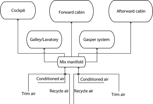
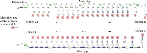
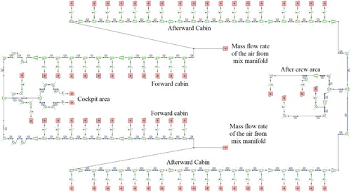
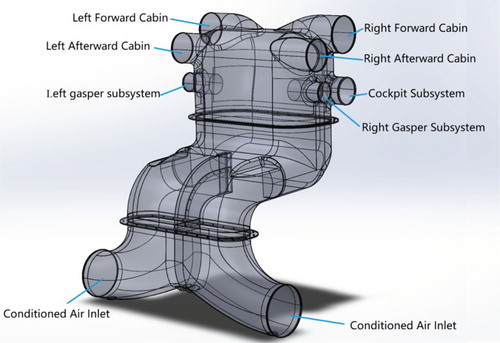
Most commercial aircraft use an air-cycle machine (ACM) as a source of cool air. The cooled air from the ACM is mixed with the high-temperature bleed air from the engine to adjust its temperature. Considering the fuel efficiency, a certain percentage of cabin air will be recycled to maintain enough fresh air for the cabin passengers. These three sources of air are conveyed into the mix manifold and mixed thoroughly, then supplied to the different compartments of the aircraft, including the cockpit, forward cabin, afterward cabin, galley, lavatory and individual gaspers, as shown in Figure 1. Separate main pipes are used to extract air from the mix manifold for each compartment, and the conditioned air drawn from the mixer is distributed to various locations in the aircraft compartments through branch pipes. Each independent pipeline from the mix manifold can be considered as a subsystem.

Figure 1. Schematic diagram of the air distribution system for a large aircraft.

To ensure that all compartments of the aircraft have enough fresh air for passengers to breathe, as required by section 25.831 of China Civil Aviation Regulations (CAAC, 2011), and cabin temperature control, each distribution subsystem has a total mass flow demand. The flow resistance of subsystems will affect their respective flow distribution proportions. Therefore, the relative flow resistance of each subsystem needs to be designed and matched to ensure enough mass flow for each subsystem in the case of a constant total air flow rate for the whole air distribution system.

For the thermal comfort of passengers, the air distribution system needs to be designed to ensure the uniformity of branch air flow. The flow deviation among branch outlets of the subsystem is generally specified within ±5%. To improve the comfort of the aircraft and meet the airline’s operational requirements, the aerospace recommended practice of the Society of Automotive Engineers (SAE, 2012) suggests that during ground operations, the system should be capable of heating the cabin on the ground to an average temperature of 21°C within 30 min, starting with a cold soaked airplane at a temperature of −32°C, and the system should be capable of cooling the cabin on the ground to an average temperature of 27°C within 30 min, starting with a cabin temperature of 46°C. This not only requires that the air conditioning system of an aircraft has sufficient heating or cooling capacity, but also requires the air distribution pipelines to have enough thermal insulation for energy economy considerations. This makes severe demands on the insulation performance of the mix manifold and the air distribution pipeline to ensure that the heat (or coldness) of the conditioned air is not lost during transmission and that it maintains its maximum temperature regulating ability.

3. Subsystem modeling and analysis

3.1. Main component model

Flowmaster contains a large number of standard components that can be directly used by consumers. The flow characteristics of most of these components are based on the experimental data of the British Association for Fluid Dynamics Research, which are summarized in Miller (1984).

3.1.1. Pipe model

The pressure loss along a pipe of a given length with average velocity can be calculated using the Darcy–Weisbach equation: (1) $\mathrm{\Delta }p=\frac{fL}{d}\cdot \frac{{\text{m}}^2}{2\rho A^2}$(1) where L = pipe length; A = pipe cross-sectional area; ρ = fluid density; d = pipe diameter; m = mass flow rate through the pipe; and f = Darcy friction factor.

The friction factor is calculated using Equation (2(2) $\mathrm{Re}\le 2000,f=f_{\text{l}}=\frac{64}{\mathrm{Re}}$(2) ) for laminar flow conditions (Re ≤ 2000): (2) $\mathrm{Re}\le 2000,f=f_{\text{l}}=\frac{64}{\mathrm{Re}}$(2)

The approximation Colebrook–White equation is used to estimate the Darcy friction factor for turbulent flow (Re > 4000) in pipes, as in Equation (3(3) $\mathrm{Re}\ge 4000,f=f_t=\frac{0.25}{{\left[\log \left(\frac{k}{3.7D}+\frac{\text{5}\text{.74}}{\text{R}{\text{e}}^{\text{0}\text{.9}}}\right)\right]}^2}$(3) ): (3) $\mathrm{Re}\ge 4000,f=f_t=\frac{0.25}{{\left[\log \left(\frac{k}{3.7D}+\frac{\text{5}\text{.74}}{\text{R}{\text{e}}^{\text{0}\text{.9}}}\right)\right]}^2}$(3) where f_t = friction factor of turbulent conditions; and k/D = relative roughness. This equation was checked for accuracy with the Colebrook–White equation, and it was found that for 10⁻⁶≤ k/D ≤ 10⁻² and 5 × 10³≤ Re ≤ 10⁸, the errors involved in the friction factor are well within ±1.0%, with reference to Swamee and Jain (1976).

For transitional flow conditions (2000 < Re ≤ 4000), linear interpolation is applied from f_l to f_t, as in Equation (4(4) $2000<\mathrm{Re}\le 4000,f=\frac{\mathrm{Re}-2000}{2000}{f}_t+\frac{\text{4}000-\mathrm{Re}}{2000}{f}_l$(4) ): (4) $2000<\mathrm{Re}\le 4000,f=\frac{\mathrm{Re}-2000}{2000}{f}_t+\frac{\text{4}000-\mathrm{Re}}{2000}{f}_l$(4)

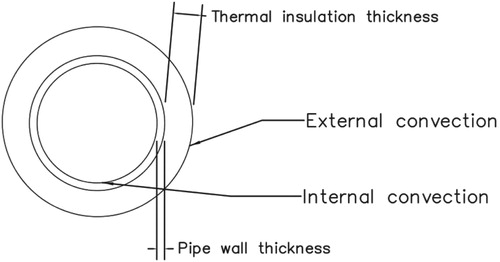
As shown in Figure 2, four parts of thermal resistance should be considered when calculating the heat insulation performance of a pipe. The total thermal resistance can be calculated by Equation (5(5) $R=\frac{1}{{\lambda }_w{\delta }_w}+\frac{1}{{\lambda }_e{\delta }_e}+\frac{1}{h_e}+\frac{1}{h_{\text{i}}}$(5) ): (5) $R=\frac{1}{{\lambda }_w{\delta }_w}+\frac{1}{{\lambda }_e{\delta }_e}+\frac{1}{h_e}+\frac{1}{h_{\text{i}}}$(5) where ${\lambda }_w$ = thermal conductivity of pipe wall material; ${\lambda }_e$ = thermal conductivity of insulation material; ${\delta }_w$ = pipe wall thickness; ${\delta }_e$ = thermal insulation thickness; h_e = pipe external convective heat transfer coefficient; and h_i = pipe internal convective heat transfer coefficient. The thermal resistance of the insulation layer is the largest of the four parts, while the thermal resistance of internal convection is relatively small and can normally be neglected.

Figure 2. Pipe thermal insulation layers.

3.1.2. Discrete loss model

A discrete loss model is used to simulate the irregular pipe resistance using Equation (6(6) $\mathrm{\Delta }p=K\cdot \frac{{\text{m}}^2}{2\rho A^2}$(6) ): (6) $\mathrm{\Delta }p=K\cdot \frac{{\text{m}}^2}{2\rho A^2}$(6) where K = loss coefficient, which can be obtained by experimentation or CFD analysis.

3.2. Subsystem modeling

The present system-level numerical analyses were performed using the 1D CFD software Flowmaster version 7.9.5. The compressible steady state is chosen as the simulation type for the system analysis. The working fluid used in this calculation is air.

As there is no crossing flow between the subsystems, the flow distribution and thermal insulation performance can be designed independently for each subsystem. The simulation model of the subsystem needs to be established according to the actual pipeline structure design. Owing to the influence of aircraft structure design, there are multiple abnormally shaped pipes in the air distribution pipeline. These components should first be analyzed by the CFD method to obtain their pressure drop and flow characteristics, and then modeled in the system using the discrete loss component model.

3.2.1. Cockpit distribution subsystem model

A 1D fluid subsystem analysis model of cockpit distribution is established, as shown in Figure 3. A flow source component model is used to set the total air mass flow rate of the cockpit subsystem, with an analysis range of 0–0.3 kg/s. Pressure source components are used as the outlet boundary of this case, which are set to sea-level pressure, i.e. 101,325 Pa. The diameter of the main pipe decreases from 0.102 to 0.0576 m along the flow direction. The pipeline branches are equipped with orifices with diameter between 0.028 and 0.04 m to balance the flow rate among all air outlets. The discrete loss components are used to model the irregular pipes in this pipeline system and their hydraulic characteristics can be obtained through local CFD simulations. In this analysis, the loss coefficient of the discrete loss component was set to 0.6 and the hydraulic diameter is consistent with their upstream pipes.

Figure 3. One-dimensional analysis model of the cockpit air distribution system.

3.2.2. Forward cabin distribution subsystem model

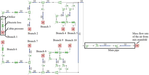
As shown in Figure 4, the main pipe is arranged along the fuselage axial direction to convey the air from the mix manifold to various positions in the forward cabin using branches along the main pipes. A flow source component model is used to set the total air mass flow rate of the forward cabin subsystem, with an analysis range of 0–1 kg/s. Pressure source components are used to set the outlet boundary with the sea-level pressure of 101,325 Pa. The diameter of the main pipe decreases along the flow direction from 0.127 to 0.0508 m, with six gradual pipes used for the transition. The diameter of the branch pipes is 0.038 m and the branch pipes are also equipped with orifices with diameter between 0.0248 and 0.0295 m to balance the flow rate among all air outlets.

Figure 4. One-dimensional analysis model of the forward cabin air distribution subsystem.

3.2.3. Afterward cabin distribution subsystem model

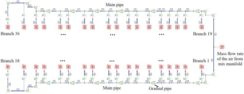
The afterward cabin air distribution pipeline is independent of the forward cabin subsystem. It has separate main pipes to transmit air from the mix manifold to the afterward cabin. As shown in Figure 5, a flow source component model is used to set the total air mass flow rate of the forward cabin subsystem, with an analysis range of 0–1 kg/s. Pressure source components are used to set the outlet boundary with the sea-level pressure of 101,325 Pa. The diameter of the main pipe decreases along the flow direction from 0.158 to 0.0762 m, with gradual pipes used for the transition. The diameter of the branch pipes is 0.038 m and the branches are equipped with orifices with diameter between 0.0252 and 0.0265 m to balance the flow rate among all air outlets. The irregular pipes are modeled by discrete loss components. The loss coefficient of these components was set to 0.4 and the hydraulic diameter is consistent with their upstream pipes in this analysis.

Figure 5. One-dimensional analysis model of the afterward cabin air distribution subsystem.

3.2.4. Gasper distribution subsystem model

The gasper distribution system conveys air from the mix manifold to the forward cabin, afterward cabin, galley, lavatory and cockpit for individual ventilation. The gasper system extracts air from the mix manifold directly, as in the other subsystems. As shown in Figure 6, flow source components are used to set the total air mass flow rate of the gasper distribution subsystem, with an analysis range of 0–0.5 kg/s. Pressure source components are used to set the outlet boundary with the sea-level pressure of 101,325 Pa. Junction components are used to model the air bleed opening on the main pipe, with arm diameter 0.024 m and angle 45°. The pipeline branches are equipped with orifices with diameter between 0.0137 and 0.0176 m to balance the flow rate among all air outlets.

Figure 6. One-dimensional analysis model of the individual cabin air distribution subsystem.

3.3. Pressure drop and flow characteristics analysis of each subsystem

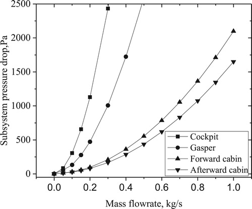
The results of the pipeline system pressure drops versus flow characteristics are shown in Figure 7. These characteristic curves are obtained by calculating the total pressure drops of each subsystem under different mass flow rates using the 1D models established in Section 3.2. As can be seen from Figure 7, the cockpit subsystem has the largest flow resistance, while the afterward cabin subsystem has the lowest flow resistance. This also means that the air distribution proportion of the afterward cabin subsystem will be the largest and the cockpit will be the smallest under the same pressure boundary of the system inlet and outlet.

Figure 7. Pressure drop–flow characteristics curve of the air distribution subsystem.

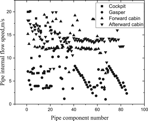
To control the noise in the cabin, it is necessary to limit the velocity of air in the pipeline, normally to less than 20 m/s. The internal air flow velocity of the system pipes can also be calculated using these 1D models. Figure 8 shows the air flow velocity inside all supply pipes under the design conditions. This parameter should be checked and evaluated during the system design, which can also be done by the subsystem 1D model.

Figure 8. Internal flow-velocity distribution of the air distribution subsystem pipe.

3.4. Flow deviation and thermal insulation performance of each subsystem

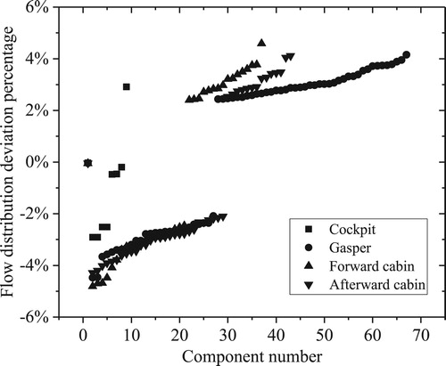
For consideration of passenger comfort, air distribution subsystems should be designed to ensure the uniformity of the air flow of each air supply outlet. As shown in Table 1, a requirement of ±5% flow deviation was set as the design objective. The uniformity of branches is affected by many aspects, including the main pipe diameter, the branch pipe diameter, the local resistance of the pipeline and the orifice diameter. The orifice design is the key factor in the uniformity of flow distribution. The 1D simulation model established in Section 3.2 can be used for the evaluation of system parameter design and requirements. The relative mass flow rate variation of each air supply outlet in this study is obtained using the 1D model analysis, as shown in Figure 9, where the relative deviation is defined as (maximum value – minimum value)/minimum value.

Table 1. Uniformity and insulation requirements of the air distribution subsystem flow.

Subsystem	Flow deviation at air supply outlet (%)	Temperature increase of refrigeration process (°C)	Temperature drop of heating process (°C)
Cockpit ventilation	±5	3	−7
Forward cabin ventilation	±5	3	−7
Afterward cabin ventilation	±5	3	−7
Gasper ventilation	±5	3	−7

Figure 9. Flow distribution deviation results of each subsystem.

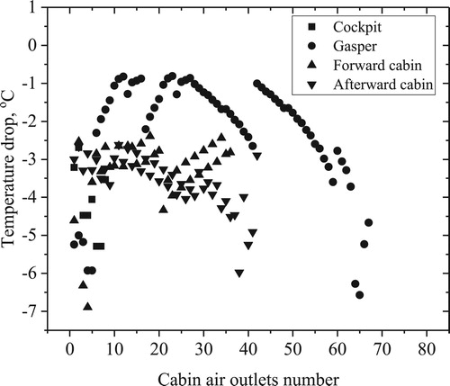
As stated in Section 2, to achieve the rapid cooling or warming of the air conditioning system on an extremely hot or cold day in ground conditions, there are severe demands on the insulation performance of the air distribution pipelines. As shown in Table 1, in the cabin temperature pulling-down process, the air temperature rise from the mix manifold outlet to the branch outlets should not exceed 3°C (hot day), while in the pulling-up process the air temperature drop through the pipeline should not exceed −7°C (cold day). The thermal insulation performance is mainly affected by the thickness and material thermal conductivity of the insulation layer of the pipeline. The diameters and internal air velocity of the pipeline are additional factors that affect the air temperature change along the pipeline. The 1D simulation models built in Section 3.2 can be used to calculate the thickness and thermal conductivity of the insulation layer which meet the design requirements, and can also be used to evaluate whether the existing insulation layer design meets the requirements of the objective temperature rise or temperature drop. As shown in Figures 10 and 11, the system insulation design has been evaluated so that the air temperature changes from the mix manifold to each branch outlet point are within the limitation requirements for all subsystems.

Figure 10. Temperature rise results in hot day conditions.

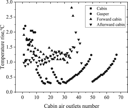
Figure 11. Temperature drop results in cold day conditions.

3.5. Flow distribution based on 1D analysis

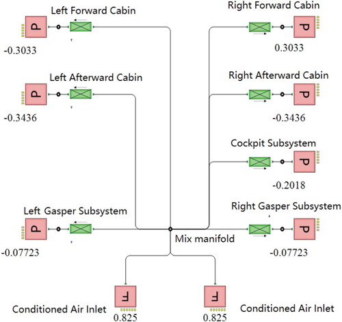
In the 1D simulation model, the mixer is assumed to be a node with energy and mass conservation. The flow source component model is used to set the total air flow mass into the mix manifold with the value of 0.825 kg/s. Pressure source components are used to set the outlet boundary with the value of 101,325 Pa. The pressure drop versus flow characteristics of each subsystem, which has already been obtained as shown in Figure 7, is modeled by discrete loss components. With this 1D fluid system model, the flow distribution result from the mix manifold to each subsystem can be calculated quickly, as shown in Figure 12.

Figure 12. Mix manifold system one-dimensional model (kg/s).

4. Flow distribution analysis of mix manifold based on CFD

4.1. Computational domain and grids

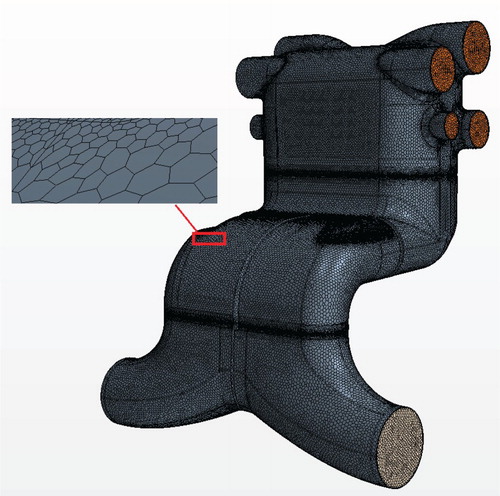
The computational domain of the mix manifold considered in the present study is shown in Figure 13. There are two fluid inlets with diameter 0.225 m to provide refrigerated air to the mix manifold, and seven fluid outlets directly connected to the air distribution system pipelines to supply conditioned air to different subsystems of the cabin (the diameter of the outlet connected to the left forward and right forward subsystem is 0.146 m, to the left and right afterward subsystem is 0.158 m, to the left and right gasper subsystem is 0.09 m, and to the cockpit subsystem is 0.102 m). The total calculation domain volume is 0.28 m³.

Figure 13. Schematic of the mix manifold and its computational domain.

The analysis involved the use of a commercial CFD code, STAR-CCM+. The surface-wrapping function of this software was used to obtain the inside fluid volume. Polyhedral meshes are used to fill the complex volume geometry, as shown in Figure 14. The polyhedral cell has more faces, which means that it also has more neighbors than traditional cell types such as hexahedral and tetrahedral meshes. Each polyhedral cell has an average of 12 or 14 neighbors. The information propagates much more quickly through a polyhedral mesh, ultimately leading to an increased rate of convergence. To avoid the influence of grid number on the calculation results, grid-independent verification is performed to verify the influence of different grid numbers. The model is divided into three different numbers of meshes: 1,131,739, 1,300,465 and 1,637,986. The results show that the change in grid number has little effect on the calculation results, and the number of grids is selected as 1,131,739 to save computing time.

Figure 14. Computational mesh of the mix manifold.

4.2. Boundary conditions

The inlet boundary condition of the calculation domain is set with a mass flow rate of 0.85 kg/s and the outlet boundary condition is the pressure jump. The pressure jump boundaries are described as curves of pressure drop versus mass flow rate. In this calculation, pressure jump boundary curves have already been obtained (see Figure 7). The whole mixer surface is covered with an insulation layer (thickness 10 mm and thermal conductivity $\text{0}\text{.04 w}/(\text{m}\cdot \text{k})$), which is converted into a convective heat transfer boundary in this calculation.

4.3. Solution method and control

The present computational analyses were performed with STAR-CCM+ version 13. The working fluid used in this calculation is air. The realizable two-layer k-epsilon model was chosen for modeling turbulence. The discrete equations of each variable were iterated by the semi-implicit method for pressure-linked equations (SIMPLE) algorithm, and all solutions were considered to be fully converged when the sum of residuals was below 10⁻⁵.

4.4. Results and discussion

4.2.1. CFD analysis results of mix manifold

As the pressure jump boundaries are set to the outlets of the mixer, the air entering the mixer will be distributed to each subsystem in a certain proportion owing to the different flow resistance at each outlet. As can be seen from the streamline of Figure 15, the two outlets connected to the afterward cabin pipelines have the largest proportion of flow distribution, while the values for cockpit and individual ventilation are relatively small.

Figure 15. Streamline of velocity magnitude by computational fluid dynamics (CFD) simulation.

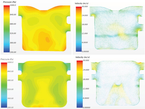
As a result of the different flow resistance values of the subsystem pipelines, which have been set as the pressure jump outlet boundary in the CFD model, the static pressure and velocity distribution near the outlet area are different, as shown by the pressure scalar field in Figure 16, which results in different air mass flow rates into the different subsystems. As can be seen from the structure of the mix manifold, the outlets are not completely symmetrical (three outlets on one side and four outlets on the other), leading to slight differences in the pressure and velocity at the outlets, even if the flow resistance values at the outlets are the same (such as the subsystems for the left and right sides). As a result, the flow distributions of the left and right side subsystems will also be different, and this is not considered in the 1D system simulation.

Figure 16. Pressure scalar field and velocity vectors for the internal section of the mix manifold by computational fluid dynamics (CFD) simulation.

4.2.2. Comparison of 1D method and CFD method

The 3D CFD model contains the complete internal structure of the mix manifold. Therefore, the influence of the internal structure of the mix manifold on flow distribution performance can be taken into account by this 3D model. Comparative analysis is carried out based on the same boundary conditions with the 1D and 3D models. The comparison results in Table 2 show that for the mix manifold model in this study, the calculation deviation of the mass flow rate for each subsystem using 1D and 3D simulation methods is from −0.95% to 7.24%. The right gasper subsystem has the largest deviation, at 7.24%, and the afterward cabin subsystem has the minimum deviation, at 0.95%. This difference is caused by the influence of the internal structure of the mix manifold. Different internal structure designs of the mix manifold will have different impacts on the inside flow of the mixer, which will affect the results of the flow distribution of the mix manifold; however, these impacts are neglected in the 1D simulation.

Table 2. Comparison between one-dimensional (1D) design results and three-dimensional computational fluid dynamics (CFD) design results.

Subsystem	Design objective (kg/s)	CFD analysis result (kg/s)	1D analysis result (kg/s)	Relative error (%)
Cockpit	0.2	0.1957	0.202	3.22
Forward cabin (left)	0.3	0.3214	0.303	−5.72
Forward cabin (right)	0.3	0.3157	0.303	−4.02
Afterward cabin (left)	0.35	0.3473	0.344	−0.95
Afterward cabin (right)	0.35	0.3473	0.344	−0.95
Gasper system (left)	0.075	0.0734	0.077	4.90
Gasper system (right)	0.075	0.0718	0.077	7.24

5. Conclusion

A design method applicable to complex multi-element cabin air distribution systems is developed based on 1D and 3D computational thermal fluid analysis. A 1D fluid subsystem model is built to evaluate the distribution uniformity and thermal insulation performance of the subsystem pipeline, and these 1D models are also used to calculate the P-Q characteristics of the subsystems, which are input boundary conditions used to analyze the distribution performance of the mix manifold. The 1D and 3D models of the mix manifold system are established and comparative analysis is conducted under the same boundary conditions. The comparison results show that the internal structure of the mix manifold will affect its flow distribution to the subsystems, and more than 7% deviation of the outlet mass flow rate results when using these two methods in this comparative study. The method presented in this study is developed based on the air distribution pipeline system of large-scale aircraft, and can also be used for the analysis and design of other similar pipeline systems.

The current research focuses on an efficient 1D and 3D engineering CFD method for the design and performance evaluation of complex air pipeline systems in large-scale aircraft. This work does not take into account the influence of cockpit temperature control processes on pipeline flow distribution, which also affect the flow field and temperature field of the aircraft cabin, and further impact the thermal comfort of the cockpit. Future work will focus on designing and optimizing the cabin flow and temperature field based on the comprehensive influence of the cockpit temperature control processes on the pipeline flow distribution and the cabin flow field.

Disclosure statement

No potential conflict of interest was reported by the author(s).

References

- Akbarian, E., Najafi, B., Jafari, M., Ardabili, S., Shamshirband, S., & Chou, K. (2018). Experimental and computational fluid dynamics-based numerical simulation of using natural gas in a dual-fueled diesel engine. Engineering Applications of Computational Fluid Mechanics, 12(1), 517–534. doi: 10.1080/19942060.2018.1472670
- Cao, X., Liu, J., Pei, J., Zhang, Y., Li, J., & Zhu, X. (2014). 2D-PIV measurement of aircraft cabin air distribution with a high spatial resolution. Building and Environment, 82, 9–19. doi: 10.1016/j.buildenv.2014.07.027
- China Civil Aviation Regulations, Part 25 Airworthiness Standards: Transport Category Airplanes§25.831 Ventilation (2011).
- Eero-Matti, S., & Holopainen, R. (2008). A PQ-formulation for ventilation duct system flow analyses. International Journal of Ventilation, 7(3), 251–265. doi: 10.1080/14733315.2008.11683816
- Li, C., Ji, C., Shi, M., & Sun, Q. (2019). Influence of rotor–stator component partition structure on the aerodynamic performance of centrifugal compressors. Engineering Applications of Computational Fluid Mechanics, 13(1), 1080–1094. doi: 10.1080/19942060.2019.1669075
- Miller, D. S. (1984). Internal flow systems. BHRA Fluid Engineering Series, vol. 5, Cranfield.
- Mou, B., He, B., Zhao, D., & Chau, K. (2017). Numerical simulation of the effects of building dimensional variation on wind pressure distribution. Engineering Applications of Computational Fluid Mechanics, 11(1), 293–309. doi: 10.1080/19942060.2017.1281845
- Ng, H. W., & Tan, F. L. (2009). Simulation of fuel behaviour during aircraft in-flight refueling. Aircraft Engineering and Aerospace Technology, 81(2), 99–105. doi: 10.1108/00022660910941785
- Pang, L., Xu, J., Fang, L., Gong, M., Zhang, H., & Zhang, Y. (2013). Evaluation of an improved air distribution system for aircraft cabin. Building and Environment, 59(59), 145–152. doi: 10.1016/j.buildenv.2012.08.015
- Park, J., Park, S., & Lee, D. K. (2016). CFD modelling of ventilation ducts for improvement of air quality in closed mines. Geosystem Engineering, 19, 177–187. doi: 10.1080/12269328.2016.1164090
- Poussou, S. B., Mazumdar, S., Plesniak, M. W., Sojka, P. E., & Chen, Q. (2010). Flow and contaminant transport in an airliner cabin induced by a moving body: Model experiments and cfd predictions. Atmospheric Environment, 44(24), 2830–2839. doi: 10.1016/j.atmosenv.2010.04.053
- Ramezanizadeh, M., Mohammad, A., Mohammad, H., & Chau, K. (2019). Experimental and numerical analysis of a nanofluidic thermosyphon heat exchanger. Engineering Applications of Computational Fluid Mechanics, 13(1), 40–47. doi: 10.1080/19942060.2018.1518272
- Shayne, Z., & Mentor Graphics. (2009). Computer simulation of an aircraft environmental control system. Retrieved from Mentor website: https://www.mentor.com/products/mechanical/resources/overview/computer-simulation-of-an-aircraft-environmental-control-system-b733ac00-a018-44d0-b188-fedd0b56065c
- Shi, H., Jiang, Y., Liu, Z., Kang, N., Yu, L., & Liu, C. (2013). Simulation of bleed air behavior during aircraft in flight based on flowmaster. Transactions of Nanjing University of Aeronautics and Astronautics, 30(2), 132–138. doi: 10.3969/j.issn.1005-1120.2013.02.004
- Society of Automotive Engineers. (2012). Air conditioning systems for subsonic airplanes. (SAE Publication No. ARP85F). Retrieved from https://www.sae.org/standards/content/arp85f/
- Swamee, P. K., & Jain, A. K. (1976). Explicit equations for pipe-flow problems. Journal of the Hydraulics Division, 102(5), 657–664. Retrieved from https://www.researchgate.net/publication/280018838_Explicit_eqations_for_pipe-flow_problems
- Tibor, K., Lawrence, C., & John, M. (2013). A new automotive air conditioning system simulation tool developed in matlab/simulink. SAE International Journal of Passenger Cars – Mechanical Systems, 6(2), 826–840. doi: 10.4271/2013-01-0850
- Tu, Y., & Lin, G. P. (2011). Dynamic simulation of aircraft environmental control system based on flowmaster. Journal of Aircraft, 48(6), 2031–2041. doi: 10.2514/1.C031433
- You, R., Chen, J., Shi, Z., Liu, W., Lin, C. H., Wei, D., & Chen, Q. (2016). Experimental and numerical study of airflow distribution in an aircraft cabin mock-up with a gasper on. Journal of Building Performance Simulation, 9, 555–566. doi: 10.1080/19401493.2015.1126762
- Zhang, T., & Chen, Q. (2007). Novel air distribution systems for commercial aircraft cabins. Building and Environment, 42(4), 1675–1684. doi: 10.1016/j.buildenv.2006.02.014
- Zítek, P., Vyhlídal, T., Simeunović, G., Nováková, L., & Čížek, J. (2010). Novel personalized and humidified air supply for airliner passengers. Building and Environment, 45(11), 2345–2353. doi: 10.1016/j.buildenv.2010.04.005