Numerical simulation of flow past a triangular prism with fluid–structure interaction

Abstract

Fluid flows around a pointed object, e.g. the flow around a triangular prism, are often encountered. In this study, numerical simulation of the flow around a triangular prism was carried out using COMSOL Multiphysics® software. Two cases were considered: the entire area of the triangular prism is fixed; and only the center is fixed. The first case is divided into three different flow models according to the flow state: the separation bubble model, the edge separation model and the attached flow model. The effects of different flow models on the lift coefficient, drag coefficient and Strouhal number were discussed from the perspective of fluid flow. For the second case, the triangular prism periodically rotates while the vortices are separated from the surface. It was found that a stable rotation stage exists after a certain period of time for prisms with different initial positions. The lift and drag coefficients of the triangular prism satisfy the jagged and sinusoidal variation.

KEYWORDS:

• Flow
• triangular prism
• fluid–structure interaction
• fixed constraint
• drag force
• flow–particle interaction

1. Introduction

In the thermodynamic cycle of nuclear power, nuclear fuel fissures in the reactor and generates a large amount of heat. The heat is taken out of the reactor by the coolant (e.g. carbon dioxide, helium or high-temperature sodium) (Sorokin, Alexeev, Kuzina, & Konovalov, 2017). Coolant flows around many objects throughout the thermal cycle. The problem of flow around the objects is one of the classical problems in fluid mechanics (Graf & Yulistiyanto, 1998). Under certain conditions, the boundary layer is separated from the surface of the object, which forms the wake region (Mustto & Bodstein, 2011). At lower values of Reynolds number (Re), this wake region is stably enclosed between the separated streamlines of the free stream (Camarri, Salvetti, & Buresti, 2006). However, with the increase in Re, the phenomenon of alternative shedding of vortices may occur in the wake region.

Many scholars have studied the flow around the cylinder in various ways. For example, the problems of flow around oscillating cylinders, rotating cylinders, variable cylinders, multi-cylinders and vortex detachment, oscillation and wave motion have been studied in depth (Huang & Ying, 2007; Ikeda, Harada, & Tokoi, 1980; Kakuda, Miura, & Tosaka, 2006; Pralits, Luca, & Flavio, 2010; Rival, Kriegseis, Schaub, Widmann, & Tropea, 2014; Sumner, Hemingson, Deutscher, & Barth, 2009; Yan, Zhou, & Jiahuang, 2013). A large number of numerical simulations has also been completed (Ghalandari, Mirzadeh Koohshahi, Mohamadian, Shamshirband, & Chau, 2019; Mosavi, Shamshirband, Salwana, Chau, & Tah, 2019; Ramezanizadeh, Alhuyi Nazari, Ahmadi, & Chau, 2019), mainly focusing on the development of the flow around the object. Even though the existing research publications have rigorously demonstrated various distinctions of flow over circular and square cylinders, the scenario with respect to triangular structures seems to have been less explored (Hines, Thompson, & Lien, 2009; Mustto & Bodstein, 2011; Prasath et al., 2014). There is often a phenomenon in which the fluid flows around a pointed object in the thermal system of nuclear power plants or other engineering applications, which can be regarded as the model of the flow around a triangular prism. Triangular prism flow is an emerging topic in the study of flow. The problem of flow around the triangular prism based on fluid–solid coupling includes the collision of fluid and solid, the separation of fluid, the generation and detachment of the vortex, and the change of solid structure. Because its cross-sectional shape is triangular, the flow field separation has special characteristics, especially in reducing flow resistance.

Camarri et al. (2006) numerically studied the flow around a triangular prism with a moderate aspect ratio placed vertically on a plane using the large-eddy simulation approach. The results were compared with experimental data to obtain clues on the physical origin of the velocity fluctuations inside and around the wake. Eiamsa-Ard, Sripattanapipat, and Promvonge (2012) numerically investigated heat transfer and flow behavior in a channel fitted with a transverse triangular prism pair in the turbulent flow regime for Reynolds number ranging from 10,000 to 50,000. Saha (2013) used the Direct Numerical Simulation (DNS) to solve the flow problem and simulate the flow past a finite length square cylinder at a Reynolds number of 250. Saha found that different inflow directions cause changes in the vortex detachment, and also affect the lift, drag and frequency of vortex detachment. Lee and Lim (2001) analyzed the flow characteristics around a two-dimensional triangular-shaped prism located behind a porous wind fence by using the numerical method which is based on the finite volume method with the QUICK scheme. Prasath et al. (2014) determined the effects of aspect ratio and Reynolds number on the drag force coefficient (C_D), as characterized for two different geometric orientations of the prism (base or apex facing the flow). Agrwal, Dutta, and Gandhi (2016) completed an experimental study on the flow around a triangular prism under the influence of a sharp angle. The results obtained in the present work are Strouhal number, drag coefficient, time-averaged and instantaneous velocity field, and statistical quantities such as turbulence intensity and shear stress. Bao, Zhou, and Zhao (2010) studied the characteristics of shedding vortices at different angles by numerical calculation. It was pointed out that the shedding vortices formed leeward of the apex were quite different from those formed upwind of the apex.

In this paper, numerical simulation of the flow around the triangular prism with different fixed types was carried out using COMSOL Multiphysics® software. First, the flow around the whole-area fixed triangular prism was simulated and the influence of the relative positional relationship of the triangular prism and the fluid was analyzed. Then, we simulated the flow around the triangular prism in which the central region of the prism is fixed, and discussed the effect of the initial position on the rotation of the triangular prism.

2. Arbitrary Lagrange–Euler (ALE) description

2.1. Introduction to three descriptive methods

The main characteristic of a fluid–solid coupling problem is the interaction between fluid and solid (Yu, Wang, & Li, 2009). The fluid leads to solid deformation, vibration, rotation and other changes, and the changed solid affects the velocity and pressure of the flow field. When solving the fluid–structure coupling problem, one needs to solve the fluid governing equation (to obtain the velocity and pressure of the node) and the solid governing equation (to obtain the displacement of the node). In the process of studying solid mechanics, the Lagrangian description (Binder, Hirokawa, & Windhorst, 2009) is generally chosen because it is more concerned with the changes in the solid itself. In the process of using the Lagrangian description, the mesh node and the object structure always coincide in the whole motion process. There is no relative motion between the object structure and the mesh node, so it is easy to track the motion of the solid and accurately describe the deformation and operation of the solid. Euler description is generally used for fluids. Its research goal is to locate the nodes in space. The mesh always keeps the initial state during the whole calculation process, which can accurately describe the changes in fluid particle motion.

When solving the fluid–solid coupling problem, it is necessary to transfer the interaction force between the fluid and solid boundary, so two different descriptions are needed to transform each other. The COMSOL software mainly uses ALE descriptions to solve this problem (Jafari & Okutucu-Özyurt, 2016).

2.2. Definition of mesh displacement, velocity and acceleration in three descriptive methods

Euler’s description is commonly used in fluid mechanics. The Eulerian coordinate system is also called the spatial coordinate system. It can accurately describe the spatial position of the nodes without changing the deformation or motion of the solid. Lagrangian descriptions are used for solid analysis. Lagrange’s description mainly focuses on the solid structure, and its coordinate system can be defined as a material coordinate system. When the object deforms or moves, the material coordinate system changes accordingly (Mcintyre, 1980). It can be prepared to describe the structural deformation and motion of solids. The coordinate system of the ALE description method is neither fixed in space like the Eulerian coordinate system nor fixed in solid material like the Lagrangian coordinate system (Dang & Meschke, 2014). The ALE coordinate system can move arbitrarily, which is the unique advantage of the ALE description method.

Define as the space coordinate system, $X$ as the material coordinate system and $\chi$ as the ALE coordinate system (Figure 1).

Figure 1. Concept diagrams of Lagrange, Euler and arbitrary Lagrange–Euler (ALE) coordinate systems.

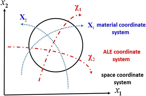
The ALE coordinate system is defined as the initial position of the spatial coordinate system. Because of the deformation of the solid, the ALE coordinate system can move along with it. The difference between the final position and the initial displacement of the ALE coordinate system in period $t$ is defined as the material displacement $w(X,t)$. The displacement and moving speed of meshes in ALE coordinates are defined as follows: (1) $\begin{array}{rl}\chi & =\phi (\chi ,0)\end{array}$(1) (2) $\begin{array}{rl}\Delta \chi & =\phi (\chi ,t)-\phi (\chi ,0)=x-\chi \end{array}$(2) (3) $\begin{array}{rl}w(\chi ,t)& =\frac{\mathrm{\partial }\left(\phi \right(\chi ,t)-\phi (\chi ,0\left)\right)}{\mathrm{\partial }t}\\ & =\frac{\mathrm{\partial }x(\chi ,t)}{\mathrm{\partial }t}-\frac{\mathrm{\partial }\chi }{\mathrm{\partial }t}=\frac{\mathrm{\partial }x(\chi ,t)}{\mathrm{\partial }t}=\frac{\mathrm{\partial }x}{\mathrm{\partial }t}\end{array}$(3) where $\phi (\chi ,0)$ is the initial position of the node in the ALE coordinate system, $\phi (\chi ,t)$ is the final position, $\Delta \chi$ is the displacement of the node, and $w(\chi ,t)$ is the velocity of the node.

In the same way, the displacement and moving speed of meshes in Lagrangian coordinates are defined as follows: (4) $\begin{array}{rl}X& =\varphi (X,0)\end{array}$(4) (5) $\begin{array}{rl}\Delta X& =\varphi (X,t)-\varphi (X,0)=x-X\end{array}$(5) (6) $\begin{array}{rl}u(X,t)& =\frac{\mathrm{\partial }\left(\varphi \right(X,t)-\varphi (X,0\left)\right)}{\mathrm{\partial }t}\\ & =\frac{\mathrm{\partial }x(X,t)}{\mathrm{\partial }t}-\frac{\mathrm{\partial }X}{\mathrm{\partial }t}=\frac{\mathrm{\partial }x(X,t)}{\mathrm{\partial }t}=\frac{\mathrm{\partial }X}{\mathrm{\partial }t}\end{array}$(6) where $\varphi (X,0)$ is the initial position of the node in the Lagrange coordinate system, $\varphi (X,t)$ is the final position, $\Delta X$ is the displacement of the node, and $u(X,t)$ is the velocity of the node.

The transformation relations between Lagrange, Eulerian and ALE coordinates are given. The same function $f$ is expressed in Lagrange, Euler and ALE coordinates as $f(X,t)$, $f(x,t)$ and $f(\chi ,t)$, respectively. The transformation relations of the three coordinate systems are as follows: (7) $\begin{array}{rl}{x}_i& ={\varphi }_i(X,t)={\phi }_i(\chi ,t)\end{array}$(7) (8) $\begin{array}{rl}\frac{df}{dt}& =\underset{\text{Derivatives in Lagrange coordinates}}{\underbrace{{\left.\frac{\mathrm{\partial }f(X,t)}{\mathrm{\partial }t}\right|}_X}}+\frac{\mathrm{\partial }f(X,t)}{\mathrm{\partial }X}\underset{=0}{\underbrace{{\left.\frac{\mathrm{\partial }X}{\mathrm{\partial }t}\right|}_X}}\\ & =f_{t\left[X\right]}\end{array}$(8) (9) $\begin{array}{rl}\frac{df}{dt}& =\underset{\text{Derivatives in Euler coordinates}}{\underbrace{{\left.\frac{\mathrm{\partial }f(x,t)}{\mathrm{\partial }t}\right|}_x}}+\frac{\mathrm{\partial }f(x,t)}{\mathrm{\partial }x}\underset{=w}{\underbrace{{\left.\frac{\mathrm{\partial }x}{\mathrm{\partial }t}\right|}_X}}\\ & =f_{t\left[x\right]}+v\cdot {\mathrm{\nabla }}_{x}f\end{array}$(9) (10) $\begin{array}{rl}\frac{df}{dt}& =\underset{\text{Derivatives in ALE coordinates}}{\underbrace{{\left.\frac{\mathrm{\partial }f(\chi ,t)}{\mathrm{\partial }t}\right|}_{\chi }}}+{\left.\frac{\mathrm{\partial }f(\chi ,t)}{\mathrm{\partial }\chi }\frac{\mathrm{\partial }\chi }{\mathrm{\partial }t}\right|}_X\\ & ={\left.\frac{\mathrm{\partial }f(\chi ,t)}{\mathrm{\partial }t}\right|}_{\chi }+{\left.\frac{\mathrm{\partial }f(\chi ,t)}{\mathrm{\partial }x}\frac{\mathrm{\partial }x(\chi ,t)}{\mathrm{\partial }\chi }\frac{\mathrm{\partial }\chi }{\mathrm{\partial }t}\right|}_X\\ & ={\left.\frac{\mathrm{\partial }f(\chi ,t)}{\mathrm{\partial }t}\right|}_{\chi }+\left[{\left.\frac{\mathrm{\partial }x}{\mathrm{\partial }t}\right|}_X-{\left.\frac{\mathrm{\partial }x}{\mathrm{\partial }t}\right|}_{\chi }\right]\cdot \frac{\mathrm{\partial }f(\chi ,t)}{\mathrm{\partial }x}\\ & =f_{t\left[\chi \right]}+(u-w)\cdot {\mathrm{\nabla }}_{x}f\end{array}$(10)

2.3. Fundamental governing equations in ALE

When using the COMSOL Multiphysics software to simulate the coupling flow around the cylinder, the built-in fluid–structure coupling module can be used (Münch, Ausoni, Braun, Farhat, & Avellan, 2010). Fluid–structure coupling modules involve governing equations for fluids, solids and fluid–solid coupling boundary conditions.

In the Cartesian coordinate system, the momentum equation and continuity equation for two-dimensional non-compressible viscous fluids are: (11) $\begin{array}{rl}\frac{\mathrm{\partial }{u}_x}{\mathrm{\partial }t}+u_x\frac{\mathrm{\partial }{u}_x}{\mathrm{\partial }x}+u_y\frac{\mathrm{\partial }{u}_x}{\mathrm{\partial }y}& =-\frac{1}{\rho }\frac{\mathrm{\partial }p}{\mathrm{\partial }x}+\upsilon (\frac{{\mathrm{\partial }}^2{u}_x}{\mathrm{\partial }{x}^2}+\frac{{\mathrm{\partial }}^2{u}_x}{\mathrm{\partial }{y}^2})\end{array}$(11) (12) $\begin{array}{rl}\frac{\mathrm{\partial }{u}_y}{\mathrm{\partial }t}+u_x\frac{\mathrm{\partial }{u}_y}{\mathrm{\partial }x}+u_y\frac{\mathrm{\partial }{u}_y}{\mathrm{\partial }y}& =-\frac{1}{\rho }\frac{\mathrm{\partial }p}{\mathrm{\partial }y}+\upsilon (\frac{{\mathrm{\partial }}^2{u}_x}{\mathrm{\partial }{x}^2}+\frac{{\mathrm{\partial }}^2{u}_x}{\mathrm{\partial }{y}^2})\end{array}$(12) (13) $\begin{array}{rl}\frac{\mathrm{\partial }\rho }{\mathrm{\partial }t}+\frac{\mathrm{\partial }\left(\rho u_x\right)}{\mathrm{\partial }x}+\frac{\mathrm{\partial }\left(\rho u_y\right)}{\mathrm{\partial }y}& =0\end{array}$(13) where $\upsilon$ is the kinematic viscosity of the fluid, its magnitude is equal to the ratio of the dynamic viscosity of the fluid to the density of the fluid, and $u_x$ and $u_y$ are the fluid velocity components in the $x$direction and $y$ direction, respectively.

In the ALE description method, the momentum equation of fluid can be expressed as: (14) $\frac{\mathrm{\partial }u}{\mathrm{\partial }t}+(v-w)\cdot \mathrm{\nabla }v+\mathrm{\nabla }\cdot {\sigma }^F-f^F=0$(14) where $\mathrm{\nabla }$ is the gradient operator, $v$ is fluid velocity, $w$ is grid velocity, $v-w$ is relative velocity, ${\sigma }^F$ is the fluid stress tensor, and $f^F$ is fluid mass force.

The force generated by the fluid is (Yue, Liu, Liu, Min, & Dong, 2018): (15) ${\sigma }_f=-n\cdot (-pI+\mu (\mathrm{\nabla }u+(\mathrm{\nabla }u{)}^T\left)\right)$(15) where ${\sigma }_f$ is the sum of the viscous forces of pressure and fluid, $-pI$ is the static pressure generated by the fluid, $I$ is the unit diagonal matrix, $n$ is the normal vector of the boundary, $\mu$ is the kinematic viscosity of the fluid, and $\mu (\mathrm{\nabla }u+(\mathrm{\nabla }u{)}^T)$ is the flow stress of the fluid.

The governing equation for solids is (Hank, Gavrilyuk, Favrie, & Massoni, 2017): (16) $\rho \frac{{\mathrm{\partial }}^2{u}_{\text{solid}}}{{\mathrm{\partial }}^{2}t}=\mathrm{\nabla }\cdot \sigma +F_v$(16) where $\rho$is the density of the solid, $u_{\text{solid}}$ is the displacement of the solid, $\sigma$ is the stress on the cylinder, and $F_v$ is the volumetric force.

The solid and fluid contact each other at the boundary. According to the relevant laws of physics, the velocity and stress of the fluid and solid at the coupling boundary should be equal and opposite (Ng, Min, & Gibou, 2009): (17) $\left\{\begin{array}{l}{\sigma }_s\cdot n={\sigma }_f\cdot n\\ u_f=u_s=w\end{array}\right.$(17) where ${\sigma }_s$ is the stress on the solid, ${\sigma }_f$ is the stress on the fluid, $u_s$ is the velocity of the solid boundary node, $u_f$ is the velocity of the node at the fluid boundary, and n is the boundary normal vector.

3. Numerical model and conditions

The computational area is shown in Figure 2. The flow field is selected as a rectangle, and the lower left corner of the rectangle is taken as the origin of the coordinates. The two-dimensional cross-section of the triangular prism is an equilateral triangle. The center point coordinates are (15 mm, 15 mm), the radius of the circumscribed circle is 1 mm and the characteristic length is 2 mm. The laminar flow model is selected as the flow model in this paper. The flow rate inlet is set at the left boundary of the flow field and the pressure outlet is set at the right boundary. In this simulation, the fluid material is air and the solid material is steel. Their physical properties are shown in Tables 1 and 2.

Figure 2. Computational area and mesh division of flow around the triangular prism.

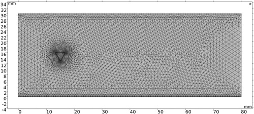
Table 1. Physical parameters of fluids.

Fluid material	Density (kg/m^3)	Dynamic viscosity (Pa·s)
Air	1.293	$17.09\times {10}^{-6}$

Table 2. Physical parameters of solids.

Solid material	Density (kg/m^3)	Modulus of elasticity (GPa)	Poisson ratio	Object shape
Steel	7085	210	0.269	Equilateral triangle

Using the built-in meshing function of COMSOL Multiphysics, the triangle mesh size of the entire region is set to the refinement standard of fluid dynamics. To simulate the vortex detachment situation more accurately, mesh refinements are performed in the region of the flow field where vortex streets may be generated (Murayama, Nakahashi, & Sawada, 2001). By performing grid independence verification, the overall computational area is divided into 3844 grid vertices and 7289 grid elements under the premise of taking into account the accuracy and time of computation. The average skewness of the grid is 0.829.

4. Analysis of flow around the fixed entire area of the triangular prism

4.1. Definition of the angle between the triangular prism and the fluid

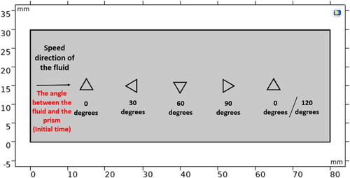
In the thermodynamic cycle of a nuclear power plant, the incoming fluid may flow through the triangular prism from any direction. Owing to the presence of the corners, the relative positional relationship between the triangular prism and the fluid affects the flow field distribution. This article only discusses the problem of the flow around a triangular prism in four different locations. Because of the symmetry of the equilateral triangle, the equilateral triangle returns to its original position after rotating 120° around the center. To analyze the flow around a triangle more accurately, the rotation degree of an equilateral triangle is set at 30° per difference as a calculation condition. As shown in Figure 3, the four cases are defined as follows: the angle between the fluid and the triangular prism is 0°, 30°, 60° and 90°.

Figure 3. Schematic diagram of the flow field at different angles between the triangular prism and the fluid.

4.2. Classification of flow models

The different angles between the fluid and the prism make the flow very complicated. Figure 4 is a schematic diagram of the flow field of the triangular prism at four different angles.

Figure 4. Schematic diagram of the flow field at different angles between the triangular prism and the flow velocity: (a) angle = 0°; (b) angle = 30°; (c) angle = 60°; (d) angle = 90°.

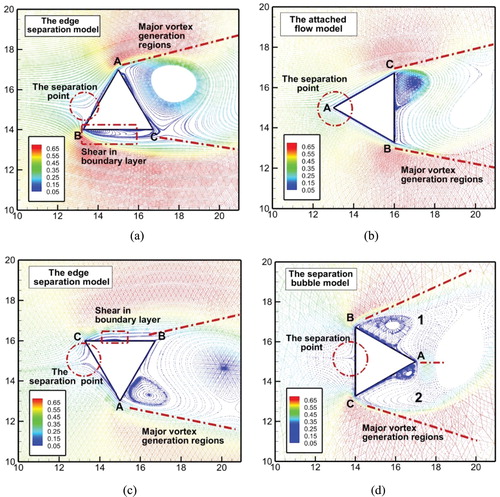
When the angle between the triangular prism and the fluid is 0° or 60°, this flow state is defined as the edge separation model. The edge separation model is discussed and illustrated by taking the case where the angle between the prism and the fluid is 0° as an example. The flow diagram is shown in Figure 4(a). The fluid is separated by directly impacting the wall of the prism. The position of the fluid separation point is near the end point B of side AB. The separated fluid moves along the wall until it reaches the corner of the prism. When part of the fluid after separation moves to the corner of the triangular prism far from the separation point (point A), the fluid moves far from the wall of the triangular prism. When the other fluid moves to the corner of the triangular prism near the separation point (point B), the fluid continues to move along the wall (edge BC) and shears occurs in the boundary layer. This part of the fluid eventually moves away from the wall at point C. The major vortex generation region is formed in the right side region of the triangular prism. The characteristic of this flow model is that one part of the fluid moves along both sides of the wall and the other part is directly away from the wall after separation.

When the angle between the triangular prism and the fluid is 30°, the flow state is defined as the attached flow model. The fluid is separated from point A and the separated fluid flows along the two walls of the triangular prism (edge AC and edge AB). The major vortex generation region is formed in the right side region of the triangular prism. The characteristic of this flow model is that the fluid moves along both sides of the wall.

When the angle between the triangular prism and the fluid is 90°, this flow state is defined as the separation bubble model. The fluid is separated into two parts at the center of the triangular prism wall (the midpoint of edge BC). The separated fluid moves along the wall (edge BC) until it reaches the corner of the prism (point B and point C). After that, the fluid moves away from the wall. The characteristic of this flow model is that fluid separates from the walls directly and the area where the vortex breaks away is larger. The vortices are formed alternately near the walls on both sides of the prism (regions 1 and 2 in Figure 4d).

Table 3 summarizes the characteristics of the three different flow models mentioned above.

Table 3. Classification and characteristics of different flow models.

Angle between triangular prism and fluid (°)	Flow model	Characteristics
0/60	Edge separation model	One part moves along the wall and the other part is far away from it
30	Attached flow model	The separated fluid moves along the wall
90	Separation bubble model	The separated fluid moves far away from the wall

4.3. Influence of the angle between the triangular prism and the fluid on the lift and drag coefficients

In solving engineering problems, the dimensionless pressure coefficient is often used to define the pressure at any point of the cylinder (Meng et al., 2018). The definition of the pressure coefficient is (18) $C_p=\frac{p_w-p_{\mathrm{\infty }}}{1/2\rho v_{\mathrm{\infty }}^2}$(18) where $C_p$ is the pressure coefficient, $p_w$ is the pressure on the wall of the cylinder, $p_{\mathrm{\infty }}$ is the fluid pressure at infinity, $\rho$ is the velocity of the fluid, and $v_{\mathrm{\infty }}$ is the velocity of the fluid at infinity.

In COMSOL, the pressure on the grid nodes with the prism boundary can be calculated directly. After obtaining the pressure coefficient of the solid boundary node using the data processing function in COMSOL, the lift coefficient and the drag coefficient can be obtained using the relationship between the pressure coefficient and the correlation coefficient (Hai, Zhong, & Yun, 2013): (19) $\begin{array}{rl}{C}_l& ={\oint }_c\left(C_p\right(s\left)/c\right)n_y\left(s\right)ds\\ C_d& ={\oint }_c\left(C_p\right(s\left)/c\right)n_x\left(s\right)ds\end{array}$(19) where $C_l$ is the lift coefficient, $C_d$ is the drag coefficient,; $C_p\left(s\right)$ is the pressure coefficient, $n_x\left(s\right)$ is the X-direction component of the normal vector, and $n_y\left(s\right)$ is the Y-direction component of the normal vector.

The Reynolds number of the fluid is equal to 150 and the flow state is laminar flow. The results of the simulation are collated. The lift and drag coefficients of the triangular prism at five different angles are obtained as shown in Figure 5.

Figure 5. Variation in drag and lift coefficient of the cylinder with time at different angles: (a) angle = 0°; (b) angle = 30°; (c) angle = 60°; (d) angle = 90°.

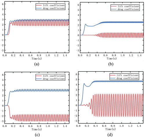
The lift and drag coefficients of the above four cases all fluctuated periodically with time, which also indicated that the vortex periodic detachment occurred in these four cases (Home & Lightstone, 2014). However, there are significant differences in the flow characteristics of the four cases. The amplitudes of the lift coefficient and the drag coefficient are different. This represents the magnitude of the force produced by the flow. The largest amplitude is 90° and the smallest amplitude is 60°. That is, the magnitude of the force in the separated bubble model is the largest and the attached flow model is the smallest.

Because the separated fluid moves far away from the wall, the vortices are formed alternately near the walls on both sides of the prism and the flow process is more asymmetrical. For this reason, the amplitude of the lift and drag coefficients of the split bubble model are maximum and the separated bubble model is the greatest. Similarly, because the fluid moves along the wall after separation in the attached flow model, it is more symmetrical during the movement of the fluid, and the amplitude of the lift and drag coefficients in the attached flow model is minimal and the magnitude of the force is the smallest.

In the edge separation model, one part moves along the wall and the other part is far away from it. It belongs to the transition state between the other two models, so the coefficient amplitude of this model is smaller than that of the separation bubble model and larger than the attached flow model.

By averaging the lift coefficient and the drag coefficient, the average drag and lift coefficients of the triangular prism during the flow can be obtained, as shown in Figure 6.

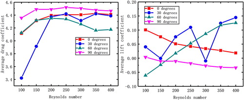
Figure 6. Variation in average drag and lift coefficients with the angle.

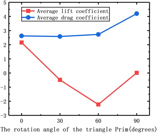
Under the same inflow conditions, the different angles of the triangular prism and the fluid directly affect the average lift and drag coefficient. When the angle between the triangular prism and the fluid is 30° and 90°, the lift coefficient is close to zero. In the attached flow model or the separation bubble model, the motion of fluid on the upper and lower walls of a prism is symmetrical, so the contribution of fluid to lift is very small. When the angle between the triangular prism and the fluid is 60°, the lift coefficient of the triangular prism is negative in the edge separation model. Finally, when the angle is 0°, the lift coefficient is positive. This proves that the initial positions of the prisms have a decisive influence on the pressure on the surface of the prisms.

As far as the drag coefficient is concerned, the separation bubble model has the largest drag coefficient. Because to the separated fluid moves far away from the wall, the flow process is more asymmetrical, with greater fluctuation, and it causes the drag coefficient to increase.

4.4. Influence of the angle between the triangular prism and the fluid on the Strouhal number

When the Reynolds number satisfies certain conditions, the boundary layer is separated from the surface of the object, which forms the periodically distributed vortex. Owing to the periodic detachment of the vortex, the object is subject to a periodic exciting force (Wang, Evans, & Jameson, 2017). When the natural frequency of the object is the same as or close to the frequency of the exciting force, the vibration of the object is intensified because of the enhanced coupling effect of the fluid and the solid (Suangga, Hidayat, Juliastuti, & Bontan, 2017). When the maximum amplitude exceeds a certain value, the structure of the object is irreversibly destroyed. Therefore, vortex detachment frequency in the flow around the triangular prism is of great significance for engineering problems.

In practical engineering problems, the Strouhal number is often used to reflect the speed of vortex separation: (20) $St=\frac{fd}{v}$(20) where $f$ is the detachment frequency of the vortex, $d$ is the characteristic length, and v is the flow velocity.

Because the periodic detachment of the vortex causes periodic changes in the lift and drag of the cylinder, the frequency of vortex detachment is the same as the lift and drag. In the field of mathematics and signal processing, the Fourier transform can be used to obtain the correspondence between the signal frequency and the amplitude. The frequency spectrum can be used to find the frequency of the periodic signal. Based on this method, the Fourier change of the lift coefficient and the drag coefficient can obtain the detachment frequency of the vortex. The related simulation data are summarized and sorted to obtain the relationship between the Strouhal number and the angle between the triangular prism and the fluid, as shown in Figure 7.

Figure 7. Variation in Strouhal number with the angle.

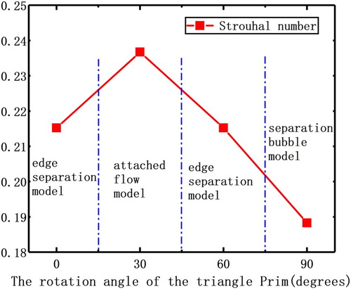
In the flow around the triangular prism, the attached flow model has the largest Strouhal number and the separation vortex has the smallest Strouhal number. In the attached flow model, the vortex generated on the right side of the triangular prism is not limited. The vortex can detach from the surface more easily and the time is the shortest. In the separation bubble model, two different major vortex generation regions are formed near the right side surface of the triangular prism. In this case, the generated vortex is restricted inevitably by the right side surface during the development process. The time required for the vortex to detach from the object is the longest, which means that the Strouhal number is the smallest. Unlike the separation bubble model, only a portion of the vortex in the generation region is restricted by the right side surface in the edge separation model. The other portion is not limited, which is similar to the attached flow model. Therefore, the Strouhal number of the edge separation model is between those of the attached flow model and the separated bubble model.

5. Analysis of flow around the triangular prism with a fixed centroid

The foregoing discussion is about the flow around the triangular prism when the entire area is fixed, but there may be another type, where the center of the triangular prism is fixed. Therefore, this section discusses the case in which the center of the triangle (the center of the triangular prism) is fixed. In this case, the triangular prism rotates because the fluid constantly impacts the edges and corners of a triangular prism. However, the initial positions of different prisms affect the whole process of the prism from stationary to stable rotation. Similarly to the previous work, the flow around the fixed triangular prism at four different initial positions is calculated and simulated in this paper.

During the rotation of the triangular prism, the vortex detachment still occurs, so the changes in lift and drag of the triangular prism are more complicated. The establishment of the model for this problem and the division of the mesh are similar to the previous one, and the fixed constraint is changed to the center of the triangular prism. One of the main features of COMSOL Multiphysics is that meshes can be automatically generated according to the actual situation. When the triangular prism rotates in the flow field, if the maximum distortion of the mesh element is less than 4, which means that the mesh deformation is serious at this time, COMSOL will redivide the mesh and continue to operate (Ibrahim, Ng, & Wong, 2011).

5.1. Analysis of the influence of initial position on flow around the triangular prism with fixed centroid

The initial position of the triangle affects the whole process from the beginning to the stability of the prism. This paper mainly calculates the lift and drag coefficients, and the rotation angle of the prism in the process. The effects of the fixed prism center on solids and fluids are obtained by analyzing the changes in these parameters.

The lift and drag coefficients can be obtained according to the Fourier change, similarly to the previous method. In the COMSOL software, one can set the domain point probe and record continuously the change in position (Das & Ray, 2017). Because the center of the prism is fixed, the moving trajectory of the apex in the triangular prism is circular. The rotation angle can be obtained using the following formula: (21) $\alpha =\frac{180l}{\pi r}$(21) where $l$ is the travel distance of the apex, r is the radius length of the circumferential circle of the triangle, and $\alpha$ is the rotation angle of the triangle.

In the following subsections, the flow around the prism in four different initial positions is discussed.

1. The angle between the initial position of the triangular prism and fluid is 0° or 60°

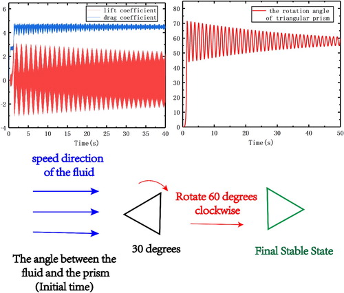
In this case, the lift and drag coefficients of the prism do not satisfy the sinusoidal variation, as in Figure 5 (the case where the entire area of the triangular prism is fixed). This is because the prism with a fixed center can rotate freely in the flow field. Figure 8 shows that the rotation of the prism tends to be stable after a certain period of time. The final average rotation angle is 30°, which proves that the prism finally rotates steadily near a certain position.

Figure 8. Schematic diagram of the lift and drag coefficients, variation in displacement with time, and sketch of rotation when Reynolds number = 150 and angle = 0°.

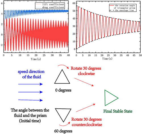
It can be seen that the prism is in a stable state of rotation, and its rotation angle changes with time to meet certain rules. We use MATLAB® software to obtain the envelope of the above rotation angle and the fitting results. The analytical expression of the fitting function is: $y=A1+A2\cdot e^{A3\cdot x}$

The results of envelope fitting of the rotation angle in the above two cases are as follows (Tables 4 and 5).

Table 4. Envelope fitting coefficient when the angle = 0°.

Reynolds number	A1	A2	A3
100	32.1347	24.8237	−0.0388
150	32.3213	24.3325	−0.0437
200	33.5051	23.6674	−0.0439
250	35.1392	22.1887	−0.0428
300	37.9361	19.7183	−0.0449
350	39.2351	18.9801	−0.0491
400	41.864	16.6869	−0.054

Table 5. Envelope fitting coefficient when the angle = 60°.

Reynolds number	A1	A2	A3
100	15.916	12.3024	−0.0371
150	15.9835	12.214	−0.0385
200	17.6612	10.7768	−0.034
250	21.4641	7.4191	−0.0466
300	24.864	4.4117	−0.0687
350	26.9842	2.5491	−0.1044
400	27.1508	2.5504	−0.1174

From the fitting results of the envelope above, it can be seen that the rotation rules of the two cases are similar on the whole, but the details are different. For example, with the increase in Reynolds number, the rotation rate of the prism increases and the rotation angle becomes more stable. In other words, with the increase in Reynolds number, the coefficient of A3 also decreases. However, the coefficient of A3 decreases more rapidly when the angle between the initial position of the prism and the fluid is 60° than when the angle is 0°. That is, the prism can reach the stable state more easily when the angle is 60° in the above two cases.

1. The angle between the initial position of the triangular prism and the fluid is 30°

In this case, lift and drag coefficients are similar to those in the previous case. However, the rotation of the prism has changed. In the initial stage of motion (< 5 s), the rotation angle of the prism quickly increases from 0° to about 70°. It finally stabilizes to about 60°. The prism reaches the stable state near the angle of 90° between the prism and the fluid, which is the same as in the previous case (Figure 9).

1. The angle between the initial position of the triangular prism and the fluid is 90°

Figure 9. Schematic diagram of the lift and drag coefficients, variation in displacement with time, and sketch of rotation when Reynolds number = 200 and angle = 30°.

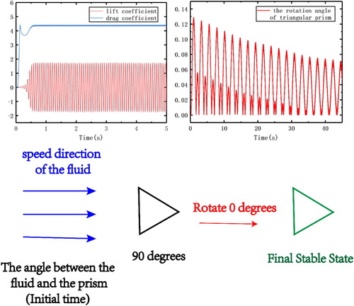
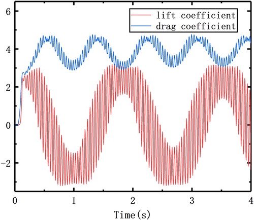
As shown in Figure 10, the lift and drag coefficients substantially satisfy the sinusoidal variation, because the degree of rotation of the triangular prism is very small in this case. Taking the apex of the triangular prism as the research object, the maximum rotation angle of the triangular prism is less than 0.5°, which is much smaller than in the previous two cases. In this case, the initial position is closest to the equilibrium state, so the flow of the fluid is the most stable and the degree of rotation is very small. This situation is similar to the flow around the triangular prism when the entire area is fixed.

Figure 10. Schematic diagram of the lift and drag coefficients, variation in displacement with time, and sketch of rotation when Reynolds number = 100 and angle = 90°.

5.2. Analysis of the steady state of triangular prism rotation

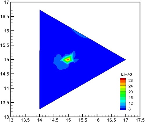
From the above analysis, it can be found that there is a stable rotational position in the flow around the fixed center triangular prism. Regardless of the initial position of the triangular prism, the triangular prism eventually rotates stably around this position owing to the force of the fluid. This stability is found in the vicinity of the 90° angle between the triangular prism and the fluid. This steady state is the result of the force balance of the triangular prism. On the one hand, the fluid gives a force to the triangular prism. On the other hand, because the triangular prism is fixed at the center, the rotation of the prism generates internal force, as shown in Figure 11.

Figure 11. Distribution of internal force on the prism.

5.3. Analysis of the influence of prism rotation on the lift and drag coefficients

For the three different initial positions of the triangular prism, the average lift and drag coefficients are obtained by averaging the lift and drag coefficients. The average lift and drag coefficient can comprehensively reflect the force of the triangular prism, which plays an important role in studying the influence of fluid on the object (Roohi, Zahiri, & Passandideh-Fard, 2013) (Figure 12).

Figure 12. Variation in average drag and lift coefficients with the angle.

With the increase in the inflow velocity, it can be found that the minimum fluctuation of the average lift and drag coefficient occurs when the angle between the initial position of the triangular prism and the fluid is 90°. At this time, the triangular prism does not rotate substantially and the lift and drag coefficients basically satisfy the sinusoidal variation. When there is the flow around a triangular prism of which the center is a fixed area, as in a nuclear power plant or in other engineering applications, the angle between the initial position of the triangular prism and the fluid should be set to 90°. In this case, the flow is the most stable, which is beneficial to improve the service life and ensure the safety of the object. In the other cases, the degree of rotation is greater and the fluctuations in the lift and drag coefficients are larger.

When the angle between the triangular prism and the fluid is 0°, 30° and 60°, the triangular prism undergoes a large degree of rotation. At the same time, periodic detachment of the vortex occurs. It can be seen from Figure 13 that the lift and drag coefficients of the triangular prism satisfy the rule of jagged and sinusoidal variation. The jagged variation is caused by the periodic detachment of the vortex, and the regularity of the sinusoidal variation is due to the periodic rotation of the triangular prism. The period of vortex detachment is much smaller than the rotation period of the triangular prism, so the lift and drag coefficients satisfy the rule of jagged variation locally, and the sinusoidal variation law is satisfied as a whole.

Figure 13. Partial enlarged view of lift and drag coefficients.

6. Conclusion

In the thermal system of nuclear power plants and other engineering applications, there is often a phenomenon in which the fluid flows around a pointed object. This can be regarded as a model of the flow around a triangular prism. From the point of view of the coupling of fluid and an object, the numerical simulation of the flow around the triangular prism was carried out using COMSOL Multiphysics software. The main conclusions are as follows.

The case where the entire triangular prism is fixed is divided into three models according to the flow state: the separation bubble model, the edge separation model and the attached flow model. From the point of view of different flow models, lift coefficient, drag coefficient and Strouhal number are all related to the coupling relationship between fluid and solid. The results show that the attached flow model has the largest Strouhal number and the separation bubble model the smallest.

In the case where the center of the triangular prism is fixed, the detachment of the vortex is accompanied by the rotation of the triangular prism. The lift and drag coefficients of the triangular prism satisfy the rule of jagged and sinusoidal variation. The lift and drag coefficients are partially jagged owing to the detachment of the vortex, and the symmetry of the rotation causes the sinusoidal variation in the lift and drag coefficients as a whole. It is found that the initial position of the triangular prism has a great influence on the flow. However, all positions have a stable rotational equilibrium state where the fluid force and internal force balance. This study found that this stability lies in the vicinity of the angle between the triangular prism and the fluid at 90°.

There may be some differences between two-dimensional and three-dimensional simulations. However, the two-dimensional simulation has certain reference value for the study of flow around the prism. In future studies, three-dimensional simulation can be completed to verify the relevant conclusions.

Disclosure statement

No potential conflict of interest was reported by the authors.

Additional information

Funding

The authors are grateful for the support of this research provided by the National Major Science and Technology Project [grant number 2011ZX06901-003], the National Natural Science Foundations of China [grant number 51576211] the National High Technology Research and Development Program of China [863] [2014AA052701] and the Science Fund for Creative Research Groups of National Natural Science Foundation of China [grant number 51621062].

References

- Agrwal, N., Dutta, S., & Gandhi, B. K. (2016). Experimental investigation of flow field behind triangular prisms at intermediate Reynolds number with different apex angles. Experimental Thermal and Fluid Science, 72, 97–111.
- Bao, Y., Zhou, D., & Zhao, Y. J. (2010). A two-step Taylor-characteristic-based Galerkin method for incompressible flows and its application to flow over triangular cylinder with different incidence angles. International Journal for Numerical Methods in Fluids, 62(11), 1181–1208.
- Binder, M. D., Hirokawa, N., & Windhorst, U. (2009). Lagrangian description. In: Binder, M. D., Hirokawa, N., & Windhorst, U. (eds) Encyclopedia of Neuroscience. Springer, Berlin.
- Camarri, S., Salvetti, M. V., & Buresti, G. (2006). Large-eddy simulation of the flow around a triangular prism with moderate aspect ratio. Journal of Wind Engineering & Industrial Aerodynamics, 94(5), 309–322
- Dang, T. S., & Meschke, G. (2014). An ALE–PFEM method for the numerical simulation of two-phase mixture flow. Computer Methods in Applied Mechanics & Engineering, 278(7), 599–620.
- Das, J., & Ray, R. N. (2017). 3D modeling of high temperature superconducting hysteresis motor using COMSOL multiphysics. Paper presented at the Industrial Automation & Electromechanical Engineering Conference.
- Eiamsa-Ard, S., Sripattanapipat, S., & Promvonge, P. (2012). Numerical heat transfer analysis in turbulent channel flow over a side-by-side triangular prism pair. Journal of Engineering Thermophysics, 21(2), 95–110.
- Ghalandari, M., Mirzadeh Koohshahi, E., Mohamadian, F., Shamshirband, S., & Chau, K. W. (2019). Numerical simulation of nanofluid flow inside a root canal. Engineering Applications of Computational Fluid Mechanics, 13(1), 254–264.
- Graf, W. H., & Yulistiyanto, B. (1998). Experiments on flow around a cylinder; the velocity and vorticity fields. Journal of Hydraulic Research, 36(4), 637–654.
- Hai, B. J., Zhong, Q. C., & Yun, P. Z. (2013). Function airfoil and its pressure distribution and lift coefficient calculation. Applied Mechanics & Materials, 328, 351–356.
- Hank, S., Gavrilyuk, S., Favrie, N., & Massoni, J. (2017). Impact simulation by an Eulerian model for interaction of multiple elastic-plastic solids and fluids. International Journal of Impact Engineering, 109, 104–111.
- Hines, J., Thompson, G. P., & Lien, F. S. (2009). A turbulent flow over a square cylinder with prescribed and autonomous motions. Engineering Applications of Computational Fluid Mechanics, 3(4), 573–586.
- Home, D., & Lightstone, M. F. (2014). Numerical investigation of quasi-periodic flow and vortex structure in a twin rectangular subchannel geometry using detached eddy simulation. Nuclear Engineering & Design, 270(5), 1–20.
- Huang, H., & Ying, F. (2007). MHD effect on heat transfer in liquid metal free surface flow around a cylinder. Engineering Applications of Computational Fluid Mechanics, 1(2), 88–95.
- Ibrahim, I. H., Ng, E. Y. K., & Wong, K. (2011). Flight maneuverability characteristics of the F-16 CFD and correlation with its intake total pressure recovery and distortion. Engineering Applications of Computational Fluid Mechanics, 5(2), 223–234.
- Ikeda, T., Harada, I., & Tokoi, H. (1980). Measurements of rotating flow around circular cylinder. Journal of Nuclear Science & Technology, 17(3), 249–251.
- Jafari, R., & Okutucu-Özyurt, T. (2016). 3D numerical modeling of boiling in a microchannel by arbitrary Lagrangian-Eulerian (ALE) method. Applied Mathematics and Computation, 272, 593–603.
- Kakuda, K., Miura, S., & Tosaka, N. (2006). Finite element simulation of 3D flow around a circular cylinder. International Journal of Computational Fluid Dynamics, 20(3-4), 193–209.
- Lee, S. J., & Lim, H. C. (2001). A numerical study on flow around a triangular prism located behind a porous fence. Fluid Dynamics Research, 28(3), 209–221.
- Mcintyre, M. E. (1980). An introduction to the generalized Lagrangian-mean description of wave, mean-flow interaction. Pure & Applied Geophysics, 118(1), 152–176.
- Meng, F. Q., He, B. J., Zhu, J., Zhao, D. X., Darko, A., & Zhao, Z. Q. (2018). Sensitivity analysis of wind pressure coefficients on CAARC standard tall buildings in CFD simulations. Journal of Building Engineering, 16, 146–158.
- Mosavi, A., Shamshirband, S., Salwana, E., Chau, K., & Tah, J. H. M. (2019). Prediction of multi-inputs bubble column reactor using a novel hybrid model of computational fluid dynamics and machine learning. Engineering Applications of Computational Fluid Mechanics, 13(1), 482–492.
- Münch, C., Ausoni, P., Braun, O., Farhat, M., & Avellan, F. (2010). Fluid–structure coupling for an oscillating hydrofoil. Journal of Fluids & Structures, 26(6), 1018–1033.
- Murayama, M., Nakahashi, K., & Sawada, K. (2001). Simulation of vortex breakdown using adaptive grid refinement with vortex-center identification. AIAA Journal, 39(7), 1305–1312.
- Mustto, A. A., & Bodstein, G. C. R. (2011). Subgrid-scale modeling of turbulent flow around circular cylinder by mesh-free vortex method. Engineering Applications of Computational Fluid Mechanics, 5(2), 259–275.
- Ng, Y. T., Min, C., & Gibou, F. (2009). An efficient fluid–solid coupling algorithm for single-phase flows. Journal of Computational Physics, 228(23), 8807–8829.
- Pralits, J. O., Luca, B., & Flavio, G. (2010). Instability and sensitivity of the flow around a rotating circular cylinder. Journal of Fluid Mechanics, 650(1), 513–536.
- Prasath, S. G., Sudharsan, M., Kumar, V. V., Diwakar, S. V., Sundararajan, T., & Tiwari, S. (2014). Effects of aspect ratio and orientation on the wake characteristics of low Reynolds number flow over a triangular prism. Journal of Fluids & Structures, 46(2), 59–76.
- Ramezanizadeh, M., Alhuyi Nazari, M., Ahmadi, M. H., & Chau, K. (2019). Experimental and numerical analysis of a nanofluidic thermosyphon heat exchanger. Engineering Applications of Computational Fluid Mechanics, 13(1), 40–47.
- Rival, D. E., Kriegseis, J., Schaub, P., Widmann, A., & Tropea, C. (2014). Characteristic length scales for vortex detachment on plunging profiles with varying leading-edge geometry. Experiments in Fluids, 55(1), 1–8.
- Roohi, E., Zahiri, A. P., & Passandideh-Fard, M. (2013). Numerical simulation of cavitation around a two-dimensional hydrofoil using VOF method and LES turbulence model. Applied Mathematical Modelling, 37(9), 6469–6488.
- Saha, A. K. (2013). Unsteady flow past a finite square cylinder mounted on a wall at low Reynolds number. Computers & Fluids, 88(11), 599–615.
- Sorokin, A. P., Alexeev, V. V., Kuzina, J. A., & Konovalov, M. A. (2017). The problems of using a high-temperature sodium coolant in nuclear power plants for the production of hydrogen and other innovative applications. Paper presented at the Journal of Physics Conference Series.
- Suangga, M., Hidayat, I., Juliastuti, J., & Bontan, D. J. (2017). The analysis of cable forces based on natural frequency. Paper presented at the IOP Conference Series: Earth & Environmental Science.
- Sumner, D., Hemingson, H. B., Deutscher, D. M., & Barth, J. E. (2009). PIV measurements of the flow around oscillating cylinders at low KC numbers. IUTAM Symposium on Unsteady Separated Flows and Their Control.
- Wang, G., Evans, G. M., & Jameson, G. J. (2017). Bubble-particle detachment in a turbulent vortex II—computational methods. Minerals Engineering, 102, 58–67.
- Yan, B., Zhou, D., & Jiahuang, T. U. (2013). Flow characteristics of two in-phase oscillating cylinders in side-by-side arrangement. Computers & Fluids, 71(1), 124–145.
- Yu, X. J., Wang, J. X., & Li, Y. (2009). Study of fluid-solid simulation on the large-scale hydrostatic bearing of hollow coaxial. Materials Science Forum, 628-629, 281–286.
- Yue, Q., Liu, G. R., Liu, J., Min, L., & Dong, R. (2018). Modelling techniques for fluid–solid coupling dynamics of bundle tubes vibrating and colliding in fluids. International Journal of Computational Fluid Dynamics, 32(1), 1–14.