Modeling climate change impact on wind power resources using adaptive neuro-fuzzy inference system

Abstract

Climate change impacts and adaptations are ongoing issues that are attracting the attention of many researchers. Insight into the wind power potential in an area and its probable variation due to climate change impacts can provide useful information for energy policymakers and strategists for sustainable development and management of the energy. In this study, spatial variation of wind power density at the turbine hub-height and its variability under future climatic scenarios are taken into consideration. An adaptive neuro-fuzzy inference system (ANFIS)-based post-processing technique was used to match the power outputs of the regional climate model (RCM) with those obtained from reference data. The near-surface wind data obtained from an RCM were used to investigate climate change impacts on the wind power resources in the Caspian Sea. After converting near-surface wind speed to turbine hub-height speed and computation of wind power density, the results were investigated to reveal mean annual power, seasonal and monthly variability for 20 year historical (1981–2000) and future (2081–2100) periods. The results revealed that climate change does not notably affect the wind climate over the study area. However, a small decrease was projected in the future simulation, revealing a slight decrease in mean annual wind power in the future compared to historical simulations. Moreover, the results demonstrated strong variation in wind power in terms of temporal and spatial distribution, with winter and summer having the highest values. The results indicate that the middle and northern parts of the Caspian Sea have the highest values of wind power. However, the results of the post-processing technique using the ANFIS model showed that the real potential of wind power in the area is lower than that projected in the RCM.

KEYWORDS:

• Wind turbine
• adaptive neuro-fuzzy inference system (ANFIS)
• dynamical downscaling
• regional climate change model
• renewable energy
• machine learning

1. Introduction

There is an increasing demand for renewable energy to attenuate the impacts of greenhouse gases on human life, the environment and ecosystems. As a result of population growth and developments in industry, global warming caused by human activities is an ongoing concern that requires further consideration. Cleaner production in energy supply, such as renewable energy, is among suitable remedies to deal with this important issue. Wind power is the most common type of renewable energy, and its spatial distribution throughout the world has attracted the attention of energy policymakers and researchers to develop and build wind farms. Thus, many studies have focused on wind power potential both inland and at sea. As the offshore wind resources are less influenced by the land topography and its socio-economic challenges, they have gained widespread popularity. The Caspian Sea, a landlocked sea between Iran and Europe, plays an important role in the economy of the surrounding countries. In this regard, the rapid growth of the population in the region necessitates the application of green energy resources for the power supply. Thus, the evaluation of wind power resources in offshore and onshore areas can be considered as an option to meet the increasing demand for energy in the future.

Global warming and climate change due to the increase in greenhouse gases have an influence on many atmospheric and oceanic phenomena, both directly and indirectly. Wind climate is an important atmospheric variable that has a significant effect on many different hydrological and oceanic phenomena, such as evapotranspiration, wind energy and gravity waves. Therefore, the assessment of future wind climate is a key step toward sustainable development, and it should be taken into consideration before the construction of wind farms and the installation of wind turbines. Several global circulation models (GCMs) have been developed by different institutes to project atmospheric and oceanic variables under different future climatic scenarios and assumptions. They are run using different numerical techniques and require high-performance computers. The globe is gridded at different spatial resolutions and the basic equations are discrete, using numerical approaches with desired time steps. Therefore, these models are time consuming and also require high-speed computers. However, these models have been run globally ignoring local topography and have coarse spatial resolutions. Therefore, their outputs should be localized according to regional features. Dynamical and statistical approaches are two common approaches applied for downscaling purposes. The latter approach employs statistical techniques to find a relationship between the predictand and predictor while neglecting the physical and boundary conditions of the region. On the other hand, the dynamical approach derives regional climate models (RCMs) imposing boundary conditions and regional topography on the GCMs. In this regard, they are physically based models and provide higher consistency with the regional conditions.

Reyers, Pinto, and Moemken (2015) employed statistical–dynamical downscaling for the localization of GCM wind data over Europe. The approach was applied for near-surface wind speed at 10 m. The results revealed that the proposed method can be efficiently used for downscaling purposes. Moreover, several statistical techniques using different regression-based techniques and also Weibull-based bias correction were applied by different researchers, which downscaled the wind speed (Sailor, Hu, Li, & Rosen, 2000; Shin, Jeong, & Heo, 2018; Winstral, Jonas, & Helbig, 2017). However, most of the previous studies focused on wind speed and fewer efforts were devoted to modifying wind direction, which plays an important role in the efficiency of wind turbines and yields. Regarding statistical downscaling techniques, even though the statistics of the data will be improved, the issue of coarse resolution disregarding local topography will still be unresolved. Therefore, dynamical approaches can be used to resolve this problem in order to achieve higher spatial resolution data. The Coordinated Regional Climate Downscaling Experiment (CORDEX) provides regional downscaling for different domains throughout the world using different dynamical techniques. CORDEX outputs are being increasingly used for climate change impact analysis in regional studies because of their higher resolutions (Dosio, 2016; Koenigk, Berg, & Döscher, 2015; Mariotti, Diallo, Coppola, & Giorgi, 2014). Machine learning models, such as extreme learning machine, artificial neural network and neuro-fuzzy systems, have been successfully used for wind speed forecasting (Panapakidis, Michailides, & Angelides, 2019; Yang & Chen, 2019), river flow and flood management (Cheng, Lin, Sun, & Chau, 2005; Fotovatikhah et al., 2018; Yaseen, Sulaiman, Deo, & Chau, 2019), predicting solar radiation (Beyaztas, Salih, Chau, Al-Ansari, & Yaseen, 2019), estimation of evaporation (Moazenzadeh, Mohammadi, Shamshirband, & Chau, 2018; Qasem et al., 2019; Salih et al., 2019) and wind power estimation and extraction, among their many other applications (Petković et al., 2014; Shamshirband et al., 2016). Khanali, Ahmadzadegan, Omid, Nasab, and Chau (2018) used a genetic algorithm to obtain an optimized layout for wind farm turbines in Iran. Their study revealed the importance of the installation layout of wind turbines on the power yield. However, to date, no research studies have used these techniques for the post-processing computation of wind power. In this regard, employing soft computing techniques to post-process the results of the wind power for the future period can be considered as a novel approach.

Concerning climate change impacts on wind energy resources, Pryor and Barthelmie (2010) reviewed probable mechanisms through which global climate change variability can affect future wind energy resources and conditions. Rusu and Onea (2013) and Amirinia, Kamranzad, and Mafi (2017) evaluated wind and wave energy along the Caspian Sea. Their results demonstrated adequate energy resources in the study area. Moreover, it was found that the northern part of the sea is more appropriate for energy extraction owing to its shallow water and a higher magnitude of the energy. Viviescas et al. (2019) and de Jong et al. (2019) explored future variability in renewable energies of wind and solar resources in Latin America and Brazil, respectively. The results showed that climate change may affect the energy resources negatively, even though for some regions, such as the north-east of Brazil, an increasing trend for both solar and wind energy resources was projected. Solaun and Cerdá (2020) investigated climate change impacts on wind power in wind farms in Spain, indicating about 5% and 8% changes in future wind speed and power, respectively. Porté-Agel, Wu, and Chen (2013) investigated the effect of wind direction on turbine losses in a large wind field through a numerical framework. The results showed a strong dependency of the turbine efficiency on the wind direction (e.g. a change in wind direction of only 10 degrees may change the total power output by 43%). Chang, Chen, Tu, Yeh, and Wu (2015) reported higher wind energy density in the eastern half of the Taiwan Strait. However, they found that the wind power density will decrease slightly (about 3%) in the study area under future climatic conditions. Tobin et al. (2016) explored climate change impacts on wind power potential using CORDEX outputs to project the future variability in the energy. According to this study, wind farm yields will undergo changes smaller than 5% in magnitude for most regions and models. Davy, Gnatiuk, Pettersson, and Bobylev (2018) investigated future changes in wind energy in the Black Sea using outputs of the Europe-CORDEX domain. It is noted that both data sets, i.e. CORDEX and European Centre for Medium-Range Weather Forecasts (ECMWF) ReAnalysis (ERA)-Interim simulations, have been obtained using advanced numerical models in computational fluid mechanics simulations. Before exploring climate change impacts, they compared historical wind data of CORDEX with those of ERA-Interim reanalysis data, indicating a good agreement between the two data resources. Furthermore, the results revealed that the future scenarios would not cause significant negative impacts on the wind energy resources for the study area.

The main objective of this study is therefore to employ the Asian domain of CORDEX outputs covering the Caspian Sea as our case study for two future scenarios to investigate climate change impacts on the wind energy resources. In this regard, the historical data of near-surface wind are evaluated in comparison to ERA-Interim reanalysis data as a reference data set. Subsequently, the historical and future wind outputs obtained from CORDEX are converted to wind speed at turbine hub-height and wind power density. Inter-annual, seasonal and intra-annual variability of wind power is projected for historical and future periods to determine climate change impacts. Finally, an adaptive neuro-fuzzy inference system (ANFIS)-based post-processing approach is applied to modify the computations of the climate model based on the reference data. In brief, the study uses engineering applications of computer science (ANFIS as a machine learning technique) and data-driven models, as well as outputs of advanced computational models, to project wind power variation over the Caspian Sea. The study area, data, wind speed and power characteristics, a brief description of the post-processing technique and the modeling procedures are described in Section 2. The results of the study are discussed in detail in Section 3. Finally, conclusions will be presented in Section 4.

2. Materials and methods

2.1. Case study

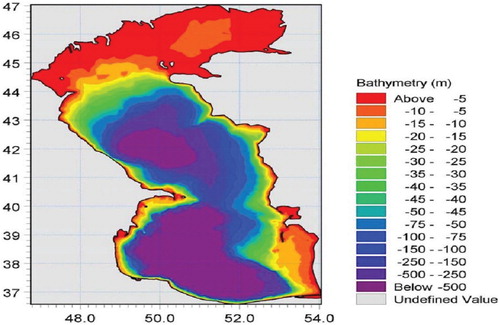
This study explores the impacts of climate change on wind power resources in the Caspian Sea. As a landlocked sea, the Caspian Sea is surrounded by five countries: Iran, Russia, Kazakhstan, Turkmenistan and Azerbaijan. The study area is located between latitude 36.5°N and 47°N, longitude 47°E and 54°E (Figure 1), and is bounded by Russia and Kazakhstan to the north, Iran to the south, Azerbaijan to the west and Turkmenistan to the east. The bathymetry of the area varies widely, from very shallow water with less than 5 m depth in the northern part to deep water exceeding 500 m in the middle and southern parts (Figure 1). With a water volume of about 78,200 km³ and an area of 371,000 km², the Caspian Sea is the largest inland water body in the world (Likens et al., 2009). Winds are the most typical hydrometeorological feature of the Caspian Sea. They mainly blow from the north and east. During the winter, easterly winds created as a result of the Asiatic anticyclone are dominant, while in the summer, northerly winds caused by the Azores high-pressure system blow frequently (Rusu & Onea, 2013). For such a massive water body, there is a limited number of weather stations to record wind speed and direction. Therefore, reanalysis data such as ERA-Interim obtained from the European Centre for Medium-Range Weather Forecasts (ECMWF) are considered as common wind data resources when long-term data are required. Details of the applied data are presented in the following subsection.

Figure 1. Depth variation in the study area, Caspian Sea (Allahdadi et al., 2004).

2.2. Data resources

The data sets used in this study for climate studies are obtained from CORDEX outputs, which are regional downscaling of GCMs. These outputs are derived by imposing boundary conditions from GCMs and running the model for a particular domain. Dealing with CORDEX, a domain is referred to as a region for which the regional downscaling takes place. In this regard, these models have been developed for different regions (14 regions or domains), together covering the whole globe. The CORDEX outputs for each domain, RCMs, usually provide climatic data with higher spatial and temporal resolution than the GCMs. The Caspian Sea domain is covered by the RCM of west Asia (WAS) with a spatial resolution of 0.44° in both latitude and longitude. Therefore, daily wind outputs of the RCM (WAS44i) have been obtained from the website for the study area. The wind components, including zonal and meridional wind at 10 m from the surface, are obtained. Before investigating climate change impacts, it is necessary to evaluate the consistency and accuracy of CORDEX outputs based on a reference data set. Owing to limited field observations and weather stations for such a large water body, the ERA-Interim reanalysis wind data with a 6 h interval are considered as reference data to assess CORDEX data for the historical period. Although many GCMs can be used to derive RCMs, in the case of our study area and for domain WAS, only the CORDEX outputs obtained from GCM named MPI-ESM-LR (Max Planck Institute for Meteorology low-resolution Earth System Model) are available. Figure 2 illustrates the mean annual wind speed for the 20 year period 1981–2000 for ERA-Interim and the RCM.

Figure 2. Mean annual wind speed for the historical period: (a) European Centre for Medium-Range Weather Forecasts (ECMWF) and (b) Max Planck Institute (MPI) wind simulations.

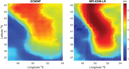
From Figure 2, it can be found that the RCM, meaning the MPI-ESM-LR, wind speed simulations overestimate wind speed over the sea area, while on the land surrounding the sea, the RCM slightly underestimates the wind speed. However, both data resources provide a similar trend, and there is a suitable consistency between the two data-set simulations. In general, a higher gradient in wind data can be found for the RCM simulations than the corresponding values for the reference data (ECMWF). The average wind speeds over 20 years for the reference and the RCM simulations over the whole area illustrated in Figure 2 are 3.92 and 3.85 m/s, respectively. Therefore, a good degree of similarity between the reference and the RCM wind climate can be found for the historical period.

Subsequent to verifying the RCM wind data, the outputs are used for climate change impact studies. In this regard, historical and future wind outputs of the CORDEX derived from MPI GCM for a 20 year period are used to compute wind power density in the past (1981–2000) and future (2081–2100). To project the future distribution of wind power in the study area, two scenarios standing for two representative concentration pathways (RCPs) of RCP4.5 and RCP8.5 are taken into consideration. RCPs are greenhouse gas concentration trajectories adopted by the Intergovernmental Panel on Climate Change in its fifth assessment report. In this regard, four RCPs, i.e. RCP2.6, RCP4.5, RCP6 and RCP8.5, have been selected, indicating radiative forcing values in W/m² in the year 2100. These RCPs are developed according to a wide range of possible changes in future anthropogenic greenhouse gas emissions. RCP2.6 is known as an optimistic scenario, RCP4.5 and RCP6 as medium scenarios, and RCP8.5 as the pessimistic scenario. This study employs CORDEX wind outputs for two RCPs of 4.5 and 8.5, which are commonly applied for climate change studies. More details about the future climate scenarios of the fifth assessment report can be found in Meinshausen et al. (2011).

2.3. Wind power computations

In general, long-term wind data are required for climate change impact studies, in which they are usually available for near-surface wind at 10 m. However, wind power is mainly computed at turbine hub-height, typically at 80–120 m. In this regard, near-surface wind data should be converted to turbine hub-height wind speed through an extrapolation technique. The extrapolation process is not an easy task because it is strongly dependent on the local conditions, such as roughness length (Stull, 2012). Thus, the power law is a commonly used expression that enables one to convert near-surface wind speed to any desired height following a limited number of local conditions (Equation 1): (1) $W_z=\frac{u_{\ast }}{k}\text{ln}\frac{z}{z_0}$(1) where $W_z$ is the wind speed at turbine hub-height (z), $u_{\ast }$ is the shear velocity, $k$ is the Von Karman constant, usually considered as 0.4, and $z_0$ is the roughness length. The sheer velocity is a function of the surface wind stress and the air density, and accurate calculation of these two parameters is a complex procedure owing to their dependency on other atmospheric variables such as pressure and temperature. Therefore, finding a suitable equation relating near-surface wind speeds to those of the turbine hub-height but depending on fewer variables is of great interest. In this regard, the following equation, based on only the roughness length ($z_0$), reference height ($z_{\text{ref}}$) and turbine height (z), is an appropriate alternative to determine the wind speed profile. (2) $\frac{W_z}{W_{\text{ref}}}=\frac{\text{ln}\left(\frac{z}{z_0}\right)}{\text{ln}\left(\frac{z_{\text{ref}}}{z_0}\right)}$(2) All of the variables in Equation (2) can be easily determined, except the roughness length, which is more complex. The surface roughness $z_0$ (in m) in onshore locations is constant, while in offshore areas it is mainly dependent on wind waves. For the offshore regions, the surface roughness can be computed as: (3) $\frac{z_0}{H_s}=1200{\left(\frac{H_s}{L_p}\right)}^{4.5}$(3) where $H_s$ and $L_p$ are the significant wave height and the wavelength of the peak wave (m), respectively.

The roughness length for the calm state was measured as about 0.2 mm, and the average roughness for a blown sea was estimated at about 0.5 mm, as stated by Manwell, McGowan, and Rogers (2010). Moreover, according to other studies (Powell, Vickery, & Reinhold, 2003; Yu, Chowdhury, & Masters, 2008), it can be found that the roughness length for high winds and hurricanes can vary between 2 and 20 mm. However, for our case (Caspian Sea), there are no reports indicating such high winds or hurricanes. Consequently, the wind state for the study area is considered a calm state. Furthermore, a study in the Caspian Sea revealed that the average roughness length is about 0.2 mm and calm state conditions are dominant in the area (Amirinia et al., 2017). Finally, taking wind speed at the turbine hub-height, the wind power density ($P_{\text{wind}}$) in terms of power (P) per unit area (A) or wind speed and air density can be computed as: (4) $P_{\text{wind}}=\frac{P}{A}=\frac{1}{2}{\rho }_{\text{air}}{W}^3$(4) where ${\rho }_{\text{air}}$ is the air density, which hereafter equals 1.225 kg/m³.

The main purpose of this study is to investigate the impacts of climate change on wind power in the Caspian Sea; therefore, detailed descriptions on roughness length, wind speed profile at turbine hub-height and extrapolation of wind speed to the desired level are beyond the scope of the manuscript. However, they can be found in the mentioned references (i.e. Powell et al., 2003; Yu et al., 2008; Amirinia et al., 2017).

2.4. ANFIS approach for post-processing

Data post-processing techniques are commonly used to modify or regionalize the outputs of numerical models to match more closely with those of the reference or real data. In this regard, regression-based models were traditionally used to bring the statistics of the computed data in line with the local measurements. However, these types of techniques often suffer from a lack of efficiency to catch nonlinear processes embedded in the phenomena. In the past decade, an ANFIS, with the advantages of both the artificial neural network and fuzzy systems, has attracted the attention of many researchers for time-series forecasting and analysis. However, fewer efforts have been devoted to employing this approach for data post-processing purposes. As observed from Figure 2, the climate data obtained from CORDEX simulations show a remarkable overestimation compared to the reference data, i.e. ERA-Interim. Therefore, even though this overestimation happens for both historical and future outputs of the climate model, for real evaluation and practical applications, a post-processing technique can help to provide more accurate estimations of the wind power in the area. Since the climate models are using complicated numerical approaches and they have passed many different validations, normality and other statistical tests, the historical and future outputs have been primarily investigated without any disturbance. Therefore, these data were first used to explore climate change impacts on wind power potential and their temporal distributions. Then, once the climate change impacts had been revealed, an ANFIS-based post-processing approach was taken into consideration to bring the results into the reference data range. This is an important step toward sustainable development and future plans to extract wind energy resources.

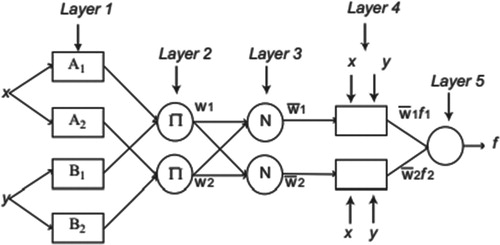
In brief, an ANFIS model combines transformed data through a membership function with if–then fuzzy rules and an inference system to derive the desired results. As it gains advantages from the features of both neural networks and fuzzy logic, the ANFIS model uses the learning ability of neural networks to define the input–output relationship and construct the fuzzy rules by determining the input structure (Alizdeh, Joneyd, Motahhari, Ejlali, & Kiani, 2015). It is noted that this study does not delve into detailed descriptions of the ANFIS model, and only the technique is applied from the MATLAB^® library; further explanations including mathematical expressions of the method can be found in the relevant references (Alizadeh, Rajaee, & Motahari, 2016; Aqil, Kita, Yano, & Nishiyama, 2007). However, to illustrate the scheme briefly, an ANFIS is usually assumed to consist of five layers, following one another. Figure 3 illustrates the schematic layout of a typical ANFIS consisting of five layers with two input variables of x and y. The first layer processes the input variables through a membership function. The input nodes in the first layer (represented in Figure 3 as A₁, A₂, B₁ and B₂) are linked to the nodes in the second layer multiplying with the incoming nodes. In the third layer, the normalized firing strength is calculated for each node (called weights w_i). The contribution of rules toward the output of the models is evaluated in this step. Finally, the last layer consisting of a single node gives the outputs of the ANFIS model. In this study, first the ANFIS model was trained using historical wind power data of CORDEX and ECMWF as the model input and output, respectively. Subsequently, the model was fed by future data computed from CORDEX–MPI simulations to predict the modified wind power for future scenarios. Dealing with the ANFIS model, four Gaussian membership functions were used for data processing in the first layer.

Figure 3. Schematic layout of the adaptive neuro-fuzzy inference system (ANFIS) model (Aqil et al., 2007). ERA = European Centre for Medium-Range Weather Forecasts ReAnalysis; MPI-ESM-LR = Max Planck Institute low-resolution Earth System Model; CORDEX = Coordinated Regional Climate Downscaling Experiment; RCP = representative concentration pathway.

2.5. Modeling procedures

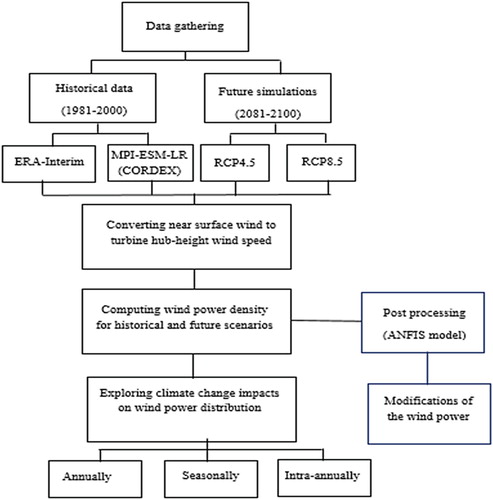
To establish the projection of wind power and its variability under future climate change scenarios, historical and future simulations of near-surface wind were obtained from CORDEX. Before computing the wind power from the wind speed, the historical climate data on wind speed were evaluated against reference data; here, ERA-Interim data (ECMWF) were used. Subsequent to the agreement between the two wind resources, CORDEX simulations of wind data for historical (1981–2000) and future outputs for two climatic scenarios of RCP4.5 and RCP8.5 were taken into consideration to determine climate change impacts. The CORDEX outputs were obtained for the GCM of MPI-EXM-LR, developed by the Max Planck Institute. Then, these data at 10 m were converted to the desired height, named turbine hub-height, through an extrapolation process. The converted wind speeds were used to compute wind power density. By comparing the wind power for historical and future periods, the climate change impact was revealed. The results of climate change impacts in terms of annual, seasonal and intra-annual variability were analyzed and mapped for the whole study area. Finally, a post-processing technique exploiting the ability of the ANFIS model was constructed and used to modify the wind power computed from CORDEX wind simulations, as CORDEX overestimates the wind speed compared to ECMWF wind data. In this regard, the mean annual values of wind power for the historical period of ECMWF and CORDEX were reorganized in a single-column matrix of input and outputs to train the ANFIS model. Furthermore, the ANFIS model was used to estimate the mean annual wind power in different nodes of the study area for future scenarios in the testing stage. The main steps of the study are summarized in Figure 4.

Figure 4. Schematic layout of the study.

3. Results and discussion

3.1. Annual variability of wind power

To evaluate the wind power distribution spatially, and to illustrate the impacts of climate change on future wind power resources, the mean annual wind power distributed over the whole study area was taken into consideration. To project the future climate of wind power, CORDEX near-surface wind simulations for historical (1981–2000) and two future scenarios of RCP4.5 and RCP8.5 are used for wind power computations at the turbine hub-height.

Figure 5 illustrates the mean annual wind power over the study area for historical and future periods. From Figure 5, it can be observed that the wind power over the study area has a quite varied distribution where for the middle part of the sea, the wind power is very high, exceeding 600 W per unit area, while for the southern part, the power decreases rapidly. Moreover, the gradient of wind power from offshore toward onshore or the surrounding land is strong. For example, offshore, the wind power in the middle latitude and for the middle part of the sea is higher than 600 W/m², while it decreases to as low as 100 W/m² in the eastern regions and the values are even less in western lands neighboring the sea. In general, moving from the northern part of the sea toward the middle latitude, wind power increases; and from the middle to lower latitude or southern part, the power decreases rapidly.

Figure 5. Projection of mean annual wind power over the study area for historical and future periods. RCP = representative concentration pathway.

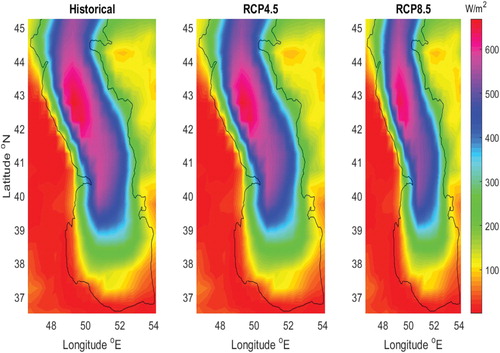
Considering climate change impacts on wind power distribution under the future scenarios, it can be seen that the historical projection of wind power has slightly higher values than the corresponding values for the future periods. Similarly, the power values for RCP4.5 are slightly stronger than those obtained for RCP8.5. However, the future changes in wind power compared to the historical projection reveal that climate change does not affect future wind power significantly. This is an important point for the future design and development of wind turbines in the study area. To illustrate mean annual future variations due to climate change impacts, relative changes in mean annual wind power for each scenario against historical projections have been computed, and the results are shown in Figure 6.

Figure 6. Relative changes in mean annual wind power for two representative concentration pathways: (a) RCP4.5; (b) RCP8.5.

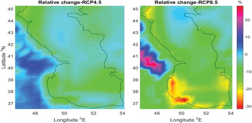
As observed from Figure 6, the future changes in wind power are not remarkable for most of the study area. Considering relative changes for RCP4.5, it can be derived that the future variation over the sea rarely exceeds 10%. Moreover, the negative signs indicated by the color map depict decreases in future wind power compared to historical values. Similarly, for RCP8.5, a decrease over the whole sea is expected to happen, in which the relative changes for RCP8.5 are slightly higher than for RCP4.5. The change for RCP8.5 reaches 20–30% in the south-east of the sea. Therefore, the climate change impacts on the mean annual wind power for both scenarios provide a low decrease over the sea, while the decrease is stronger in the southern part of the region where the wind power has lower values than in the other regions. Therefore, the regions in the middle parts of the sea have a higher potential for power extraction. Despite the slightly decreasing trend in wind power projection over the sea, for other surrounding land regions, especially in the eastern parts, a small increase in wind power is projected. This increase is intensified for RCP8.5. However, further analyses are required to enable the reliable development and installation of wind turbines, especially considering the temporal distribution of wind power and its future variation. The following subsections provide temporal projections of wind power in seasonal and monthly time scales for historical and future scenarios.

3.2. Seasonal variability of wind power

Owing to different temporal distribution over the seasons and also to variable demand on wind energy as a result of different seasonal climate and differences in industrial and human activity, seasonal assessment of the power distribution can provide suitable information for sustainable development. In this regard, wind power and its future variations for each season are computed separately, and the results are illustrated in Figures 7–10. Mean wind power values for December, January and February are integrated to compute the mean wind power for winter; similarly, spring covers March, April and May; summer includes June, July and August; and, finally, September, October and November are considered as autumn.

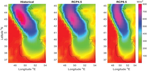
From Figure 7, the historical wind power has a slightly higher value than the corresponding values obtained from future scenarios. The pink color in the left panel illustrating the historical mean wind power for winter is more highlighted, meaning that it is stronger than the future ones. Considering two scenarios, RCP4.5 has a higher average than RCP8.5, whereas for the offshore locations in the middle and northern parts, the wind power distribution is higher for RCP8.5. The higher gradient of wind power for RCP8.5 than for the alternative scenario, RCP4.5, balances these higher values in the middle and northern parts with those of the lower ones in the eastern neighborhood of the sea. Comparing the distribution of winter with mean annual wind power (Figure 5), it can be derived that the trend in the winter is slightly different from that illustrated in the annual plots. In the seasonal illustration for winter, the trend of peak values extends from the high middle latitude toward the northern parts, while for the annual wind power, the trend is for peak values extending from the northern to the middle latitudes. In general, the average wind power in winter changes from 150 W/m² to 800 W/m² in the northern and middle parts of the sea. As the middle and northern parts have a relatively cold climate in winter and subsequently require more energy supply, wind power can be considered as a suitable option for energy supply as its distribution and power are remarkable for these areas. Moreover, future warming conditions do not change or decrease the wind power for these areas significantly.

Figure 7. Wind power distribution in winter for historical and future simulations. RCP = representative concentration pathway.

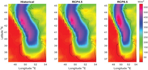
Wind power distributions for the spring season are presented in Figure 8. Regarding Figure 8, the wind power in spring has a similar spatial trend to the annual projections, while a different pattern for climate change impact projections can be found. However, the mean values of wind power in spring are lower than the mean annual values, and are also lower than in winter. The mean power in spring is in the range of 50–550 W/m², indicating lower wind power in spring and a calm state over the sea. Considering future projections of wind power, the color indicating the peak values of power is more intense for RCP8.5 than for RCP4.5, and also more intense than the corresponding historical values. Therefore, the locations with the highest potential for wind power, mainly in the middle latitudes, will experience an increase, whereas power is not expected to increase in the other regions.

Figure 8. Wind power distribution in spring for historical and future simulations. RCP = representative concentration pathway.

In a similar way, the results of wind power computations for historical and future projections in summer and autumn are illustrated in Figures 9 and 10, respectively.

Figure 9. Wind power distribution in summer for historical and future simulations. RCP = representative concentration pathway.

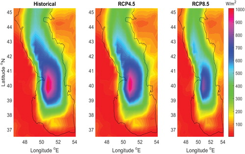
Figure 10. Wind power distribution in autumn for historical and future simulations. RCP = representative concentration pathway.

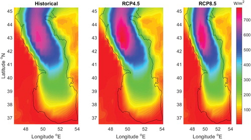
Figure 9 demonstrates that summer will experience relatively a strong decrease in wind power as a result of future climatic conditions. Moreover, there is an inverse spatial trend in the middle to northern latitudes compared with the annual, winter and spring seasons. In other words, for summer, the strongest winds blow in the low middle latitudes, whereas the general trends were found for the high middle and northern parts. This is promising as the middle and lower latitudes have warmer summers and higher demand for energy supply than the high middle and northern latitudes. Considering the climate change impacts, these future simulations of wind power provide lower values than the historical computations. Moreover, RCP8.5 shows that the future decrease in summer is more intense for RCP8.5 than for RCP4.5. Generally speaking, it is demonstrated that wind power in summer may exceed 1000 W/m², which is much higher than for the other seasons, as depicted earlier.

As illustrated in Figure 10, climate change does not notably affect the wind power distribution over the study area. However, for the middle parts of the sea, representing the highest potential of the power, a slight increase can be projected under future climatic conditions. Comparison of the spatial distribution of the power for autumn with those of the other seasons and annual projections shows that the spatial distribution has a roughly similar trend to the annual one. Moreover, the computed values of wind power in autumn are closer to the mean annual power than those computed for the other seasons.

To provide more details of the wind power variation for different seasons and different scenarios, mean values of wind power averaged over the whole study area are presented in Table 1. The results of seasonal analysis given in Table 1 show that the historical projections have higher power potential than the future simulations. However, the difference is negligible or not valuable. In general, the climate change impacts on seasonal distribution are different from one season to another. Moreover, the pattern is not monotonic; for winter and summer, the future simulations decrease remarkably in comparison with the historical values, with a higher rate of decrease for RCP8.5 than for RCP4.5, while for spring and autumn, the mean values of wind power do not differ significantly under the climate change scenarios. In addition, the seasonal projection for wind power revealed a high level of temporal distribution, with winter and summer being the seasons with the highest power, and spring being classified as the season with the lowest wind power potential.

Table 1. Mean seasonal wind power averaged over the whole study area.

Season	Historical	RCP4.5	RCP8.5
Winter	220	205	203
Spring	160	155	160
Summer	207	191.5	167
Autumn	182	186	183

Note: RCP = representative concentration pathway.

3.3. Intra-annual distribution of wind power

Intra-annual variability analysis is a common procedure by which to detect temporal distributions in climate change studies. It can provide details of the variation in power under future scenarios. Therefore, in this study, the mean value of wind power for historical and future scenarios was averaged over the whole study area and the results are illustrated in Figure 11. In Figure 11, the vertical axis represents mean wind power (in watts per unit area) and the horizontal axis represents month number (starting from January, denoted as month number 1, and continuing to December, denoted with the number 12). Therefore, the months with numbers 12, 1 and 2 represent the winter season; numbers 3, 4 and 5 are spring; numbers 6, 7 and 8 are summer; and numbers 9, 10 and 11 are used for autumn calculations.

Figure 11. Intra-annual variability of wind power under future climatic scenarios. RCP = representative concentration pathway.

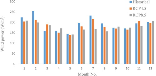
The monthly analysis of wind power depicted in Figure 11 presents a high level of intra-annual variability, with the winter and summer months having the highest rate of changes due to climate change impacts. Overall, January and July are the months with the highest decrease under climate change impacts. On the other hand, May, September and October are less influenced by future climatic conditions. February, January and July are the months with the highest potential for wind power and, conversely, March and May have the lowest wind power potential. In general, the future simulations of wind power illustrate lower values than the historical projections, and the simulations obtained from RCP8.5 have lower values than RCP4.5. However, the decrease is not consistent for all months and sporadic increases are observed for some months. Therefore, climate change is expected to impose a slightly decreasing trend on future wind power resources, although this trend may not be regular for all months and some inconsistencies may be found.

3.4. ANFIS post-processing approach for data modification of CORDEX

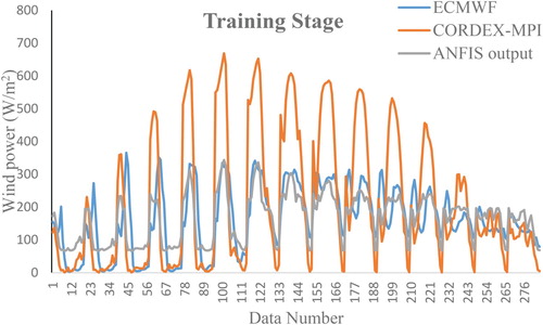
To be able to use the CORDEX estimations of wind power in real-world applications, consistent in magnitude with the reference data, the ANFIS model was developed, which used the CORDEX outputs as the predictor and the reference data as the predictand. This process was carried out to train the model and also to predict and modify the future simulations of the CORDEX outputs applied for wind power computations. The predictor and predictand mean annual wind power over the whole study area were converted or reshaped into a single-column matrix to meet the ANFIS model input requirements. After training and testing the model, the model outputs were reorganized to their normal form to represent the spatial power distribution. The overall performance of the model during the training process in terms of the coefficient of determination was calculated as R² = 0.59.

Figure 12 illustrates the CORDEX, ECMWF and ANFIS outputs for the training stage (for the historical period). As observed from Figure 12, the climate model in the study area reveals that the CORDEX simulations provide higher values of wind power in regions with a high energy potential. On the other hand, for the regions with lower potential for wind energy, the CORDEX simulations provide lower values than the corresponding wind power of ECMWF. Therefore, post-processing can be deemed as an appropriate option to modify these values toward the real values. The ANFIS outputs illustrated in Figure 12 indicate that the model in the training stage can be suitably used to bring the data into the reference data range. There is a good degree of similarity between the ANFIS outputs and those of the ECMWF-based data.

Figure 12. Results of the adaptive neuro-fuzzy inference system (ANFIS) model for the historical period. ECMWF = European Centre for Medium-Range Weather Forecasts; CORDEX = Coordinated Regional Climate Downscaling Experiment; MPI = Max Planck Institute.

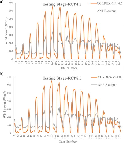
Subsequent to the model training, the tuned variables or weights were used to estimate wind power for the future scenarios. In this regard, two models were constructed separately to estimate wind power for RCP4.5 and RCP8.5. Figure 13 presents the results of the ANFIS models for the two future scenarios. According to Figure 13, the ANFIS model outputs for the future scenarios are remarkably lower than those obtained directly from the CORDEX model. In contrast, the model estimations for the places with lower potential are higher than those of the CORDEX-based simulations. Therefore, the ANFIS model attenuates the magnitude of the high-potential spots and also augments the magnitude of the locations with lower potential. However, the outputs of the ANFIS- and CORDEX-based computations have a homogeneous or similar trend, but differ in their magnitude. The results of the testing period are in line with those of the training period, in which the higher and lower estimations of CORDEX-based wind power were, respectively, decreased and increased in magnitude as the model outputs.

Figure 13. Results of the adaptive neuro-fuzzy inference system (ANFIS) model for two representative concentration pathways: (a) RCP4.5; (b) RCP8.5. CORDEX = Coordinated Regional Climate Downscaling Experiment; MPI = Max Planck Institute.

4. Conclusions

Global warming and climate change are ongoing issues whose impacts on different environmental, atmospheric and aquatic ecosystems are increasingly being considered. Renewable energy, as a good remedy by which to attenuate the effects and emissions of greenhouse gases, has attracted the attention of many researchers. The main purpose of this study was to investigate the impacts of climate change on wind power resources in the Caspian Sea. To do this, historical and future simulations (for a 20 year period) of near-surface wind speed were obtained from MPI-ESM-LR CORDEX outputs. The near-surface wind speed was converted to a turbine hub-height of 120 m and the transformed wind speed was used to compute wind power over the study area. The power distribution in terms of spatial and temporal variability for historical and two future climatic scenarios of RCP4.5 and RCP8.5 was taken into consideration. Moreover, an ANFIS-based model was developed to align the statistics of the wind power obtained from CORDEX data with those of reference data.

The results of wind power projections revealed that the study area has a suitable potential for energy extraction as the mean annual wind power reached over 800 W per unit area. The spatial distribution of wind power over the study area was quite variable, with the middle and northern parts of the sea having far higher potential for wind power than the southern part. In general, the future projections of wind power over the study area show a decreasing trend compared to the historical computations. However, the decrease has strong temporal and spatial distributions, in which the power may increase in particular regions of the sea. Considering the two investigated scenarios, it was found that RCP8.5 provided a higher gradient and rate of change than RCP4.5. This was supported by the results of relative change in wind power for future simulations against historical values, where the relative change for RCP4.5 was obtained in a range between 0 and −10%. However, corresponding values for RCP8.5 reached −20 to −30%, especially in the south-eastern part of the sea.

Considering temporal variability of wind power under future climatic conditions, it can be derived that the future wind power in winter and summer will decrease remarkably, while for spring and autumn the future changes are negligible. Moreover, it was found that winter and summer are the seasons with the highest wind power, while spring has the lowest power. The results of intra-annual variability demonstrated that February and July are the months with the highest rate of change, meaning a decrease in future scenarios. Simultaneously, they are considered, along with January, as the most months with the highest wind power potential. On the other hand, the spring and autumn months are expected to be affected least by future climatic conditions. Among the different months, May and October have the lowest rate of variation when future values are compared to historical values. Low values of wind power in spring may reflect the calm state over the sea.

The results of this study are promising in view of developing and installing wind turbines in the study area for energy extraction due to the suitable potential of wind power, especially in the middle and northern parts. Moreover, it was found that future climatic conditions will not change the wind power distribution in the area significantly. The seasonal wind power resources show higher potential for winter and summer, when there is increased energy demand for the area. Therefore, there is good consistency between the demand for and supply of energy. Finally, it should be added that the real potential of the area is lower than that computed from CORDEX simulations, even though the modified values are still remarkable and imply the suitability of the area for wind power extraction. The findings of this study should prove beneficial for energy policymakers and strategists to plan for developments in the wind power sector, considering the variability of wind power under future climatic scenarios. Future research could focus on uncertainties associated with the RCMs and the efficiency of different climate models for the area.

Acknowledgments

We acknowledge the financial support of this research by the Hungarian State and the European Union under the EFOP-3.6.1-16-2016-00010 project.

Disclosure statement

No potential conflict of interest was reported by the authors.

Appendix.

Table A1. List of abbreviations.

Abbreviation	Definition
ANFIS	Adaptive neuro-fuzzy inference system
CORDEX	Coordinated Regional Climate Downscaling Experiment
ECMWF	European Centre for Medium-Range Weather Forecasts
GCM	Global circulation model
MPI	Max Planck Institute
RCM	Regional climate model
RCP	Representative concentration pathway

References

- Alizadeh, M. J., Rajaee, T., & Motahari, M. (2016). Flow forecasting models using hydrologic and hydrometric data. Proceedings of the Institution of Civil Engineers-Water Management.
- Alizdeh, M. J., Joneyd, P. M., Motahhari, M., Ejlali, F., & Kiani, H. (2015). A wavelet-ANFIS model to estimate sedimentation in dam reservoir. International Journal of Computer Applications, 114(9), 19–25. doi: 10.5120/20007-1958
- Allahdadi, M. N., Chegini, V., Fotouhi, N., Golshani, A., Jandaghi, A. M., Moradi, M., … Taebi, S. (2004). Wave modeling and Hindcast of the Caspian Sea. Proceedings of the 6th International Conference on Coasts, Ports, and Marine Structures, Tehran, Iran.
- Amirinia, G., Kamranzad, B., & Mafi, S. (2017). Wind and wave energy potential in southern Caspian Sea using uncertainty analysis. Energy, 120, 332–345. doi: 10.1016/j.energy.2016.11.088
- Aqil, M., Kita, I., Yano, A., & Nishiyama, S. (2007). Analysis and prediction of flow from local source in a river basin using a Neuro-fuzzy modeling tool. Journal of Environmental Management, 85(1), 215–223. doi: 10.1016/j.jenvman.2006.09.009
- Beyaztas, U., Salih, S. Q., Chau, K.-W., Al-Ansari, N., & Yaseen, Z. M. (2019). Construction of functional data analysis modeling strategy for global solar radiation prediction: Application of cross-station paradigm. Engineering Applications of Computational Fluid Mechanics, 13(1), 1165–1181. doi: 10.1080/19942060.2019.1676314
- Chang, T.-J., Chen, C.-L., Tu, Y.-L., Yeh, H.-T., & Wu, Y.-T. (2015). Evaluation of the climate change impact on wind resources in Taiwan Strait. Energy Conversion and Management, 95, 435–445. doi: 10.1016/j.enconman.2015.02.033
- Cheng, C.-T., Lin, J.-Y., Sun, Y.-G., & Chau, K. (2005). Long-term prediction of discharges in Manwan Hydropower using adaptive-network-based fuzzy inference systems models. International Conference on Natural Computation.
- Davy, R., Gnatiuk, N., Pettersson, L., & Bobylev, L. (2018). Climate change impacts on wind energy potential in the European domain with a focus on the Black Sea. Renewable and Sustainable Energy Reviews, 81, 1652–1659. doi: 10.1016/j.rser.2017.05.253
- de Jong, P., Barreto, T. B., Tanajura, C. A., Kouloukoui, D., Oliveira-Esquerre, K. P., Kiperstok, A., & Torres, E. A. (2019). Estimating the impact of climate change on wind and solar energy in Brazil using a South American regional climate model. Renewable Energy, 141, 390–401. doi: 10.1016/j.renene.2019.03.086
- Dosio, A. (2016). Projections of climate change indices of temperature and precipitation from an ensemble of bias-adjusted high-resolution EURO-CORDEX regional climate models. Journal of Geophysical Research: Atmospheres, 121(10), 5488–5511.
- Fotovatikhah, F., Herrera, M., Shamshirband, S., Chau, K.-W., Faizollahzadeh Ardabili, S., & Piran, M. J. (2018). Survey of computational intelligence as basis to big flood management: Challenges, research directions and future work. Engineering Applications of Computational Fluid Mechanics, 12(1), 411–437. doi: 10.1080/19942060.2018.1448896
- Khanali, M., Ahmadzadegan, S., Omid, M., Nasab, F. K., & Chau, K. W. (2018). Optimizing layout of wind farm turbines using genetic algorithms in Tehran province, Iran. International Journal of Energy and Environmental Engineering, 9(4), 399–411. doi: 10.1007/s40095-018-0280-x
- Koenigk, T., Berg, P., & Döscher, R. (2015). Arctic climate change in an ensemble of regional CORDEX simulations. Polar Research, 34(1), 24603. doi: 10.3402/polar.v34.24603
- Likens, G., Benbow, M., Burton, T., Van Donk, E., Downing, J., & Gulati, R. (2009). Encyclopedia of inland waters.
- Manwell, J. F., McGowan, J. G., & Rogers, A. L. (2010). Wind energy explained: Theory, design and application. Seattle, USA: John Wiley & Sons.
- Mariotti, L., Diallo, I., Coppola, E., & Giorgi, F. (2014). Seasonal and intraseasonal changes of African monsoon climates in 21st century CORDEX projections. Climatic Change, 125(1), 53–65. doi: 10.1007/s10584-014-1097-0
- Meinshausen, M., Smith, S. J., Calvin, K., Daniel, J. S., Kainuma, M., Lamarque, J.-F., … Riahi, K. (2011). The RCP greenhouse gas concentrations and their extensions from 1765 to 2300. Climatic Change, 109(1–2), 213–241. doi: 10.1007/s10584-011-0156-z
- Moazenzadeh, R., Mohammadi, B., Shamshirband, S., & Chau, K.-w. (2018). Coupling a firefly algorithm with support vector regression to predict evaporation in northern Iran. Engineering Applications of Computational Fluid Mechanics, 12(1), 584–597. doi: 10.1080/19942060.2018.1482476
- Panapakidis, I. P., Michailides, C., & Angelides, D. C. (2019). A data-driven short-term forecasting model for offshore wind speed prediction based on computational intelligence. Electronics, 8(4), 420. doi: 10.3390/electronics8040420
- Petković, D., Ćojbašić, Ž, Nikolić, V., Shamshirband, S., Kiah, M. L. M., Anuar, N. B., & Wahab, A. W. A. (2014). Adaptive neuro-fuzzy maximal power extraction of wind turbine with continuously variable transmission. Energy, 64, 868–874. doi: 10.1016/j.energy.2013.10.094
- Porté-Agel, F., Wu, Y.-T., & Chen, C.-H. (2013). A numerical study of the effects of wind direction on turbine wakes and power losses in a large wind farm. Energies, 6(10), 5297–5313. doi: 10.3390/en6105297
- Powell, M. D., Vickery, P. J., & Reinhold, T. A. (2003). Reduced drag coefficient for high wind speeds in tropical cyclones. Nature, 422(6929), 279–283. doi: 10.1038/nature01481
- Pryor, S. C., & Barthelmie, R. (2010). Climate change impacts on wind energy: A review. Renewable and Sustainable Energy Reviews, 14(1), 430–437. doi: 10.1016/j.rser.2009.07.028
- Qasem, S. N., Samadianfard, S., Kheshtgar, S., Jarhan, S., Kisi, O., Shamshirband, S., & Chau, K.-W. (2019). Modeling monthly pan evaporation using wavelet support vector regression and wavelet artificial neural networks in arid and humid climates. Engineering Applications of Computational Fluid Mechanics, 13(1), 177–187. doi: 10.1080/19942060.2018.1564702
- Reyers, M., Pinto, J. G., & Moemken, J. (2015). Statistical–dynamical downscaling for wind energy potentials: Evaluation and applications to decadal hindcasts and climate change projections. International Journal of Climatology, 35(2), 229–244. doi: 10.1002/joc.3975
- Rusu, E., & Onea, F. (2013). Evaluation of the wind and wave energy along the Caspian Sea. Energy, 50, 1–14. doi: 10.1016/j.energy.2012.11.044
- Sailor, D., Hu, T., Li, X., & Rosen, J. (2000). A neural network approach to local downscaling of GCM output for assessing wind power implications of climate change. Renewable Energy, 19(3), 359–378. doi: 10.1016/S0960-1481(99)00056-7
- Salih, S. Q., Allawi, M. F., Yousif, A. A., Armanuos, A. M., Saggi, M. K., Ali, M., … Chau, K.-W. (2019). Viability of the advanced adaptive neuro-fuzzy inference system model on reservoir evaporation process simulation: Case study of Nasser Lake in Egypt. Engineering Applications of Computational Fluid Mechanics, 13(1), 878–891. doi: 10.1080/19942060.2019.1647879
- Shamshirband, S., Keivani, A., Mohammadi, K., Lee, M., Hamid, S. H. A., & Petkovic, D. (2016). Assessing the proficiency of adaptive neuro-fuzzy system to estimate wind power density: Case study of Aligoodarz, Iran. Renewable and Sustainable Energy Reviews, 59, 429–435. doi: 10.1016/j.rser.2015.12.269
- Shin, J.-Y., Jeong, C., & Heo, J.-H. (2018). A novel statistical method to temporally downscale wind speed Weibull distribution using scaling property. Energies, 11(3), 633. doi: 10.3390/en11030633
- Solaun, K., & Cerdá, E. (2020). Impacts of climate change on wind energy power – Four wind farms in Spain. Renewable Energy, 145, 1306–1316. doi: 10.1016/j.renene.2019.06.129
- Stull, R. B. (2012). An introduction to boundary layer meteorology. Oslo, Norway: Springer Science & Business Media.
- Tobin, I., Jerez, S., Vautard, R., Thais, F., Van Meijgaard, E., Prein, A., … Nikulin, G. (2016). Climate change impacts on the power generation potential of a European mid-century wind farms scenario. Environmental Research Letters, 11(3), 034013. doi: 10.1088/1748-9326/11/3/034013
- Viviescas, C., Lima, L., Diuana, F. A., Vasquez, E., Ludovique, C., Silva, G. N., … Lucena, A. F. (2019). Contribution of variable renewable energy to increase energy security in Latin America: Complementarity and climate change impacts on wind and solar resources. Renewable and Sustainable Energy Reviews, 113, 109232. doi: 10.1016/j.rser.2019.06.039
- Winstral, A., Jonas, T., & Helbig, N. (2017). Statistical downscaling of gridded wind speed data using local topography. Journal of Hydrometeorology, 18(2), 335–348. doi: 10.1175/JHM-D-16-0054.1
- Yang, H.-F., & Chen, Y.-P. P. (2019). Representation learning with extreme learning machines and empirical mode decomposition for wind speed forecasting methods. Artificial Intelligence, 277, 103176. doi: 10.1016/j.artint.2019.103176
- Yaseen, Z. M., Sulaiman, S. O., Deo, R. C., & Chau, K.-W. (2019). An enhanced extreme learning machine model for river flow forecasting: State-of-the-art, practical applications in water resource engineering area and future research direction. Journal of Hydrology, 569, 387–408. doi: 10.1016/j.jhydrol.2018.11.069
- Yu, B., Chowdhury, A. G., & Masters, F. J. (2008). Hurricane wind power spectra, cospectra, and integral length scales. Boundary-Layer Meteorology, 129(3), 411–430. doi: 10.1007/s10546-008-9316-8