Simulation of cargo VOC emissions from petroleum tankers in transit in Canadian waters

Abstract

The emissions of volatile organic compounds (VOCs) from petroleum product tankers potentially represent a significant source of VOCs in port cities. Emission factors are used to estimate the produced VOCs. VOC emissions from transit operations were simulated using a two part model of heat and mass transfer. Using local meteorological data of air temperatures, solar radiation and wind speed, the heat transfer within the tank was modeled. Results showed that bulk cargo temperature remained relatively steady at 25–28°C, the oil surface oscillated diurnally by 1–2°C, and the deck temperature oscillates diurnally by 15–20°C. The solar insolation had the largest effect on the tank temperatures. VOC emissions for two crude oils and gasoline, two tank configurations, and two meteorological conditions were estimated using a model derived from a mass balance on the tank and the obtained temperature profile. Only 3 of 8 scenarios had pressure increases large enough to cause venting of VOC. C2-C5 compounds constituted the majority of VOCs released from crude oils and ethanol made up the majority of the VOCs released from the gasoline carrying barge. The calculated daily emission factors for crude oil and gasoline (barge) were 10 mg/L/day and 135 mg/L/day respectively.

KEYWORDS:

• VOCs emission
• tanker transit
• numerical simulation
• temperature variation

1. Introduction

Volatile organic compounds (VOCs) are a wide group of organic compounds which evaporate at atmospheric conditions easily because of their high vapor pressure. VOC evaporation from oil not only wastes fuel, but is also a safety concern and creates local air pollution, causing to the formation of ground-level ozone. Oil tankers are responsible for the vast majority of oil movement worldwide, moving crude oil from the point of extraction to refineries (Chow, 2009). VOC emissions from tanker operations could potentially be a large source of local pollutants in and around petroleum terminals, and while in transit in the open ocean. To date, there has been little work concerning the VOC emissions from oil tankers during transit, which is the main purpose of this paper. A new method using a two-part model of heat and mass transfer within the tank was applied to simulate VOC emissions from transit operations. The estimated daily emission factors for MSB and gasoline (barge only) are significantly lower than the emission factors suggested by the EPA for crude oil and gasoline, but it would provide good reference for VOC emissions under the colder climate like Canada.

Production, storage and transport of crude oil and gasoline produce emissions of VOCs (DeLuchi, 1993). The main sources of VOC emissions at oil terminals are from storage tanks and tanker operations including loading/unloading and transit operations of the oil tankers (Tamaddoni, Sotudeh-Gharebagh, Nario, Hajihosseinzadeh, & Mostoufi, 2014). During loading, gases in the oil tank saturated with VOCs are displaced by incoming petroleum (US EPA, 2008). In the absence of equipment to capture the VOCs, as is the case with many petroleum ports, they are released into the air. After loading and during transit volatiles continue to evaporate from the surface of the petroleum cargo, increasing the pressure until venting is necessary to protect the integrity of the tank (US EPA, 2008). Tank venting is a regular occurrence during transport of petroleum products.

Crude oil is typically stored at refineries before being processed into petroleum products and as with transit of petroleum products in tankers, some of the volatile components of the oil evaporate or are displaced from storage tanks (DeLuchi, 1993). Emissions from storage tanks are more widely discussed in literature (Dakhel & Rahimi, 2004; Oldervik, Neeraas, Strom, Martens, & Meek-Hansen, 2000; Pasley & Clark, 2000; Paulauskienea, Zabukasb, & Vaitiek-unasc, 2009; Peress, 2001; Rota, Frattini, Astori, & Paludetto, 2001; Tamaddoni et al., 2014). Pasley and Clark (2000) developed a model for small- and full-scale tanks using AEA Technology's CFX4. A detailed computational fluid dynamics (CFD) study of the wind speeds and flow structures above and around the tanks was presented and validated by a series of 2-D measurements. The homogenization time of two layers of crude oil from different reservoirs in 19,000 m³ floating roof storage tanks was predicted (Dakhel & Rahimi, 2004).

Paulauskienea et al. (2009) studied VOC concentrations in oil terminal storage tank parks and evaluated the effect of oil product type, the level of an oil product in the storage tank, storage tank construction and the meteorological conditions. An experimental study was conducted to characterize VOCs emitted from storage tanks of crude oil in a large-scale oil export terminal (Tamaddoni et al., 2014). Experimental results showed that the crude oil absorption process can be adapted to the marine terminal for recovering emitted gases.

Although oil tankers are the main method for oil transportation from export terminals to refineries, there are limited studies available on VOC emissions from the transported crude oil (Martens, Oldervik, Neeraas, & Strøm, 2001; Rudd & Hill, 2001). Since the loading process produces the largest amount of VOCs, it is the most studied (Hassanvand, Hashemabadi, & Bayat, 2010; Karbasian, Kim, Yoon, Ahn, & Kim, 2017; Lee, Choi, & Chang, 2013; Milazzo, Ancione, & Lisi, 2017). Martens et al. (2001) developed a model to determine the evaporation rate and emissions from various crude oil types and cargo handling practices. They calculated the Non-Methane Volatile Organic Compound (NMVOC) emissions and proposed an absorption processes for VOC recovery as a lower cost, less energy intensive alternative to liquefaction. Milazzo et al. (2017) studied the scale of emissions of VOCs associated with ship-loading operations of petroleum products in refineries and then mapped the diffusion of such pollutants for a case-study by using a dispersion model and GIS software. Karbasian et al. (2017) examined different cases with a combination of a swirl unit and a U-bend through a numerical study with experimentation validation. A new approach was proposed to reduce the VOC formation notably during the loading process.

The simulation of VOC emissions from tanker during transit involves long computation time and large computation resource because the tanker often is very large and transportation will last long time. Transit emissions are highly sensitive to temperature of the cargo. In present work, computational heat transfer was utilized to calculate the heat transfer and determine the temperature distribution within the tank during a week of diurnal cycles utilizing metrological data from Montreal and Vancouver. The output of the temperature model was input into a mass transfer model of the evaporation of volatile species within the tank. Finally, transit emission factors were determined from the mass transfer model to evaluate the environment impact. The same method for simulating VOC emissions from tankers can’t be found from the literatures. The method can simulate VOC emissions from tankers during transportation several weeks with acceptable computation time.

The emissions from tanker operations (loading and transit) are currently estimated using emission factors first produced by the US EPA (AP-42 chapter 5.2) in 1972 and updated in 1995 (US EPA, 2008). In addition to their age, these emission factors do not represent the more volatile crude oils, including dilbit, and are in need of updating. This work presents transit emission factors from eight different scenarios examining two different climate conditions: Montreal and Vancouver; three different cargos: sweet light crude, dilbit and gasoline; and two different vessel configurations: a long-range crude oil tanker and a shallow draft barge.

2. Model description

Montreal and Vancouver were chosen as the representative metrological conditions since they are two of the larger crude oil-exporting ports in Canada and in major urban centers where local pollution is of concern. In order to simulate the heat transfer and VOC mass transfer within the tank during transit, a number of assumptions were used:

1. Natural convection within the oil and air gap is not considered and only conduction is considered. Due to solar heating of the deck and the cooling effect of the water on the hull bottom, the cargo and air density would decrease from bottom to top, inhibiting natural convection.

2. The tank headspace is nitrogen saturated with VOCs at the beginning of the mass transfer simulations. Tankers utilize inert gas in the head space for safety and it is assumed based on previous studies that the nitrogen has become saturated during the loading of the cargo (Rudd & Hill, 2001).

3. The tank has a release valve which opens at a pressure of 115 kPa. After release the tank pressure drops to 107 kPa and the valve closes.

4. Radiative heat transfer between the deck and the oil was not included in the heat transfer model due to the low temperature difference between the two (≤17°C).

5. Headspace in the tank, as well as the liquid phase, is assumed to be of homogeneous composition at a given time and interphase gradients in concentration are negligible.

2.1. Model geometry

Two types of vessels were used in the heat transfer model to determine the oil temperature profile: an intermediate, Panamax crude oil tanker and a shallow draft barge. The Laurentia Desgagnes was chosen as the representative crude oil tanker, as it represents a typical tanker found in Canadian waters. It is a medium-sized oil tanker with a capacity of 514,000 BBL (barrels of oil). It contains twelve symmetrical tanks, two of which are bow tanks of smaller capacity than the other ten as shown in Figure 1. The arrangement and dimensions of one of the ten interior tanks were used for this simulation.

Figure 1. Top view of Laurentia Desgagnes.

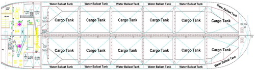
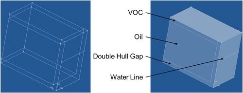
The tank measures approximately 24 m tall, 16 m wide and 28 m long and a full load draft, the distance between the waterline and hull bottom, of 9.5 m was assumed. Crude oil tankers have a double hull to prevent oil spills, in the Laurentia Desgagnes the air gap between hulls is approximately 1.4 m. With these dimensions, a three volume model was created in ANSYS, shown in Figure 2. The computation domain of a tank consisted of three volumes: the liquid cargo, the vapor headspace, and the air gap between the double hulls. The tank was considered to be 90% full, giving a headspace volume 10% of the total. Steel plates enclose the control volume and separated the oil from the air gap. In order to simplify the model, the separators are neglected, because the separators are thin with high thermal conductivity and the curvature on the outer bottom corner of the tank is neglected. The structured grid (Ghalandari, Shamshirband, Mosavi, & Chau, 2019) was meshed for computational domains to obtain the more accurate numerical result. About 40,000 hexahedron grids were used for computation.

Figure 2. ANSYS volume model of tank from Laurentia Desgagnes product tanker.

The model for the shallow draft barge tank is a similar design to the crude oil tank, but with dimensions of 6.0 m long, 5.3 m tall and 8.7 m wide, the thickness of air hull is 0.69 m and the draft is 3.95 m. Again the tank is assumed to be 90% full.

2.2. Crude oils

Two types of crude oil that represent light/medium crude oils typically produced and transported in Canada were simulated. The properties and light ends of these crude oil blends are shown in Table 1; the heavy non-volatile components are not listed. The Cold Lake Blend is a dilbit produced from Canadian oil sands operations and is mixed with a diluent for transport by pipeline. It contains high amounts of C4-C7 compounds from the diluent. The Mixed Sweet blend is a conventionally produced light crude oil blend produced in Western Canada and is often the reference crude oil blend used for pricing reports. It contains some dissolved ethane and propane. It is typically piped to the Superior terminal and further transported by pipeline, great lake tanker or rail car.

Table 1. Oil properties.

Properties	Cold Lake Blend (CLB)	Mixed Sweet Blend (MSB)	Gasoline
Density (m^3/kg)	842	822	775
Molecular Weight	173.3	213.1	114
Viscosity (Pa.s)	4.68 × 10^−3	4.04 × 10^−3	1.0 × 10^−3
Light Ends (vol%)
Ethane	0	0.0012	0
Propane	0	0.01351	0
Isobutane	0.0299*	0.03721	0.0315
n-Butane		0.08495	0
Isopentane	0.1575*	0.03885	0.1743
n-Pentane		0.05467	0.0356
n-Hexane	0.1062	0.03747	0.1450
n-Heptane	0.0565	0.02756	0.1368
n-Octane	0.0314	0.01956	0.0836
n-Nonane	0.0172	0.01501	0.0186
n-Decane	0.0075	0.00155	0.0995
Benzene	0.0049	0.00754	0.0037
Toluene	0.0069	0.02072	0.0702
Ethylbenzene	0.0008	0.00465	0.0207
Xylenes	0.0049	0.02378	0.0091
Ethanol	0	0	0.05

Note: *Represents mole fraction of all butanes and pentanes.

2.3. Heat transfer model

The general transient energy transfer equation for air, oil and VOCs was used to calculate the temperature distribution: (1) $\frac{\mathrm{\partial }}{\mathrm{\partial }t}\left(\rho h\right)+\mathrm{\nabla }.\left(\overrightarrow{v}\rho h\right)=\mathrm{\nabla }.\left(k\mathrm{\nabla }T\right)+S_h$(1) where ρ is density (kg/m³), h is sensible enthalpy (J/kg), $h={\int }_{T_{ref}}^T{c}_{p}dT$, k is conductivity (W/m.K), T is temperature (K), S_h is volumetric heat source (W/m³). The solar insolation, I (W/m²) was translated into a heat generation (W/m³) in the deck volume using the following: (2) $\overline{q}=\frac{A\times I}{t_s}$(2) where A is solar absorbance (0.8 for tankers with red deck), I is solar insolation (W/m²), t_s is thickness of steel (m). The heat transfer in the tank was simulated using ANSYS FLUENT software. The hourly solar insolation was input and the heat generation calculated using a UDF (User Defined Function) in ANSYS.

To simplify temperature used for mass transfer model in the MATLAB mass transfer model, a fitted function was used to model the changing temperature over a series of days. (3) $T=T_0+A\sin \left(\pi \frac{t-t_c}{\omega }\right)+bt$(3) where T₀, A, b, t_c and ω are fitted constants.

2.4. Mass transfer model

To describe mass transfer from the liquid phase to the gas phase, a mathematical model was built MATLAB, modeling each of the volatile components. It is assumed that diffusion within each phase is rapid relative to the mass transfer rate between phases. Based on the two-film theory and the gas-side mass transfer resistance being negligible compared to the liquid-side resistance, mass transfer to gas phase is derived from a simple mass balance on the tank, described by: (4) $\begin{array}{rl}\frac{d{C}_{g,i}}{dt}& =-\frac{V_L}{V_g}\frac{d{C}_{L,i}}{dt}\end{array}$(4) (5) $\begin{array}{rl}\frac{d{C}_{L,i}}{dt}& =k_{L}a(C^{\ast }-C_L)\end{array}$(5) (6) $\begin{array}{rl}{C}^{\ast }& =\frac{p_i}{v_p{\propto }_i}\left(\frac{M_i}{M_T}\right){\rho }_T\end{array}$(6) where C_g,i is the concentration of species i in the gas phase (kg/m³), C_L,i is the concentration of species i in the liquid phase (kg/m³), V_L is the volume of liquid in the tanker (m³), V_g is the volume of gas in the headspace of the tanker (m³), k_L is the liquid side mass transfer coefficient (m/s) for species i, a is the specific surface area (m²/m³), C* is the concentration of species i in the liquid phase that would be in equilibrium with the gas phase (kg/m³), p_i is the partial pressure of species i (kPa), v_p is the vapor pressure of species i (kPa), α_i is the activity coefficient of species i in the petroleum mixture, M_i is the molar mass of species i (g/mol), M_T is the molar mass of the mixture in the liquid phase (g/mol) and ρ_T is the total density of the liquid mixture (kg/m³). The liquid side mass transfer coefficient was estimated using the following expressions (Treybal, 1980): (7) $\begin{array}{rl}\frac{k_L\delta }{D_{AB}}& =Sh=3.41\end{array}$(7) (8) $\begin{array}{rl}{D}_{AB}& =\frac{117.3\times {10}^{-18}{M_T}^{0.5}T}{\mu {v_A}^{0.6}}\end{array}$(8) where D_AB is Diffusivity of species in bulk gas mixture (m²/s), T is temperature of bulk gas mixture (K), μ is solution viscosity (kg/m.s), υ_A is the solute molar volume at normal boiling point (m³/kmol), δ is characteristic length or film thickness (m) and Sh is the Sherwood number. The film thickness or characteristic length was estimated from the above equation using published volumetric mass transfer coefficients for benzene in oil (Hsieh, Babcock, & Stenstrom, 1993).

Properties of the volatiles species in the oil were taken from the steady state process simulation software VMGSim, utilizing Peng-Robinson equations of state to calculate vapor pressures and activity coefficients.

The release events were simulated for Montreal and Vancouver meteorological data, Cold Lake Blend, Mixed Sweet Crude and Gasoline, product tanker and barge. With the exception of the first scenario, the surface temperature profile was used in the mass transfer simulation. The first scenario utilized the VOC average temperature, an average of oil surface temperature, headspace middle temperature at X = 23 and the deck temperature.

2.5. Boundary conditions

For the heat transfer model July metrological conditions were as high temperatures and solar insolation during the peak of summer represents the maximum potential for tanker heating and VOC release. These conditions represent the hottest week in July over a 5 years period from 2013 to 2017. Wind speed and air temperature were obtained from Environment Canada historical climate data (Environment Canada, 2018). Solar insolation data from Environment Canada, but compiled by Weatherstats.ca was used for Montreal conditions, but for Vancouver a time-average Gaussian distribution based on July mean daily solar insolation was used as no hourly insolation data was available (Weatherstats.ca., 2018).

The deck is the main source of heat addition to the control volume through solar insolation and the external air temperature. The deck was defined using a mixed boundary condition of convection (wind and air external temperature) with heat generation (solar insolation). An external emissivity of 0.9 was used to calculate the radiation heat transfer between the deck and the surrounding external environment. As previously discussed this was transformed into a heat generation rate per volume using steel wall of 0.026 m thickness.

The wind speed data was used to determine a transient convection heat transfer coefficient on the deck and side of the tanker: (9) $H=11.6+7\times \sqrt{V_w}$(9) where V_w is wind speed (m/s) from the hourly meteorological data. The simulation was conducted on a single tank adjacent to three other tanks and assuming identical conditions in the surrounding tanks. Symmetry boundary conditions with zero heat flux were used for the three shared tank interior walls. The exterior wall of the tank represents a portion of the tanker’s hull with sections above and below the water line. The external hull is a double hull configuration with an air gap between the tank wall and the external wall. The underwater boundary condition applies to the side exterior wall and the bottom wall. As the heat transfer from the water to the steel external wall would be very high compared to that within the double hull air gap, the exterior wall temperature was set equal to the water temperature, 21.3°C and 10°C for the Montreal and Vancouver cases respectively. This temperature was held constant throughout the simulation. The exterior wall above the waterline was subjected to heat transfer due to convection from wind as Equation (7).

The historical average temperatures of 21.3°C and 18°C for the month of July for Montreal and Vancouver respectively were used as the initial cargo temperature.

2.6. Numerical procedures

The transient external temperature, convection heat transfer coefficient and insolation heat source were employed by UDF.

The transient temperature distribution of the tank being simulated during one week was computed first. The computation time step was set 3 s and data was saved every 1200 steps or one hour to be consistent with meteorology data collection time. The VOCs calculation was conducted after the temperature computation.

The rate of VOCs into the headspace was determined by solving a set of 32 ODEs that corresponded to the gas and liquid phases (Equations 4(5) $\begin{array}{rl}\frac{d{C}_{L,i}}{dt}& =k_{L}a(C^{\ast }-C_L)\end{array}$(5) and 5(6) $\begin{array}{rl}{C}^{\ast }& =\frac{p_i}{v_p{\propto }_i}\left(\frac{M_i}{M_T}\right){\rho }_T\end{array}$(6) , respectively) for each species listed in Table 1. To solve the set of equations, Matlab ode45 solver was utilized. At initial time, the VOCs headspace is filled with nitrogen saturated with VOCs and the pressure is considered to be atmospheric (101 kPa). The mass transfer model determines VOC evaporation due to increasing cargo temperature into the headspace until the pressure reaches 115 kPa. At this point, the mass transfer simulation is stopped and the mass of VOCs that would be released from the headspace during a pressure release from 115 to 107 kPa was calculated. The daily emission factor was calculated based on the mass of VOCs released. The new mass of VOCs in the headspace was calculated and the mass transfer simulation restarted with a new intercept for the temperature profile of the time the release occurred.

3. Results and discussions

3.1. Average temperature trends

The selected one-week meteorological conditions in Montreal and Vancouver are shown in Figure 3, which is referred to as the ‘extreme conditions' of metrological data based on 5 years from 2013 to 2017. Figure 3 shows the temperatures within the tank (solid lines) over the course of the week overlaid with the external temperature profile (dashed line), wind speed (dotted line) and solar insolation (filled area). The deck temperature fluctuates diurnally by 15–20°, which is much more than the temperatures of the VOC headspace and the oil temperature. During the day the deck temperature is 5–8° hotter than the external temperature indicating that the solar insolation has the greatest effect on the deck temperature and subsequently the oil temperature. Under these conditions, convection (wind) would transfer heat from the deck to the atmosphere, limiting deck temperature. Higher atmospheric temperatures would reduce this heat loss and allow the deck to reach higher temperatures, as seen near the end of the week in the Montreal simulation. It is for this reason that the maximum deck temperature generally follows the atmospheric temperature; not due to heating from the air, but from reduced heat loss.

Figure 3. Metrological data of solar insolation, air temperature and wind speed with deck and oil temperatures from the heat transfer model; A: Montreal, crude oil tanker tank configuration; B: Vancouver crude oil tanker tank configuration; C: Vancouver, barge tank configuration.

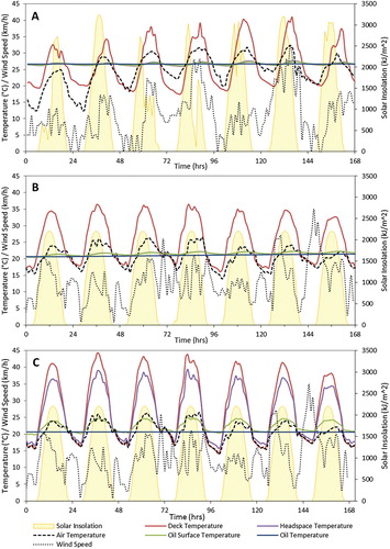
The temperature within the headspace, represented by the average temperature of the plane at a height of 23 m from the bottom of the tank, and the oil surface, represented by the average temperature of the plane at a height of 22 m, are very similar and fluctuate diurnally only slightly, by 1–1.5°C. The temperature in the headspace fluctuates slightly more than the oil surface temperature. The bulk oil temperature represented by the average temperature of the plane at 10 m height, fluctuates only very slightly diurnally by 0.1–0.2°C; as expected given the large mass of oil and insulating effect of the double hull configuration. The average temperature of the oil has a very slight upward trend over the course of the week indicating that steady state is yet to be reached with the given climatic conditions. Vancouver shows a greater increase as the initial temperature of the oil coming from the storage tanks was assumed to be lower due to a lower average July temperature in Vancouver than Montreal.

The oil surface and VOC headspace temperature average trends are higher, increasing by 0.3 and 2°C for Montreal and Vancouver conditions respectively, indicating a faster temperature rise and increasing temperature gradient within the tank.

The large mass of oil in the tank keeps the temperature relatively stable over the week simulated. Heat loss to the relatively cool water surrounding the tanker nearly offsets the heat influx to the tanker deck during daytime heating. In the case of crude oil tanker in Montreal metrological conditions the bulk temperature of the oil decreased by 0.001°C during the simulated week. The crude oil tank configuration in the Vancouver metrological scenario showed an increase in the bulk oil temperature of 1.21°C, due to the lower assumed initial temperature. The oil bulk in the barge tank configuration in Vancouver metrological conditions showed a decrease in temperature of 0.015°C, despite having only 5% the volume of the cargo tanker. This is due to increased heat loss to the surrounding water of the barge tank as the double-wall width is smaller in the barge tank and the overall surface are to volume ratio of the tank is significantly higher.

The diurnal fluctuations in oil surface temperature were greatest in the barge tank configuration at 5.1°C as compared to 1.3°C for the product tanker tank configuration. This is due to the reduced height of the headspace for an equivalence filling ratio of the two tanks.

3.2. Temperature distribution in the tank

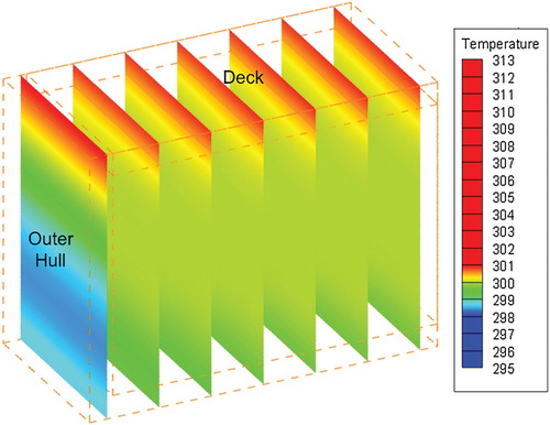
Temperature profiles were generated from the heat transfer simulations. Figure 4 shows the temperature distribution for the Montreal simulation at a time of 139 h, near the peak deck temperature as shown in Figure 3. It can be seen that the deck temperature is significantly higher than the rest of the tank due to solar insolation and high external temperature. The temperature within the air hull is lower than in the oil. The temperature within the bulk oil is nearly uniform, but the temperature within the VOC and air hull has a comparatively large temperature gradient due to the low conduction heat transfer. Results show that the double air hull provides very good thermal stability for the oil.

Figure 4. Tank temperature distribution at time 139 h.

3.3. Effect of main meteorological data on steady temperature distribution

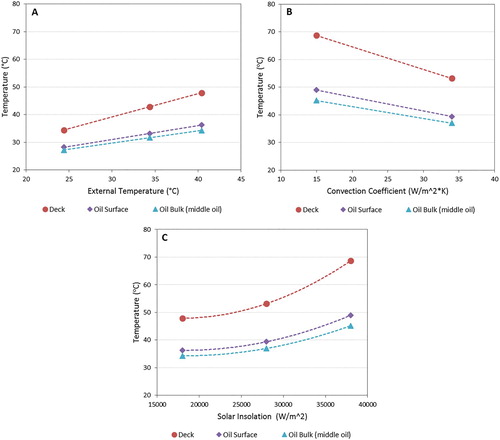
Eight simulations were run with until steady state conditions were reached to determine their effect. Figure 5 shows the effect of the key dependent parameters of external temperature, convection coefficient (wind speed) and solar insolation, on the tank temperatures at steady state. The base conditions (left most points on Figure 5(A)) correspond to Montreal, July metrological conditions. The simulations for different convection coefficients and solar insolation values were conducted at the highest external temperature. The external temperature and solar insolation have a positive effect on the tank temperatures with the magnitude of the effect greater for solar insolation. A solar insolation of 28,000 W/m² is approximately what would be experienced in the US gulf coast. The convection coefficient had a negative relationship with the tank temperatures, with increasing convection leading to lower temperatures in the tank despite using an external temperature of 40°C in these simulations.

Figure 5. Effect of external temperature (A), convection coefficient (B) and solar insolation (C) on oil surface, oil bulk and deck temperature.

3.4. Mass transfer model results

Out of the 8 scenarios simulated, only two resulted in the pressure rising above the release pressure. This is likely the result setting the gas/liquid system to equilibrium initially following loading, an assumption taken based on previous results (Rudd & Hill, 2001). This limited the pressure rise in the tank to the increase in moles evaporated due to the diurnal temperature fluctuations. Table 2 shows the eight scenarios simulated in the mass transfer model and the release events that occurred including the mass of VOCs released and the resulting emissions factors. The first scenario utilized the VOC average temperature profile from the heat transfer simulations which gave a higher maximum temperature (32°C versus 28°C) and greater fluctuation (8.7°C versus 1.0°C).

Table 2. Release events for each scenario and resulting emission factors.

	Metrological Conditions	Temperature Profile	Oil	Release Events	Time of Release (hr)	Mass of VOCs (kg)	Emission Factor (mg/L/day)
1	Montreal Summer	VOC Avg.	CLB	1	19	62.8	10
2	Montreal Summer	Surface	CLB	None	–	–	–
3	Montreal Summer	Surface	MSC	1	7	128.8	21
4	Vancouver Summer	Surface	MSC	None	–	–	–
5	Vancouver Summer	Surface	CLB	None	–	–	–
6	Vancouver Summer	Barge Surface	CLB	None	–	–	–
7	Vancouver Summer	Surface	Gasoline	None	–	–	–
8	Vancouver Summer	Barge Surface	Gasoline	None	–	–	–

CLB: Cold Lake Blend, MSC: Mixed Sweet Crude.

As expected, the higher temperature profile (VOC average) used in the mass transfer model results in a faster volatilization, increased pressure due to increase in moles of gas and a release event for the low volatility crude oil CLB, whereas the surface temperature profile and CLB crude did not have a release event, as seen in scenarios 1 and 2 in Table 2.

The CLB showed less volatility and there were no release events for this crude and the surface temperature profiles (scenarios 2–6); however, the MSC had a single release event during Montreal metrological conditions (scenario 3). This is due to the higher concentration of C2 – C4 VOCs dissolved in the MSB crude oil compared to CLB, shown in Table 1. As expected the lighter, more volatile compounds were present in a higher concentration than less volatile compounds. Despite having a large amount of C5 – C9 compounds from the addition of the condensate, the CLB has very small amounts of C2 – C4 compounds, as a result of the unconventional surface or steam-assisted gravity drainage (SAGD) mining of the oil sands. As can be seen in Table 3, C5 and lighter compounds form the majority of the VOC emissions, so crudes higher in these compounds will have higher transit emissions. The crude oil will still contain some dissolved C2 – C4 gases at equilibrium, as seen in Figure 6. BTEX compounds account for only 0.66% and 0.52% of the mass of VOCs released in the release events of scenario 1 and 3 respectively.

Figure 6. Concentrations of major species in gas and liquid phase and tank pressure over one week under Montreal, oil surface temperature profile and MSB crude oil.

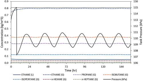
Table 3. Mass of components released during release events and concentrations after 1 week of simulation for different scenarios.

	Scenario
	1	3	2	4	5	6	7	8
Component	Mass at release (kg)		Concentration after 1 week (kg/m^3)
Ethane	0	43.36	0	0.7508	0	0	0	0
Propane	0	15.62	0	0.2552	0	0	0	0
Isobutane	20.07	20.83	0.3188	0.3316	0.2833	0.273	0.271	0.269
N-BUTANE	0	32.12	0	0.5082	0	0	0	0
Isopentane	34.12	6.72	0.5289	0.1046	0.4596	0.441	0.442	0.437
N-Pentane	0	7.15	0	0.1100	0	0	0.0700	0.0692
N-Hexane	6.61	1.73	0.0965	0.0254	0.0795	0.0750	0.0907	0.0894
N-Heptane	1.23	0.44	0.0176	0.0063	0.0143	0.0134	0.0282	0.0278
N-Octane	0.27	0.12	0.0037	0.0016	0.0029	0.0027	0.0069	0.0068
N-Nonane	0.06	0.03	0.0008	0.0005	0.0006	0.0005	0.0006	0.0006
N-Decane	0.009	0.001	0.0001	0	0.0001	0.0001	0.0011	0.0011
Benzene	0.25	0.28	0.0038	0.0043	0.0032	0.0030	0.0016	0.0016
Toluene	0.13	0.28	0.0019	0.0041	0.0016	0.0015	0.0105	0.0103
Ethylbenzene	0.006	0.03	0.0001	0.0003	0.0001	0.0001	0.0012	0.0012
Xylenes	0.03	0.08	0.0004	0.0012	0.0003	0.0003	0.0003	0.0017
Hydrogen sulfide	0	0.001	0	0	0	0	0	0
Ethanol	0	0	0	0	0	0	0.0758	0.0755

When gasoline was used as the cargo, venting did not occur but came close in the shallow draft barge configuration due to the higher temperature reached in the much smaller tank. The ethanol increased the moles of VOC in the headspace, but not beyond the point of venting. The lower temperatures reached in the Vancouver scenario prevented venting from occurring. In Canada, such surface barges are primarily using for transporting refined cargo on the west coast.

In Table 3 it can be seen that the more volatile species dominate the VOCs released and the gas make-up in the tank headspace as expected. The bulk of the ethane present in the MSB crude blend volatilizes into the headspace gas phase and contributes significantly to the release event in scenario 3. This illustrates the need to remove ‘permanent' gases from the crude oil blend prior to loading and transport to minimize or eliminate transit emissions.

Figure 6 shows concentrations of major species in gas and liquid phase and tank pressure over the week of simulation for the first scenario. It is found from the figure that there is one release vent at approximately 8 h. After this first venting event, the concentrations of the volatile species in the liquid and gas phase reached equilibrium and the climatic conditions were insufficient to cause pressure rise above the critical pressure for venting. The tank pressure oscillates diurnally with the oil surface temperature as volatiles transfer between the gas and liquid phase with temperature. There was a slight increase in the average oil surface temperature in the Montreal scenarios over the course of a week, but this was insufficient to increase the pressure above the vent point. The temperature rise is greater in the Vancouver scenarios; however, the overall lower daily high temperature prevents venting, and over the course of the week of simulation the maximum pressure reached in the tank of the crude oil tankers is 105 and 110 kPa for MSB and gasoline cargo respectively. If the pressure trend in the tanker carrying gasoline is extrapolated beyond the week simulated, the critical pressure would be reached after approximately 15 days; however, it is likely that the pressure rise will decrease as the oil temperature approaches its equilibrium with the environmental conditions.

The daily emission factors are relatively small as compared to those suggested by the EPA: 150 mg/L/wk for crude oil (US EPA, 2008). The daily emission values for scenarios 3 and 8 spread out over the simulated week give weekly emission factors of 3 mg/L/wk for crude oil in a tank. The difference is likely due to the conservative nature of the EPA emission factors and the difference in climate between the US and Canada. The EPA emission factors apply to tankers operating in much warmer waters, higher air temperatures and higher solar insolation, such as the Gulf of Mexico where the majority of US tanker operation occurs. In Canadian waters the cold temperatures of the water act to cool the cargo, off-setting a portion of the solar heating. In the Gulf of Mexico, the average coastal water temperature in July is approximately 30°C (NOAA, 2018), which would cause further heating of the cargo and increased venting. The Mixed Sweet Blend contains C2 and C3 compounds which rapidly volatilize and are released as emissions. This rapid volatilization results in a shorter duration before the first and only release event and consequently a lower emission factor. After the release event, the pressure in the tank of Mixed Sweet Crude oil rises higher (∼112 kPa) than that of the tank containing Cold Lake Blend (∼108 kPa), but not to the point of causing a second release. In an environment with higher temperatures, the Mixed Sweet Crude tank is more likely to be pushed to a second release event.

It is recommended that experimental trials be conducted on petroleum tankers operating in Canadian waters to determine Canadian specific emission factors and validate the model presented. In the interim emission factors of 21 and 135 mg/L/day can be used for crude oil and gasoline transit respectively. In the interim, an emission factor of 21 can be used for crude oil transit.

4. Conclusions

Mathematical models were developed to describe heat transfer and mass transfer of petroleum cargos in tanker and barges during transit operations. Accounting for local air and water temperatures, solar radiation, and wind variation with time, a CFD heat transfer simulation was conducted using ANSYS Fluent to obtain the temperature distribution within the tank over the course of one characteristically ‘hot' week in July in Montreal and Vancouver. The VOC emissions of different crude oils, vessels and meteorological conditions were obtained using a mass transfer model developed in MATLAB, utilizing the temperature profiles developed in the CFD model. Emission factors were calculated from the predicted VOC release events, assuming a tank release pressure of 115 kPa.

The heat transfer simulations showed that the bulk oil temperature in the tank remained relatively constant. Bulk cargo temperature trended to a steady state temperature of 25–28°C for the summertime conditions utilized in Montreal and Vancouver. The oil surface temperature is similar to the bulk oil temperature, but increases by 1–2°C due to solar insolation. The deck temperatures oscillate diurnally by 15–20°C. The external temperature and solar insolation have a positive effect on the tank temperatures with the magnitude of the effect greater for solar insolation. The convection coefficient had a negative relationship with the tank temperatures.

The liquid and gas headspace were assumed to be in equilibrium at the start of the mass transfer simulations. Only 3 of 8 scenarios had pressure increases large enough to cause venting of VOC. The Mixed Sweet Blend (MSB) had a higher propensity to vent due to the larger fraction of C2-C4 as compared to the Cold Lake Blend (CLB), despite the presence of diluent in the CLB. C2-C5 compounds constituted the majority of VOCs released from crude oils. The gasoline carrying barge had two release events, and ethanol made up the majority of the VOCs released.

The estimated daily emission factors for MSB was 10 mg/L/day. This is significantly lower than the emission factors suggested by the EPA: 150 for crude oil. The colder climate: colder air temperature, lower solar insolation and significantly lower water temperature, is likely the primary reason for the lower emission factors.

The primary recommendation from this work is to conduct experimental validation of the heat and mass transfer models; alternatively experimental determination of emissions factors to update those of the EPA. Experimental validation of the heat transfer model would require a large scale tank exposed to the elements. The mass transfer model could be experimentally validated using small scale tanks alternately heated and cooled to simulate the temperature profile from the heat transfer model.

Acknowledgements

This research was supported by Environment and Climate Change Canada (ECCC). Special thanks to Monica Hilborn from ECCC for her guidance. The authors would also like to thank China Scholarship Council foundation (201708330014) for offering foundation as visiting scholar at UBC.

Disclosure statement

No potential conflict of interest was reported by the author(s).

References

- Chow, K. (2009). Simulation and analysis of gas freeing of oil tanks. Ph. D Thesis, University of Coventry 235pp.
- Dakhel, A. A., & Rahimi, M. (2004). CFD simulation of homogenisation in large scale crude oil storage tanks. Journal of Petroleum Science and Engineering, 43(3–4), 151–161. doi: 10.1016/j.petrol.2004.01.003
- DeLuchi, M. A. (1993). Emissions from the production, storage, and transport of crude oil and gasoline. Air Waste Management Association, 43, 1486–1495. doi: 10.1080/1073161X.1993.10467222
- Environment Canada. (2018). Historical climate data. Retrieved from http://climate.weather.gc.ca/.
- Ghalandari, M., Shamshirband, S., Mosavi, A., & Chau, K. (2019). Flutter speed estimation using presented differential quadrature method formulation. Engineering Applications of Computational Fluid Mechanics, 13(1), 804–810. doi: 10.1080/19942060.2019.1627676
- Hassanvand, A., Hashemabadi, S. H., & Bayat, M. (2010). Evaluation of gasoline evaporation during the tank splash loading by CFD techniques. International Communications Heat Mass, 37, 907–913. doi: 10.1016/j.icheatmasstransfer.2010.05.011
- Hsieh, C.-C., Babcock, R. W., & Stenstrom, M. K. (1993). Estimating emissions of 20 VOCs I: Surface Aeration. Journal of Environmental Engineering, 119(6), 1099–1106. doi: 10.1061/(ASCE)0733-9372(1993)119:6(1099)
- Karbasian, H. R., Kim, D. Y., Yoon, S. Y., Ahn, J. H., & Kim, K. C. (2017). A new method for reducing VOCs formation during crude oil loading process. Journal of Mechanical Science and Technology, 31(4), 1701–1710. doi: 10.1007/s12206-017-0318-7
- Lee, S., Choi, I., & Chang, D. (2013). Multi-objective optimization of VOC recovery and reuse in crude oil loading. Applied Energy, 108, 439–447. doi: 10.1016/j.apenergy.2013.03.064
- Martens, O. M., Oldervik, O., Neeraas, B. O., & Strøm, T. (2001). Control of VOC emissions from crude oil tankers. Marine Technology, 38(3), 208–217.
- Milazzo, M. F., Ancione, G., & Lisi, R. (2017). Emissions of volatile organic compounds during the ship-loading of petroleum products: Dispersion modelling and environmental concerns. Journal of Environmental Management, 204, 637–650. doi: 10.1016/j.jenvman.2017.09.045
- NOAA. (2018). Water temperature table of all coastal regions. Retrieved from https://www.nodc.noaa.gov/dsdt/cwtg/all_meanT.html.
- Oldervik, O., Neeraas, B. O., Strom, T., Martens, O. M., & Meek-Hansen, B. (2000). V OC emission control systems for shuttle tankers and floating storage systems (VOCON) – Final Report, MT23 F00–137. Norwegian Marine Technology Institute. Trondheim. 24pp.
- Pasley, H., & Clark, C. (2000). Computational fluid dynamics study of flow around floating-roof oil storage tanks. Journal of Wind Energy and Industrial Aerodynamics, 86, 37–54. doi: 10.1016/S0167-6105(99)00138-5
- Paulauskienea, T., Zabukasb, V., & Vaitiek-unasc, P. (2009). Investigation of volatile organic compound (VOC) emission in oil terminal storage tank parks. Journal of Environmental Engineering and Landscape Management, 17(2), 81–88. doi: 10.3846/1648-6897.2009.17.81-88
- Peress, J. (2001). Estimate storage tank emissions. Chemical Engineering Progress, 97(8), 44.
- Rota, R., Frattini, S., Astori, S., & Paludetto, R. (2001). Emissions from fixed-roof storage tanks: Modeling and experiments. Industrial and Engineering Chemistry Research, 40, 5847–5857. doi: 10.1021/ie010111m
- Rudd, H., & Hill, N. (2001). Measures to reduce emissions of VOCs during loading and unloading of ships in the EU. AEA Technology, prepared for the European Commission, Directorate General – Environment. Retrieved from http://ec.europa.eu/environment/air/pdf/vocloading.pdf.
- Tamaddoni, M., Sotudeh-Gharebagh, R., Nario, S., Hajihosseinzadeh, M., & Mostoufi, N. (2014). Experimental study of the VOC emitted from crude oil tankers. Process Safety and Environmental Protection, 929, 29–937.
- Treybal, R. E. (1980). Mass-transfer operations (3rd ed.). New York: McGraw-Hill Book Company.
- US EPA. (2008). Transportation and Marketing of Petroleum Liquids. Chapter 5.2 in: AP 42, Compilation of Air Pollutant Emission Factors, 5th ed., EPA.
- Weatherstats.ca. (2018). Solar radiation – hourly data. Retrieved from https://montreal.weatherstats.ca & https://vancouver.weatherstats.ca.