Development of an oscillation-based technology for the removal of colloidal particles from water: CFD modeling and experiments

ABSTRACT

Colloidal particles removal from water is a challenge in surface water treatment. Previously, we suggested an original technique for colloidal particles separation from water based on physical flow manipulation by an oscillating device. Laboratory experiments and 2D numerical simulation indicated that this technology enhances colloidal particles grouping and enables their rapid, simultaneous aggregation and sedimentation. The 2D model used in that study was unable to fully elucidate the grouping mechanism, settling pattern, or particle trajectories. Here, we extended the numerical simulation from 2D to 3D and examined the system’s distinctive flow field. The flow field was solved with computational fluid dynamics (CFD) simulations in the commercial ANSYS Fluent code and validated by dye injection experiments. The sedimentation patterns could nicely be explained by the computational results. This explanation was strengthened by two-dimensional population balance model simulations, which showed that particles aggregated in two zones trailing the paddle edges. Additionally, the results indicate significantly higher TKE values and faster upward vertical velocities at the higher oscillating frequency, which explains the different sedimentation patterns and removal efficiencies generated by the different oscillation frequencies. The use of 3D numerical simulations will help to better understand and further optimize this novel technology.

KEYWORDS:

• CFD simulation
• colloidal particles
• oscillation
• grouping
• flocculation
• water treatment

1. Introduction

Clay, silt and mineral oxides are inorganic particulates that are present in natural surface water. Insofar as these particles can (1) provide a safe environment for protozoa, bacteria and viruses, (2) absorb toxic compounds, and (3) have an aesthetic effect on water, e.g. turbidity and color, their removal should be a standard part of water treatment processes (Engineers, 1985; Sartor et al., 1974; Vega et al., 1998). Though the range of particle sizes may span several orders of magnitude, from ∼ 0.001–10 μm, the most challenging ones to remove are composed of stable, negatively charged mineral particles with at least one dimension that is less than 1 μm. Such particles are termed colloidal particles because they are hardly affected by gravitational force, and therefore, they take extremely long times to settle (Letterman & American Water Works Association, 1999). Additionally, they can cause membrane fouling (Wang & Tarabara, 2008).

To facilitate the removal of colloidal particles from water, treatment processes typically start with coagulation/flocculation, a common process train for increasing the tendency of small particles in an aqueous suspension to attach to one other and form settleable aggregates, termed ‘flocs’. The process involves the addition of a coagulant, traditionally Al³⁺ or Fe³⁺, which neutralizes the electric charge of the particles and destabilizes them. The coagulation stage is done by rapid mixing to promote the formation of a maximal number of joints between the coagulant and particles and to form micro flocs. The subsequent flocculation stage is done with gentle mixing to allow the destabilized micro-flocs to form larger aggregates, on the one hand, and to prevent the aggregated micro-flocs from breaking up, on the other hand, due to the shear stresses of the stirring (Hendricks, 2010; Visser, 1995). A sedimentation stage usually follows the flocculation stage to enable quiescent settling of the formed flocs.

The operational parameters for the coagulation/flocculation process are site specific and are determined in a standard laboratory experiment known as a ‘jar test’. The jar test apparatus is composed of six beakers, each with a stirrer that is adjustable to specific stirring velocities according to the different stages. Recently, Halfi et al. (2019) suggested an original technique for colloidal particle separation from water based on flow manipulation by an oscillating device. This technique, which enables simultaneous aggregation and sedimentation in a single reactor, was found to perform better than the traditional mixing-based technology. The present experimental and computational study is a continuation of that previous work (Halfi et al., 2019). In the current study, the flow field in the new system is solved by using 3-D computational fluid dynamics (CFD) simulations, the results of which are compared with those of dye-injection experiments.

Numerous studies were carried out to numerically and experimentally describe the flow regime created by a stirrer in a cylindrical container. The main conclusions of previous studies are summarized below in this introduction. Included in the literature review are works that examined the effects of meshing method, discretization method, turbulence model, mesh refinement, and impeller type on the flow field.

The first step in the study of flocculation processes in mixing tanks is the flow field analysis (Stanley & Smith, 1995). Stanley and Smith (1995) analyzed the turbulent flow in a standard jar test apparatus by using a two-dimensional laser doppler anemometer. They determined the general flow field inside the jar test apparatus, emphasizing the effects of impeller type on the flow field. These effects were later described by Ochieng et al. (2009) and recently studied by Steiros et al. (2017) and Torotwa and Ji (2018). Stanley and Smith (1995) found large circulation patterns both above and below the impeller. A radial flow pattern was found (Holland & Bragg, 2002). In general, the flow pattern depends mainly on the impeller type, but it is also affected by other operating conditions of the stirred tank (Marshall & Bakker, 2004; Rezend, 1996). For example, an axial flow impeller discharges flow radially with low off-bottom clearances and large ratios between the impeller and tank diameters (Rezend, 1996). Another example is combined axial-radial flow driven by an axial flow impeller, which works in laminar conditions (Marshall & Bakker, 2004).

Marshall and Bakker (2004) described the application of CFD to mixing tanks. To mimic the initial conditions used in that study, the transient simulation should be started when the stirrer is at rest. Moreover, they recommend simulating a periodic steady state with the liquid phase only before introducing additional phases (Marshall & Bakker, 2004).

Aubin et al. (2004) studied turbulent stirred tanks with CFD simulations in CFX 4.4. They compared their previous experimental results (Aubin et al., 2001) with CFD results for different meshing methods, discretization methods, and turbulence models. They performed a preliminary mesh independence study with three meshes, including those with 76,000, 155,000, and 350,000 elements. Based on the dependence of the turbulent kinetic energy on the radial coordinate with three meshes, which was computed in the region 5 mm below the impeller (a location characterized by large gradients), they decided to use the medium mesh for the study. In a comparison of the frozen-rotor multiple reference frame (FR-MFR), the circumferential averaging multiple reference frame (CA-MFR), and the sliding mesh (SM) methods, they found that the meshing method influenced the mean radial and axial flow patterns to a small extent. Aubin et al. (2004) also assessed several discretization methods, including first-order upwind differencing (UW), higher-order upwind differencing (HUW), and quadratic upwind differencing (quadratic upstream interpolation for convective kinetics-QUICK). The mean velocities in the radial and axial directions in the vessel were not affected by the discretization method. However, the UW method under-predicted a small vortex underneath the impeller and the dimensionless turbulent kinetic energy (the turbulent kinetic energy divided by the squared velocity of the impeller tip) in comparison with other computational results. Lastly, they also compared the standard k-ε turbulence model with the renormalization group theory (RNG) k-ε turbulence model and found that neither had any significant effect on the mean velocity in the radial or axial direction or on the dimensionless turbulent kinetic energy.

Deglon and Meyer (2006) performed CFD simulations of a stirred tank in Fluent 6 to explore the effects of mesh resolution and the discretization scheme when using the MRF approach and the standard k-ε turbulence model. They compared simulations with four different meshes with 33,000, 230,000, 800,000, and 1,900,000 as the approximate numbers of elements. They also studied several discretization schemes, namely, upwind (UW), central, and QUICK. They found that even with the coarsest mesh, the typical flow pattern in the stirred tank was predicted. However, more complex flow features, such as the vortices that trail the impeller tip, could only be computed with the two finer meshes. They therefore concluded that while the main features of the flow field in stirred tanks can be predicted using relatively coarse meshes, the detection of more subtle flow field phenomena required finer meshes. Thus, very fine meshes and high-order discretization schemes were needed to obtain complete predictions of the turbulent kinetic energy. They also related to the poor predictions of the turbulent kinetic energy obtained when using the standard k-ε turbulence model, a drawback that has been cited often in previously published studies. These predictions may be caused by numerical errors rather than by an inherent problem with the turbulence model itself.

Other investigations of turbulent flow fields in mixing tanks found that a vortex pair appeared along the top and bottom sides of each blade of a Rushton turbine impeller or of a turbine impeller in which the blades extended radially directly from the shaft (Takashima & Mochizuki, 1971; Van't Riet & Smith, 1973, 1975; Winardi & Nagase, 1994).

Wang et al. (2017) argued that the use of CFD in agitated mixing tanks, in which measurements are either difficult or impossible to obtain, provides highly detailed information about the flow field and the local variables of the system. They performed CFD simulations of a liquid–solid mixing tank in ANSYS Fluent 14. In the axial plane, the observed flow pattern through the impeller was axial because each impeller blade was pitched at a 45-degree angle. In the horizontal plane, the flow was mostly tangential, except in the proximity of the wall baffles. The solid particles used in the study of Wang et al. (2017) were relatively large, with diameters of about 3 mm. Increasing impeller rotation speed from 260 rpm to 360 rpm in their simulations suspended the particles that were at the bottom and near the side of the jar. An additional increase in rotation speed to 460 rpm enhanced particle suspension in the tank, where more uniform particle distribution was obtained than at the lower rotation speeds.

The introduction of a colored dye into the agitated tank may facilitate superior flow visualization (Brown et al., 2004). To that end, the use of a tank with a level indicator in the form of a scale attached to the tank wall can provide valuable quantitative information on the observed height of colored dye. In the present study, dye was injected into the agitated tank at measured depths to study the flow patterns and to compare the dye injection results with those of the simulated flow field. Note that in the conventional jar test configuration, particles do not settle, but rather, they remain suspended in the liquid phase as a result of the flow field generated in the jar test configuration. In fact, a similar configuration is used for solid particle fluidization in cylindrical tanks (Marshall & Bakker, 2004; Nagata, 1975). Therefore, separation of the solid particles from the liquid phase requires an additional sedimentation tank.

Bridgeman et al. (2009) thoroughly reviewed CFD studies on flocculation in water treatment. They reported that at that time, although many studies on bulk flow patterns had already been published, these were primarily at the laboratory scale, and few reported multiphase modeling at either the laboratory scale or at full scale. Recently, Oyegbile and Akdogan (2018) compiled and reviewed the state of the art in the experimental and CFD characterization of stirred tanks and agglomeration reactors. In what follows, we review some of the recent CFD studies in this field.

Wu (2012) studied large-scale mixing tanks with side-entering impellers using CFD simulations in ANSYS Fluent 13.0. His comparison of six turbulence models found that they all gave reasonable predictions, within 20% error, of the power number and flow number. The sliding mesh (SM) approach demonstrated an improvement in the predictions of the power number and flow number with respect to the multiple reference frame (MRF) approach. From the analysis of the flow field, he concluded that increasing the horizontal angle between the impeller shaft and the radial direction may cause vortical flow and that decreasing the vertical angle between the shaft and the side wall may prevent solid particle settling.

Gu et al. (2017) suggested a new type of dual punched rigid-flexible impeller for solid–liquid suspension in a stirred tank and compared it with a dual rigid impeller and a dual rigid-flexible impeller of the same size. Performing CFD simulations in ANSYS Fluent 14.5, they employed a multiple reference frame (MRF) approach in which they exploited the standard k-ϵ turbulence model and the Eulerian-Eulerian multiphase model. In their analysis of the flow fields of the three impellers, they found that the dual punched rigid-flexible impeller achieved higher quality of solid particle suspension, expressed in terms of suspension homogeneity, compared with the other two impellers.

He et al. (2018) studied flocculation for drinking water treatment using experiments and CFD simulations to investigate floc growth dependence on baffle width. Using the multiple reference frames (MRF) impeller rotation model and the standard k-ϵ turbulence model in CFD simulations in the commercial code Fluent v6.3.26, they found that different baffle widths caused distinct turbulent flow fields at the same shear rates. These flow fields, they found, were related to how the flocs developed in size and structure. They thus concluded that the optimal baffle width should be a compromise between the size that breaks water flow rotation with the impeller to increase axial flow rate and that at which the formation of a larger dead zone is prevented.

State-of-the-art applications of CFD include its combination with machine learning and its use in the medical sciences. In recent innovative studies, the CFD-machine learning combination was exploited in chemical engineering applications wherein the CFD output data was used both as input and as output for machine learning. Mosavi et al. (2019) modeled a bubble column reactor with four input variables: x coordinate, y coordinate, z coordinate and the superficial air velocity. The output of machine learning was air velocity. They gradually increased the number of outputs from one to four and found good agreement between the ANFIS (machine learning) results and the CFD simulations with four outputs and four membership functions. The combination of CFD and machine learning significantly reduces the computational time.

Although most of the CFD studies have dealt with classical engineering applications, CFD has also been used in the medical sciences, especially where measurements are cumbersome. CFD simulations enable the effects of different variables on fluid flow to be explored. Ghalandari et al. (2019) studied silver nano-particles dispersed in water for the disinfection of a root canal in endodontic treatment. Specifically, they investigated the concentration of the silver nano-particles in the water and the volumetric flow rate of the nanofluid. They recommended that the flow rate be increased from 0.15 mL/s to 0.25 mL/s and that the nano-particle volume concentration be increased from 0.0025 to 0.01 to improve disinfection.

In our previous study (Halfi et al., 2019), a new technology termed ‘grouping’ for simultaneous flocculation and sedimentation was presented. This technology promotes simultaneous flocculation and sedimentation in a single tank and in shorter time than in the conventional jar test configuration. Based on physical flow manipulation by an oscillating device, the grouping technology, in principle, exploits the tendency of particles (and droplets) in an oscillating flow to gather into groups depending on flow and particle characteristics. In this study, it was shown that by using the oscillation technique, 86% and 79% of the suspended particles were removed after only 15 min of flocculation using 20 and 10 mg/L alum, respectively. These results are in contrast to the very low removal observed in the jar test, wherein less than 14% of the suspended particles were removed with similar alum doses. After 30 min of oscillation/stirring, the jar test separated only 18% and 34% of the mineral colloids using 10 and 20 mg/L alum, respectively, compared to 90% and 94% separation obtained via the oscillation technique using similar doses (Halfi et al., 2019).

The grouping technique is governed mainly by parameters such as the frequency and amplitude of the velocity oscillations, fluid viscosity and particle size (Katoshevski et al., 2005). Initially shown in several experiments and numerical studies (e.g. some are listed in Katoshevski et al., 2005) on gas flows, particles were observed to accommodate to the oscillating gas flow by forming separate clusters traveling at a constant velocity equal to the phase velocity (U_w) with a tendency for smaller particles to form more stable groupings. Mathematical analyses of aerosol particle/droplet dynamics in periodically changing particle-laden flows with nonzero mean velocity were presented in several publications (Katoshevski, 2006; Katoshevski et al., 2005, 2008).

The grouping phenomenon was also observed in a field study conducted on the North Sea coast in Germany where suspended particle matter (SPM) was found to group into a unique pattern of ‘turbidity clouds’ as a result of the oscillations generated by the tidal bores (Winter et al., 2007). A numerical model based on the mathematical analyses was developed to simulate particle grouping, and based on the flow characteristics of the tidal bores, it showed that the stability of the turbidity clouds clearly depended on the amplitude of current velocity oscillations and their frequencies.

In the present study, the flow field in the grouping system was studied by extending the numerical model from 2D to 3D by using CFD simulations and experiments in which dye was injected into the oscillating system. Our development of the 3D model was done to elucidate and quantify the mechanism that generates the simultaneous aggregation and sedimentation observed in the system. In addition, the 3D flow field was examined for different operational conditions in terms of the velocity vector's magnitude, directionality and turbulent kinetic energy to try to understand the unique settling pattern generated under the different operational conditions.

2. Methods

2.1. The oscillator

Original machinery was assembled to examine the aggregation and sedimentation that are generated by the distinctive flow field created by the oscillating flow. This assembly enables one to obtain controlled and accurate oscillating motion with an extensive range of frequencies, amplitudes and wave forms. Therefore, the system can be well optimized and compared with numerical models.

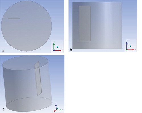
A detailed description of the oscillator assembly can be found in Halfi et al. (2019). The paddle location inside the computational jar is presented in Figure 1. Preliminary experimental results showed that the paddle, whose length is about one half that of the jar’s radius, should not be centered along the jar’s diameter but rather, that it should be centered along the radius.

Figure 1. (a) Top view, (b) side view and (c) 3D view of paddle location in the computational beaker of the oscillator. The diameter of the beaker is 13 cm, the height of the beaker is 12.3 cm, the height of the paddle is 9.3 cm and the distance of the paddle from the water surface and from the bottom of the beaker is 1 and 2 cm respectively.

2.2. CFD modeling

In the present study, the continuity equation, the three-dimensional Reynolds-averaged Navier-Stokes equations and the standard k-ε turbulence model equations were solved (Alfonsi, 2009; ANSYS Fluent, 2015a; Bird et al., 2002; Biswas & Eswaran, 2002; Kundu & Cohen, 2002; Versteeg & Malalasekera, 2007).

2.2.1. Flow equations

The continuity equation for constant density is given by: (1) $\mathrm{\nabla }\cdot \overline{\overrightarrow{v}}=\frac{\mathrm{\partial }\overline{v_x}}{\mathrm{\partial }x}+\frac{\mathrm{\partial }\overline{v_y}}{\mathrm{\partial }y}+\frac{\mathrm{\partial }\overline{v_z}}{\mathrm{\partial }z}=0$(1) where v is velocity, and the overbar denotes the Reynolds average.

The momentum conservation equations for constant density and viscosity for the carrying flow in Cartesian coordinates can be written in vector-tensor form as (Bird et al., 2002): (2) $\frac{\mathrm{\partial }}{\mathrm{\partial }t}\rho \overline{\overrightarrow{v}}=-\mathrm{\nabla }\overline{p}-\left[\mathrm{\nabla }\cdot \rho \overline{\overrightarrow{v}}\overline{\overrightarrow{v}}\right]-\left[\mathrm{\nabla }\cdot \left({\overline{\tau }}^{\left(v\right)}+{\overline{\tau }}^{\left(t\right)}\right)\right]+\rho \overrightarrow{g}$(2) where t is time, ρ is the density, p is pressure, g is the gravitational acceleration, ${\overline{\tau }}^{\left(v\right)}$ is the time-smoothed viscous momentum flux tensor and ${\overline{\tau }}^{\left(t\right)}$ is the turbulent momentum flux tensor (usually referred to as the Reynolds stress tensor).

2.2.2. Turbulence Modeling

The transport equations for the turbulent kinetic energy k and the turbulent dissipation rate ε in the standard k-ε model are given by: (3) $\frac{\mathrm{\partial }\left(\rho k\right)}{\mathrm{\partial }t}+\mathrm{\nabla }\cdot \left(\rho k\overline{\overrightarrow{v}}\right)=\mathrm{\nabla }\cdot \left[\left(\mu +\frac{{\mu }_t}{{\sigma }_k}\right)\mathrm{\nabla }k\right]+P_k-\rho \epsilon$(3) and (4) $\begin{array}{rl}& \frac{\mathrm{\partial }\left(\rho \epsilon \right)}{\mathrm{\partial }t}+\mathrm{\nabla }\cdot \left(\rho \epsilon \overline{\overrightarrow{v}}\right)\\ & =\mathrm{\nabla }\cdot \left[\left(\mu +\frac{{\mu }_t}{{\sigma }_{\epsilon }}\right)\mathrm{\nabla }\epsilon \right]+C_{1\epsilon }\frac{\epsilon }{k}{P}_k-C_{2\epsilon }\rho \frac{{\epsilon }^2}{k}\end{array}$(4) where P_k is the production term of turbulent kinetic energy.

The turbulent viscosity by the standard k-ε model is given by: (5) ${\mu }_t=\rho C_{\mu }{k}^2/\phantom{k^2\epsilon }\epsilon$(5) The standard k-ε model constants are given by: (6) $\begin{array}{rl}{C}_{\mu }& =0.09,C_{\mu }=0.09,{\sigma }_k=1.00,{\sigma }_{\epsilon }=1.30,C_{1\epsilon }\\ & =1.44,C_{2\epsilon }=1.92\end{array}$(6) In the k-ϵ model, with constant density and viscosity, the Boussinesq hypothesis is used to relate the Reynolds stresses to the mean velocity gradient by: (7) $-{\tau }_{ij}=-\rho \overline{{v^{\mathrm{\prime }}}_i{v^{\mathrm{\prime }}}_j}={\mu }_t\left(\frac{\mathrm{\partial }{v}_i}{\mathrm{\partial }{x}_j}+\frac{\mathrm{\partial }{v}_j}{\mathrm{\partial }{x}_i}\right)-\frac{2}{3}\rho k{\delta }_{ij}$(7) where δ_ij is the Kronecker delta function.

2.2.3. Spatial and Temporal discretization

The CFD simulations were performed in the finite volume commercial code ANSYS Fluent with the pressure-based solver. The pressure-velocity coupling method used was ‘Coupled’. The pressure-based coupled algorithm simultaneously solves a coupled system of equations that include the momentum equations and the pressure-based continuity equation. In contrast, the segregated algorithm proceeds sequentially, first solving the momentum equations one after another and then solving the pressure correction equation (ANSYS Fluent, 2015a). The spatial discretization methods were as follows. The least-square cell-based method was used for gradient evaluation. The convection methods we used were second-order for pressure, second-order upwind for momentum, and first-order upwind for turbulent kinetic energy and turbulent dissipation rate. The diffusion terms were central-differenced and second-order accurate.

The time step was 5·10⁻⁴ s for 0.5 Hz and 2.5·10⁻⁴ s for 1 Hz. The time step should meet an important criterion of the overset mesh, namely, that overset mesh movement during one time step should be less than the smallest cell in the overlapping zone (CD-adapco, 2013). With a frequency of 0.5 Hz, the maximal paddle velocity was 0.0628 m/s. Multiplied by the respective time step, this paddle velocity yielded movement of 3.14·10⁻⁵ m. The height of the first layer in the inflation layer (adjacent to the paddle), which represented the smallest cell size, was 7.08·10⁻⁵, which shows that the overset mesh criterion was met. For the frequency of 1 Hz, the maximal velocity was doubled. Therefore, the time step was halved to ensure that the criterion was met for the higher frequency.

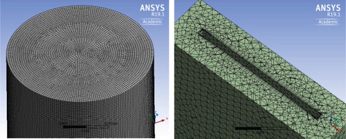
The CFD simulations of the water tank with the oscillator were performed with the overset mesh method in which the mesh used contained 496,678 elements (Figure 2). Of these, 200,733 elements were in the volume surrounding the paddle (the component mesh) and the remaining 295,945 elements were in the water tank (background mesh).

Figure 2. Background mesh of the whole water tank (a, left) and component mesh of the volume surrounding the paddle (b, right)

The convergence criterions were based on the global scaled residuals which are given by (ANSYS Fluent, 2015b): (8) $R^{\phi }=\frac{\sum _{cellsP}\left|\sum _{nb}{a}_{nb}{\phi }_{nb}+b-a_P{\phi }_P\right|}{\sum _{cellsP}|a_P{\phi }_P|}$(8) where φ_P is the value of the general variable φ at cell P, a_P is the center coefficient in the conservation equation after discretization, b is the contribution of the constant part of the source term and of the boundary conditions, subscript nb stands for neighboring cells and a_nb is the influence coefficient of the neighboring cell. The convergence target value of the scaled residuals was 10⁻³.

2.4.4. Boundary conditions and initial conditions

A no-slip boundary condition was assumed at the walls of both the water tank and the paddle. Zero velocities are assumed initially.

2.4.5. Population balance model equations for multiphase simulations

Two-dimensional simulations of the water tank with particles were performed by using the Population Balance Model (PBM) as a multiphase model. The main equations of this model are given in this section (ANSYS Fluent, 2015; Xu et al., 2013; Yeoh et al., 2014).

The mass conservation equation for each phase q is given by (q = 1 for water or 2 for particles): (9) $\frac{\mathrm{\partial }}{\mathrm{\partial }t}\left({\alpha }^q{\rho }^q\right)+\mathrm{\nabla }\cdot \left({\alpha }^q{\rho }^q\overline{{\overrightarrow{v}}^q}\right)=0$(9) where ${\alpha }^q$ is the volume fraction of phase q, ${\rho }^q$ is the density of phase q, and ${\overrightarrow{v}}^q$ is the velocity of phase q.

The volume fractions of the phases must satisfy the following condition: (10) $\sum _{q=1}^2{\alpha }^q=1$(10) The momentum conservation equation of phase q is given by: (11) $\begin{array}{rl}& \frac{\mathrm{\partial }}{\mathrm{\partial }t}\left({\alpha }^q{\rho }^q\overline{{\overrightarrow{v}}^q}\right)=-{\alpha }^q\mathrm{\nabla }\overline{p^q}-\left[\mathrm{\nabla }\cdot \left({\alpha }^q{\rho }^q\overline{{\overrightarrow{v}}^q}\overline{{\overrightarrow{v}}^q}\right)\right]\\ & -\left[\mathrm{\nabla }\cdot \left({\alpha }^q{\overline{{\tau }^q}}^{\left(v\right)}+{\alpha }^q{\overline{{\tau }^q}}^{\left(t\right)}\right)\right]+F_{drag}^q\end{array}$(11) where p^q is the pressure of phase q, ${\overline{{\tau }^q}}^{\left(v\right)}$is the viscous momentum flux tensor of phase q, ${\overline{{\tau }^q}}^{\left(t\right)}$ is the turbulent momentum flux tensor, and $F_{drag}^q$ is the drag force on phase q.

The transport equation for the volume fraction of particle size i is given by: (12) $\begin{array}{rl}& \frac{\mathrm{\partial }}{\mathrm{\partial }t}\left({\rho }_s{\alpha }_i\right)+\mathrm{\nabla }\cdot \left({\rho }_s{\alpha }_i\overrightarrow{v}\right)\\ & ={\rho }_s{V}_i\left(B_{ag,i}-D_{ag,i}+B_{br,i}-D_{br,i}\right)\end{array}$(12) where ρ_s is the density of the secondary phase (meaning the particles), α_i is the volume fraction of particle size i (meaning the volume of the particles of size i divided by the volume of the system), V_i is the volume of particle size i, B_ag,i is the birth rate of particles of size i in aggregation, D_ag,i is the death rate of particles of size i in aggregation, B_br,i is the birth rate of particles of size i in breakage and D_br,i is the death rate of particles of size i in breakage.

The solution in ANSYS Fluent is presented by the bin fraction f_i which is the quotient of the bin volume fraction α_i and the particle phase volume fraction α² (the total volume fraction of the particle phase): (13) $f_i=\frac{{\alpha }_i}{{\alpha }^2}.$(13) The volume is discretized by (Hounslow et al., 1988): (14) $V_{i+1}/\phantom{V_{i+1}{V}_i=2^q}{V}_i=2^{q}q=1,2,\dots$(14) where 2q is the ratio factor, and q is the ratio exponent (here it is equal to one).

The rates of particle birth and death by aggregation are given by: (15) $B_{ag,i}=\sum _{k=1}^{N_{bins}}\sum _{j=1}^{N_{bins}}{a}_{kj}{N}_k{N}_j{x}_{kj}{\xi }_{kj}$(15) and (16) $D_{ag,i}=\sum _{j=1}^{N_{bins}}{a}_{ij}{N}_i{N}_j$(16) where a_kj is the aggregation coefficient of particles of bins k and j, N_k is the particle number density of bin k, x_kj is the contribution fraction, and ξ_kj determines whether the aggregate belongs to bin i.

V_ag,kj is the particle volume resulting from the aggregation of particles k and j: (17) $V_{ag,kj}=V_k+V_j$(17) The factor that determines whether the aggregate belongs to bin i is given by: (18) ${\xi }_{kj}=\left\{\begin{array}{ll}1& \text{for}{V}_i\le V_{ag,kj}<V_{i+1}\\ 0& \text{otherwise}\end{array}\right.\begin{array}{c},i\le N_{bins}-1\\ \end{array}.$(18) The contribution fraction is given by: (19) $x_{kj}=\left\{\begin{array}{ll}\frac{V_{i+1}-V_{ag.kj}}{V_{i+1}-V_i}& V_i\le V_{ag,kj}<V_{i+1}\\ \frac{V_{ag}}{V_{N_{bins}}}& V_{N_{bins}}\le V_{ag,kj}\end{array}\right..$(19) The turbulent aggregation coefficient of particles of bins k and j is calculated based on the Kolmogorov microscale, a measure of the size of the smallest eddies (Tennekes & Lumely, 1972): (20) $\eta =({\nu }^3/\phantom{{\nu }^3\epsilon }\epsilon {)}^{1/\phantom{14}4}$(20) where ν is the kinematic viscosity and ε is the turbulent energy dissipation rate.

In the viscous subrange, when particles are smaller than the Kolmogorov microscale, particle collisions are influenced by the local shear in the eddy. The collision rate is calculated based on the work of Saffman and Turner: (21) $a\left(L_i,L_j\right)={\varsigma }_T\sqrt{\frac{8\pi }{15}}\dot{\gamma }\frac{{\left(L_i+L_j\right)}^3}{8}.$(21) Here $\dot{\gamma }$ is the shear rate: (22) $\dot{\gamma }=(\epsilon /\phantom{\epsilon \nu }\nu {)}^{0.5}.$(22) In the inertial subrange, particles are dragged by velocity fluctuations. The aggregation rate is calculated using Abrahamson's model: (23) $a\left(L_i,L_j\right)={\varsigma }_T{2}^{3/\phantom{32}2}\sqrt{\pi }\sqrt{U_i^2+U_j^2}{\left(L_i+L_j\right)}^2/\phantom{{\left(L_i+L_j\right)}^{2}4}4$(23) where $U_i$ is the mean squared velocity for particle i.

The empirical capture efficiency between the colliding particles is calculated by the relationship of Higashitani and colleagues: (24) ${\varsigma }_T=0.732(5/\phantom{5N_T}{N}_T{)}^{0.242};N_T\ge 5$(24) where N_T is the ratio between the viscous force and the Van der Waals force: (25) $N_T=6\pi \mu {\left(L_i+L_j\right)}^3\dot{\lambda }/\phantom{6\pi \mu {\left(L_i+L_j\right)}^3\dot{\lambda }\left(8H\right)}\left(8H\right)$(25) Here H is Hamaker constant of aggregation for kaolin, which is taken as 3.1·10⁻²⁰ (J) (Anderson & Lu, 2001; Novich & Ring, 1984), and $\dot{\lambda }$ is the deformation rate: (26) $\dot{\lambda }={\left(\frac{4\epsilon }{15\pi \nu }\right)}^{0.5}.$(26) The rates of particle birth and death by breakage are: (27) $B_{br,i}=\sum _{j=i+1}^{N_{bins}}g\left(V_j\right)N_j\text{β}\left(V_i|V_j\right)$(27) and (28) $D_{br,i}=g\left(V_i\right)N_i$(28) where $g\left(V_j\right)$ is the breakage frequency, i.e. the fraction of particles of volume V_j breaking per unit time (s⁻¹) and $\text{β}\left(V_i|V_j\right)$ is the probability density function of the breakage of particles from volume V_j to volume V_i.

The Ghadiri breakage model is used to model the solid particle breakage frequency, which depends on the material properties and the impact conditions: (29) $g\left(L_j\right)=K_b{v}^2{L_i}^{5/\phantom{53}3}$(29) where v is the impact velocity and L_i is the particle diameter before breakage. K_b is the breakage constant, which was calculated for kaolin by: (30) $K_b=\frac{{\rho }_s{E}^{2/\phantom{23}3}}{{\mathrm{\Gamma }}^{5/\phantom{53}3}}=3.61\cdot {10}^7$(30) where ρ_s is the particle density, E is the elastic modulus of the granule and Γ is the interface energy (taken for silica in aqueous NaCl solution). The properties were taken from Khaydapova et al. (2015) and Mizele et al. (1985).

The parabolic form of the breakage probability density function is: (31) $\begin{array}{rl}& \text{β}\left(V_i|V_j\right)\\ & =0.5\left[\frac{C}{V_j}+\frac{1-C/\phantom{C2}2}{V_j}\left\{24{\left(\frac{V_i}{V_j}\right)}^2+24\left(\frac{V_i}{V_j}\right)+6\right\}\right].\end{array}$(31) Here C is the shape factor in the range 0 < C < 3.

3. Results and Discussion

This section begins with a description of the experimental observations from a top view of the flow field, following which the 3D CFD simulation results are presented. Next, the results of dye injection experiments are compared with those of the computational results. Afterwards, a comparison of the turbulent kinetic energy and velocity vectors between the different operational conditions is presented. Two-dimensional population balance model simulations are then described. Finally, energy considerations are given. The common goal of the analyses performed herein is to better understand and quantify the unique simultaneous aggregation and sedimentation mechanism of the grouping technique.

3.1. Top-view observation of the flow field

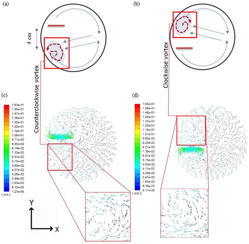
Top-view schematic diagrams based on the experimental observations of the flow field in a water tank with the oscillator show that the length of the path traced by the paddle was shorter than the diameter of the cylinder (Figure 3). Along the cylinder’s perimeter, the water flowed from the paddle zone to the opposite zone, that is, to the other half of the water tank. From there the water flowed toward the inner region of the cylinder (i.e. away from the perimeter of the cylinder) to the oscillator zone of the water tank. The directions of the x and y axes are shown in Figure 3(c and d). The origin of the axes is located in the center of the top base of the cylindrical water tank.

Figure 3. Schematic drawings (a, b) of a top view of the flow field in the water tank with the oscillator when (a) the paddle is at a positive y location and (b) when the paddle is at a negative y location (schematic drawings from Halfi et al., 2019). The blue arrows and the dashed red arrows in panels a and b represent the flow direction and vortices, respectively. (c, d) Comparison with the computational results at a depth of 2 cm, where the zone enveloping the paddle has denser velocity vectors. The arrows are velocity vectors.

3.2. CFD simulation

In the numerical simulation, the flow in the water tank becomes periodical after a few cycles when beginning with quiescent water. At a frequency of 0.5 Hz, each period takes 2 s. The results were taken from 12 s and afterwards, because the flow became periodical at 10 s and because 12 s is the beginning of a new period. The computational results at a depth of 2 cm are shown in Figure 3(c and d), which are comparable to Figure 3(a and b), respectively. The depth of 2 cm was chosen since it is below the upper paddle edge (which is at a depth of 1 cm) and still close to the top of the system.

The computed three-dimensional flow field shows the characteristics that were observed in the experiments: the region of the water tank that contained the oscillator exhibited greater turbulence whereas the other half was quieter. Vortices developed adjacent to the paddle. Along the perimeter, the water flowed from the paddle zone to the opposite zone, meaning to the other region of the water tank. Afterwards, the water flowed internally from the opposite zone of the water tank to the oscillator zone. At the top of the water tank (z = −2 cm, Figure 3), when the paddle was at a positive y location (at 14.25 s, Figure 3(c)), water entered the paddle’s negative y location. At this time and location, the rotational direction of the vortex above the settling zone closest to the tank wall was counterclockwise. At the top of the water tank when the paddle was at a negative y location (at 15.25 s, Figure 3(d)), water entered the positive y location of the paddle. At this time and location, the vortex above the settling zone closest to the tank wall was clockwise. Vortex direction changed when the paddle movement reversed direction. These findings are in agreement with those of the 2D model presented in Halfi et al. (2019). In addition, they also enable the directionality of the vortices to be determined, which shows that they are in agreement with those of the experimental top-view flow field observations (Figure 3(a and b)). The observed changes in vortex direction that accompanied paddle oscillation seem to affect particle sedimentation.

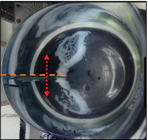
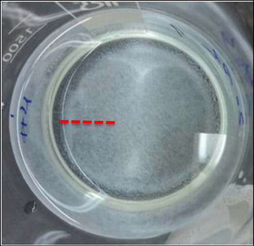
Utilization of the oscillation technique led to the removal of 86% of the suspended particles after only 15 min of oscillations when using 10 mg/L Alum (Halfi et al., 2019). The results of the simulation developed in this work suggest a possible explanation for the sedimentation pattern (Figure 4) that was observed in these experiments: particles are trapped by the vortices adjacent to the paddle in the distinctive flow field that is created by the oscillating paddle, and the trapped particles remain inside the vortices. Vortex velocity is not constant, and it depended on both location and time. Thus, in some regions of the vortices the particles accelerate while in other regions they decelerate, an outcome that results in particle grouping and aggregation and, consequently, their sedimentation. When particles in the vortex accelerate, they catch adjacent decelerating particles downstream. The vortices adjacent to the paddle exist along its entire length, apparently driving a grouping mechanism that is consistent with the findings of the recent study of Dagan et al. (2017). A physical mechanism for the clustering of droplets in vortical flows was described by Bellan and Harstad (1991). In their study, the particles accelerated toward the outer region of the vortex (Bellan & Harstad, 1991), an outcome that resulted in particle cluster formation, grouping of the particles, their aggregation and, consequently, their sedimentation. This finding is in agreement with the observed sedimentation pattern caused by the oscillations (Figure 4), i.e. higher particle concentrations can be seen in the outer region of the pattern.

Figure 4. Top view of particle sedimentation in the experimental beaker. Operational conditions are 0.5 Hz and an amplitude of 20 mm. The dashed line marks the location of the paddle.

The smallest scales present in turbulent flows are known as Kolmogorov microscales (Versteeg & Malalasekera, 2007). The Kolmogorov length microscale was defined above in Eq. 2(2) $\frac{\mathrm{\partial }}{\mathrm{\partial }t}\rho \overline{\overrightarrow{v}}=-\mathrm{\nabla }\overline{p}-\left[\mathrm{\nabla }\cdot \rho \overline{\overrightarrow{v}}\overline{\overrightarrow{v}}\right]-\left[\mathrm{\nabla }\cdot \left({\overline{\tau }}^{\left(v\right)}+{\overline{\tau }}^{\left(t\right)}\right)\right]+\rho \overrightarrow{g}$(2) 0 (Tennekes & Lumely, 1972). In the present study, the maximum computational turbulent dissipation rate was 3.11·10¹ and 1.63·10² (m²/s³), with frequencies 0.5 and 1 Hz, respectively. The resulting Kolmogorov length microscale for water is 1.23·10⁻⁵ and 8.13·10⁻⁶ m, respectively. Based on the average turbulent dissipation rates of 4.80·10⁻⁴ and 3.42·10⁻³ (m²/s³), the average Kolmogorov microscales are 196 and 120 µm, respectively. These scales are significantly larger than the initial particle size, indicating that the particles follow the local water flow (Shamlou, 1993).

Another conjectural mechanism of the observed particle grouping is that it resulted from differences in the drag forces acting on particles of different sizes. Consequently, particles of different sizes exhibited correspondingly different velocities. These differences in particle size and velocity constitute drivers of particle grouping and collisions.

3.3. Model validation by dye injection experiments

The same vortex characteristics were also found in the dye injection experiments. A comparison between the dye injection experiments and the simulation results at a depth of 2 cm showed that the vortices developed and deformed over half a period (Figure 5). The velocity of the dye advance was analyzed with the video images and was estimated to be ∼ 2 cm/s, which is similar to the computed velocity (Figure 5). The counterclockwise vortex along the perimeter grew during paddle acceleration and subsequent deceleration, prior to paddle reversal in direction of motion, and it then deformed as the paddle reached zero velocity. With the reversal in paddle direction, the clockwise vortex began to form and then grew and deformed in the same manner.

Figure 5. (a,b,c,d) Comparison between the dye injection experiments at the top of the water tank and the CFD simulations at a depth of 2 cm. (Note that in this figure the computational graphs are rotated 90° clockwise to facilitate their comparison with the observations of the dye injection experiments.) The zone enveloping the paddle has denser velocity vectors.

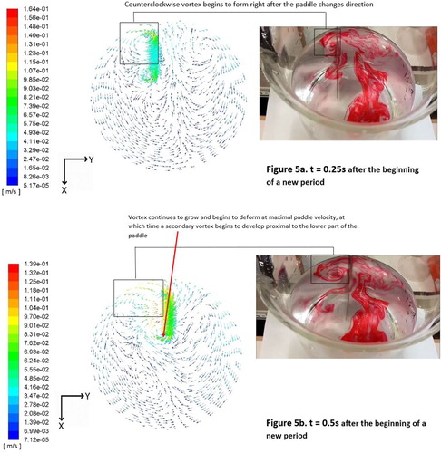
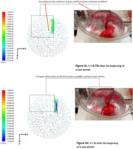
Figure 6(a–c) shows the computational results for other sections of the water tank with the oscillator. Since the flow field is symmetric with respect to the x-axis with a time difference of half a period, only one side of the motion is presented for the planes parallel to the xy plane.

Figure 6. (a,b,c) Computational velocity vectors with the oscillator at 14.25 s in different sections of the water tank at a depth of (a) 5 cm and (b) 9 cm and in the (c) xz vertical plane. The zone that envelops the paddle is that with the densest velocity vectors in (a) and (b) and a dashed line in (c).

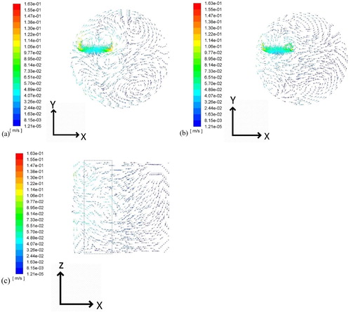
There were two vortices adjacent to the paddle that were rotating in opposite directions. One of these vortices was adjacent to the wall and the other one was closer to the center of the water tank. The vortices adjacent to the paddle reversed their direction during the period. Figures 5–7 demonstrate different depths of the flow field in the water tank with the oscillator. The results indicate not only that the flow field was changing throughout the vertical profile, and therefore, it is three-dimensional, but also that the vortices adjacent to the paddle were similarly extended along the vertical plane.

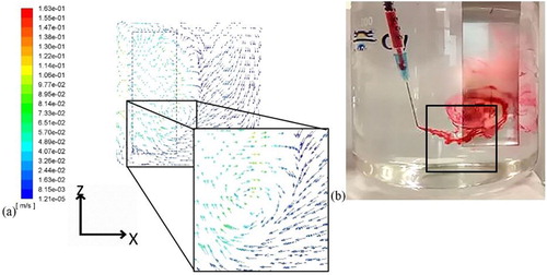
Figure 7 shows a side view of the vectors of the vertical profile in the water tank. A vortex can be seen both in the dye injection experiment and in the calculations of the flow field proximal to the paddle. In the dye injection experiment, this vortex rotated counterclockwise. For the computational results, however, rotational direction was clockwise because the point of view in this case was reversed: the dye injection results were obtained when the paddle was on the right side, whereas for the computational results, the paddle was on the left side.

Figure 7. Comparison between (a) a vortex in the computational velocity vectors in the plane y = 2 cm (parallel to the xz plane) at 14.25 s with (b) a dye injection experiment at a depth of 8 cm.

3.4. Turbulent kinetic energy and velocity vectors – a comparison between two different operational conditions

In Halfi et al. (2019), resuspension was observed when using an oscillating frequency of 1 Hz while virtually no resuspension occurred when the frequency of 0.5 Hz was used. Figure 8(a and b) presents the velocity vectors at a plane located in the middle of the paddle path, meaning x = −3.25 cm. We compared the flow field obtained at these two frequencies.

Figure 8. (a) Computational velocity vectors at an oscillator frequency of 0.5 Hz in the plane x = −3.25 cm at time 18 s. The zone enveloping the paddle has denser velocity vectors. (b) Computational velocity vectors at an oscillator frequency of 1 Hz in the plane x = −3.25 cm at time 7 s. The zone that envelops the paddle has denser velocity vectors.

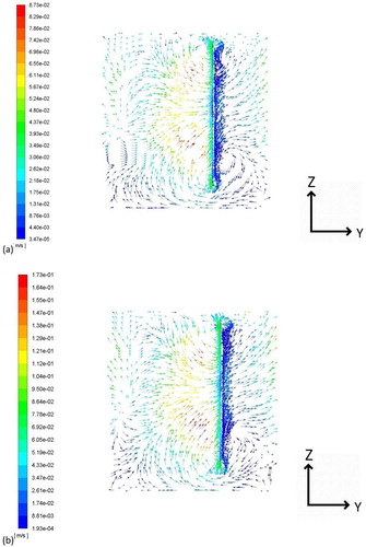
The magnitude of the vertical velocities was greater when using an oscillating frequency of 1 Hz compared to 0.5 Hz. In Figure 8(a), we can see that the maximal vertical velocity is 8.73·10⁻² m/s, whereas in Figure 8(b), it is 1.73·10⁻¹ m/s (red arrows). Furthermore, the direction of the vectors in the bottom right corner of Figure 8(b) are facing upwards in contrast to those obtained for 0.5 Hz in Figure 8(a), which shows that the velocity vectors were mainly oriented toward the bottom of the beaker in this zone.

Figure 9(a and b) compares the turbulent kinetic energy for the frequencies of 0.5 and 1 Hz, respectively. A comparison of Figure 9(a and b) shows significant differences at the two frequencies. For the 0.5 Hz frequency, the zone below the paddle exhibited a region with weak turbulent kinetic energy just above the bottom of the vessel. In contrast, at 1 Hz, the turbulent kinetic energy in the same area of the tank was larger. Additionally, the magnitude of the turbulent kinetic energy generated around the paddle was much higher when using the larger oscillating frequency. The frequency-dependent differences in the turbulent kinetic energy near the bottom of the water tank and around the paddle enabled the particle resuspension observed when using the 1 Hz frequency. The resuspension, in turn, resulted in a uniform sedimentation pattern on the bottom of the beaker (Figure 10) when using high oscillating frequency (1 Hz) in contrast to the distinctive settling zones obtained with the slower oscillating frequency (0.5 Hz) (Figure 4). A mesh independence study for these simulations is presented in the supplementary material (Hedstrom & Osterheld, 1980; Lê et al., 1997).

Figure 9. (a) Computational turbulent kinetic energy with an oscillator frequency of 0.5 Hz in the plane x = −3.25 cm at time 18 s. The white line represents the paddle (side view) and (b) Computational turbulent kinetic energy with an oscillator frequency of 1 Hz in the plane x = −3.25 cm at time 7 s. The white line represents the paddle (side view).

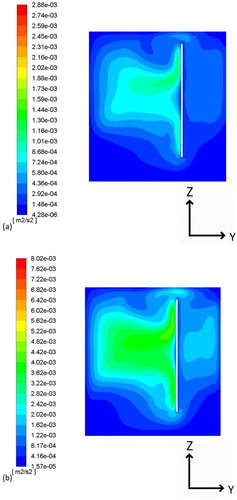
Figure 10. Top view of particle sedimentation patterns when using an oscillating frequency of 1 Hz and an amplitude of 20 mm. The dashed line marks paddle location.

3.5. Two-dimensional population balance model simulations

Population balance model CFD simulations were performed in two dimensions for a cross section of the water tank in the XY plane, without dependence on the Z direction. This simulation utilized dynamic mesh and included 12 bins ranging in size from 1.59 to 20.2 µm. At the beginning of the simulation, all the particles initially belonged to the second bin (from smallest to largest), meaning all the particles had diameters of 2 µm. The time step was 2.5·10⁻⁵ s. The bin fractions f_i (which is the quotient of the bin volume fraction and the particle phase volume fraction) are presented in Figures 11 and 12 together with the velocity vectors.

Figure 11. Bin fractions in the 2D PBM simulation after 0.75 s (a) smallest bin (b) initial bin (c) third bin (d) velocity vectors.

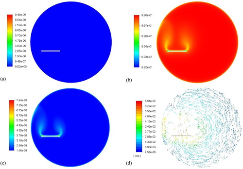
Figure 12. Bin fractions in the 2D PBM simulation after 1.25 s (a) smallest bin (b) initial bin (c) third bin (d) velocity vectors.

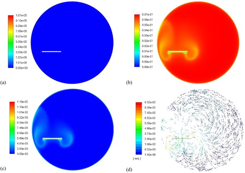
The initial bin is the second smallest in volume and it is adjacent to the smallest bin. Figure 11(a) shows that after 0.75 s of the simulation, the smallest bin fraction is in the range 0–9.49·10⁻⁶, indicating that the particles hardly break. In the initial (second) bin, we can see zones in which the bin fraction decreases, i.e. those following the paddle edges (two yellow stripes in Figure 11(b)) that are located inside the vortices (Figure 11(d)). The third bin, the volume of which is two times that of the initial bin, exhibits increases in the same zones (two green and light blue stripes in Figure 11(c)), indicating that particles of the initial bin aggregated to form the particles of the third bin in these zones. These regions of particle aggregation fit the experimentally observed pattern of particle sedimentation in the water tank. Moreover, they also fit the suggested mechanism of particle grouping: particles are trapped by the vortices adjacent to the paddle, remain inside them, accelerate, decelerate, collide and aggregate. The maximal bin fraction of the fourth bin at this time is 4.23·10⁻⁵.

Figure 12 shows the progress over time of the process depicted in Figure 11. At 1.25 s, the smallest bin fraction is in the range 0–1.01·10⁻⁵, which means that the smallest bin fraction is still practically very small. The particles continue to grow from the initial bin (Figure 12(b)) to the third bin (Figure 12(c)) in curves that follow the paddle and that are located inside the vortices (Figure 12(d)). The maximal fourth bin fraction at this time is 9.49·10⁻⁵.

A mesh independence study for these simulations is presented in the supplementary material.

3.6. Energy considerations

The correlation of Nagata (1975), which was developed for a paddle impeller with two blades, has widespread applicability (Xie et al., 2011). Hiraoka, Kamei, and colleagues suggested another correlation of power for paddle impellers (Furukawa et al., 2012; Hiraoka et al., 2001; Xie et al., 2011). The power consumption of the conventional jar-test configuration was estimated by using both of these correlations, the equations for which are given in the supplementary material. The values obtained via these two methods were 0.256 and 0.297 mW, respectively.

For the oscillator system, the force was calculated by using the Morison equation (Morison et al., 1953) with a hydrodynamic mass coefficient C_m of 0.85 by Sumer and Fredsøe (2006) and mean drag coefficient C_D of 2.0 by Robertson (2016) for rectangular cylinders with low aspect ratios. The Morison equation and the related equations for the power calculation are given in the supplementary material. The mean power computed by the Morison equation was 0.413 mW for a frequency of 0.5 Hz. Compared to the power consumption values obtained for the jar test via the two correlations of Nagata and of Hiraoka, Kamei, and colleagues, that calculated by using the Morison equation is 61.3% or 39.1% larger, respectively. However, for a frequency of 0.3 Hz, which was found to promote colloidal particle aggregation and sedimentation in our previous study (Halfi et al., 2019), the calculated mean power consumption was 0.0891 mW, significantly lower than that of the jar-test, by 65.2% or 70.0%, respectively. Thus, with an energy consumption less than that of the conventional jar-test, the colloidal particle removal efficiency can be increased by the suggested technology.

4. Conclusions, limitations and future studies

The present study focused on the 3D flow field in a new oscillatory system for colloidal particle removal from water. The flow field was solved by using three-dimensional computational fluid dynamics (CFD) simulations. The flow field in the new system was also examined in dye injection experiments at measured depths. Very good agreement was obtained between simulations and experiments in terms of (1) velocity directions in the different zones of the system at different times during the oscillation period, (2) flow patterns, and (3) vortex formation and development.

The simulation results suggest a conjectural explanation for the unique sedimentation pattern observed in the oscillator. The particles, which were trapped by the vortices adjacent to the paddle in the distinctive flow field that was generated by the oscillating paddle, accelerated and decelerated as the vortex velocities changed. This resulted in their grouping, aggregation, and sedimentation. Results of two-dimensional population balance model simulations show that particles aggregated in two zones following the paddle edges, a finding that is in agreement with this conjectural explanation and with the experimental particle settling pattern.

A comparison of the flow fields observed at the different oscillation frequencies found significant differences. In the zone below the paddle, where particle resuspension was observed in the experiments, larger upward velocity and turbulent kinetic energy values were found in the simulations of the higher oscillation frequency. Based on our comparison of the two oscillation frequencies, the simulation results correspond with those from the experiments and explain the different settling patterns that are generated by the different oscillation frequencies. The main limitation of the 3D model is that working with it is time consuming. However, the high level of similarity between the results of the numerical model and those of the dye experiments will enable the system to be further optimized in future works in terms of its oscillating frequency, paddle location and shape, and other operating parameters. For a frequency of 0.3 Hz, which was found to promote colloidal particle sedimentation, the energy consumption was found to be much lower than that of the conventional jar test. Overall, the method presented here is novel and has immense potential as the basis for a more efficient colloidal particle removal process.

Acknowledgements

This study was funded by the Ministry of Science, Technology and Space grant # 3-12586. The authors would like to thank Dr Eduard Moses for his assistance with the ANSYS Fluent software.

Disclosure statement

No potential conflict of interest was reported by the author(s).

Additional information

Funding

This study was funded by The Ministry of Science, Technology and Space: [Grant Number # 3-12586].

References

- Alfonsi, G. (2009). Reynolds-averaged Navier-Stokes equations for turbulence modeling. Applied Mechanics Reviews, 62(4), 040802-1-20. https://doi.org/10.1115/1.3124648
- Anderson, M. T., & Lu, N. (2001). Role of Microscopic Physicochemical forces in large volumetric Strains for Clay Sediments. Journal of Engineering Mechanics, 127(7), 710–719. https://doi.org/10.1061/(ASCE)0733-9399(2001)127:7(710)
- ANSYS Fluent, Advanced add-on modules, Release 16.1. (2015).
- ANSYS Fluent Theory Guide, Release 16.1. (2015a).
- ANSYS Fluent Users Guide, Release 16.1. (2015b).
- Aubin, J., Fletcher, D. F., & Xuereb, C. (2004). Modeling turbulent flow in stirred tanks with CFD: The influence of the modeling approach, turbulence model and numerical scheme. Experimental Thermal and Fluid Science, 28(5), 431–445. https://doi.org/10.1016/j.expthermflusci.2003.04.001
- Aubin, J., Mavros, P., Fletcher, D. F., Bertrand, J., & Xuereb, C. (2001). Effect of axial agitator configuration (up-pumping, down-pumping, reverse rotation) on flow patterns generated in stirred vessels. Transactions of the Institution of Chemical Engineers, 79(Part A), 845–856. https://doi.org/10.1205/02638760152721046
- Bellan, J., & Harstad, K. (1991). The dynamics of dense and dilute clusters of drops evaporating in large, coherent vortices Symposium (International) on Combustion, 23, Elsevier, pp. 1375–1381.
- Bird, R. B., Stewart, W. E., & Lightfoot, E. N. (2002). Transport phenomena (2nd ed.). John Wiley and Sons.
- Biswas, G., & Eswaran, V. (2002). Turbulent flows: Fundamentals, experiments and modeling. Alpha Science International Pangbourne.
- Bridgeman, J., Jefferson, B., & Parsons, S. A. (2009). Computational fluid dynamics modelling of flocculation in water treatment: A review. Engineering Applications of Computational Fluid Mechanics, 3(2), 220–241. https://doi.org/10.1080/19942060.2009.11015267
- Brown, D. A. R., Jones, P. N., Middelton, J. C., Papadopoulos, G., & Arik, E. B. (2004). Chapter 4: Experimental methods. In E. L. Paul, V. A. Atiemo-Obeng, & S. M. Kresta (Eds.), Handbook of industrial mixing: Science and practice (pp. 145–256). John Wiley and Sons.
- CD-adapco. (2013). Best Practices Workshop: Overset meshing. STAR South East Asian Conference 2013, November 11-12. Retrieved from: https://mdx2.plm.automation.siemens.com/sites/default/files/Presentation/Kynan_Overset_Final.pdf
- Dagan, Y., Katoshevski, D., & Greenberg, J. B. (2017). Particle and droplet clustering in oscillatory vortical flows. Atomization and Sprays, 27(7), 629–643. https://doi.org/10.1615/AtomizSpr.2017019152
- Deglon, D. A., & Meyer, C. J. (2006). CFD modelling of stirred tanks: Numerical considerations. Minerals Engineering, 19(10), 1059–1068. https://doi.org/10.1016/j.mineng.2006.04.001
- Engineers, J. M. M. C. (1985). Water treatment principles and design. In Water Treatment Principles and Design (pp. 708–708)
- Furukawa, H., Kato, Y., Inoue, Y., Kato, T., Tada, Y., & Hashimoto, S. (2012). Correlation of power consumption for several kinds of mixing impellers. International Journal of Chemical Engineering, Article ID 106496 (6 pages). https://doi.org/10.1155/2012/106496
- Ghalandari, M., Mirzadeh Koohshahi, E., Mohamadian, F., Shamshirband, S., & Wing Chau, K. (2019). Numerical simulation of nanofluid flow inside a root canal. Engineering Applications of Computational Fluid Mechanics, 13(1), 254–264. https://doi.org/10.1080/19942060.2019.1578696
- Gu, D., Liu, Z., Xie, Z., Li, J., Tao, C., & Wang, Y. (2017). Numerical simulation of solid-liquid suspension in a stirred tank with a dual punched rigid-flexible impeller. Advanced Powder Technology, 28(10), 2723–2734. https://doi.org/10.1016/j.apt.2017.07.025
- Halfi, E., Brenner, A., & Katoshevski, D. (2019). Separation of colloid minerals from water by oscillating flows and grouping. Separation and Purification Technology, 210, 981–987. https://doi.org/10.1016/j.seppur.2018.08.054
- He, W., Xue, L., Gorczyca, B., Nan, J., & Shi, Z. (2018). Experimental and CFD studies of floc growth dependence on baffle width in square stirred-tank reactors for flocculation. Separation and Purification Technology, 190, 228–242. https://doi.org/10.1016/j.seppur.2017.08.063
- Hedstrom, G. W., & Osterheld, A. (1980). The effect of cell Reynolds number on the computation of a boundary layer. Journal of Computational Physics, 37(3), 399–421. https://doi.org/10.1016/0021-9991(80)90045-5
- Hendricks, D. (2010). Fundamentals of water treatment unit processes: Physical, chemical, and biological. CRC Press.
- Hiraoka, S., Kato, Y., Tada, Y., Ozaki, N., Murakami, Y., & Lee, Y. S. (2001). Power consumption and mixing time in an agitated vessel with double impeller. Chemical Engineering Research and Design, 79(8), 805–810. https://doi.org/10.1205/02638760152721613
- Holland, F. A., & Bragg, R. (2002). Fluid flow for chemical engineers (2nd ed.). Oxford Butterworth Heinemann.
- Hounslow, M. J., Ryall, R. L., & Marshall, V. R. (1988). A discretized population balance for nucleation, growth, and aggregation. AIChE Journal, 34(11), 1821–1832. https://doi.org/10.1002/aic.690341108
- Katoshevski, D. (2006). Characteristics of spray grouping/non-grouping behavior. Aerosol and Air Quality Research, 6(1), 54–66. https://doi.org/10.4209/aaqr.2006.03.0005
- Katoshevski, D., Dodin, Z., & Ziskind, G. (2005). Aerosol clustering in oscillating flows: Mathematical analysis. Atomization and Sprays, 15(4), 401–412. https://doi.org/10.1615/AtomizSpr.v15.i4.30
- Katoshevski, D., Shakked, T., Sazhin, S. S., Crua, C., & Heikal, M. R. (2008). Grouping and trapping of evaporating droplets in an oscillating gas flow. International Journal of Heat and Fluid Flow, 29(2), 415–426. https://doi.org/10.1016/j.ijheatfluidflow.2007.10.003
- Khaydapova, D., Milanovskiy, E., & Shein, E. (2015). Rheological properties of different minerals and clay soils. Euroasian Journal of Soil Science, 4(3), 198–202. https://doi.org/10.18393/ejss.2015.3.198-202
- Kundu, P. K., & Cohen, I. M. (2002). Fluid mechanics (2nd ed.). Academic Press Elsevier.
- Lê, T. H., Troff, B., Sagaut, P., Dang-Tran, K., & Phuoc, L. T. (1997). PEGASE: A Navier-Stokes solver for direct numerical simulation of incompressible flow. International Journal for Numerical Methods in Fluids, 24(9), 833–861. https://doi.org/10.1002/(SICI)1097-0363(19970515)24:9<833::AID-FLD522>3.0.CO;2-A
- Letterman, R. D., & American Water Works Association. (1999). Water quality and treatment. McGraw-Hill.
- Marshall, E. M., & Bakker, A. (2004). Chapter 5: Computational fluid mixing. In E. L. Paul, V. A. Atiemo-Obeng, & S. M. Kresta (Eds.), Handbook of industrial mixing: Science and Practice (pp. 257–343). John Wiley and Sons.
- Mizele, J., Dandurand, J. L., & Schott, J. (1985). Determination of the surface energy of amorphous silica from solubility measurements in micropores. Surface Science, 162(1-3), 830–837. https://doi.org/10.1016/0039-6028(85)90986-0
- Morison, J. R., Johnson, J. W., & O’Brien, M. P. (1953). Experimental studies of forces on pile. Proceedings of 4th conference on coastal engineering, Chicago, IL, Chapter 25, 340–370. https://doi.org/10.9753/icce.v4.25
- Mosavi, A., Shamshirband, S., Salwana, E., Chau, K. W., & Tah, J. H. M. (2019). Prediction of multi-inputs bubble column reactor using a novel hybrid model of computational fluid dynamics and machine learning. Engineering Applications of Computational Fluid Mechanics, 13(1), 482–492. https://doi.org/10.1080/19942060.2019.1613448
- Nagata, S. (1975). Mixing principles and applications. John Wiley and Sons.
- Novich, B. E., & Ring, T. A. (1984). Colloid stability of clays using photon correlation spectroscopy. Clays and Clay Minerals, 32(5), 400–406. https://doi.org/10.1346/CCMN.1984.0320508
- Ochieng, A., Onyango, M., & Kiriamiti, K. (2009). Experimental measurement and computational fluid dynamics simulation of mixing in a stirred tank: A review. South African Journal of Science, 105, 421–426.
- Oyegbile, B., & Akdogan, G. (2018). Hydrodynamic characterization of physicochemical process in stirred tanks and agglomeration reactors, Chapter 4. In O. M. Basha & B. I. Morsi (Eds.), Laboratory unit operations and experimental methods in chemical engineering (pp. 57–77). IntechOpen.
- Rezend, C. (1996). CFD analysis of flow field in a mixing tank with and without baffles (Thesis). Rochester Institute of Technology.
- Robertson, F. H. (2016). An experimental investigation of the drag on idealised rigid, emergent vegetation and other obstacles in turbulent free-surface flows (Doctoral dissertation). University of Manchester.
- Sartor, J. D., Boyd, G. B., & Agardy, F. J. (1974). Water pollution aspects of street surface contaminants. Journal (Water Pollution Control Federation), 46(3), 458–467.
- Shamlou, P. A. (1993). Processing of solid-liquid suspensions. Butterworth-Heinemann.
- Stanley, S. J., & Smith, D. W. (1995). Measurement of turbulent flow in standard jar test apparatus. Journal of Environmental Engineering, 121(12), 902–910. https://doi.org/10.1061/(ASCE)0733-9372(1995)121:12(902)
- Steiros, K., Bruce, P. J. K., Buxton, O. R. H., & Vassilicos, J. C. (2017). Effect of blade modifications on the torque and flow field of radial impellers in stirred tanks. Physical Review Fluids, 2(9)), 094802-1-20. https://doi.org/10.1103/PhysRevFluids.2.094802
- Sumer, B. M., & Fredsøe, J. (2006). Hydrodynamics around cylindrical Structures. World Scientific.
- Takashima, I., & Mochizuki, M. (1971). Tomographic observations of the flow around agitator impeller. Journal of Chemical Engineering of Japan, 4(1), 66–72. https://doi.org/10.1252/jcej.4.66
- Tennekes, H., & Lumely, J. L. (1972). A first course in turbulence. MIT Press.
- Torotwa, I., & Ji, C. (2018). A study of the mixing performance of different impeller designs in stirred vessels using computational fluid dynamics. Designs, 2(1), 10. https://doi.org/10.3390/designs2010010
- Van't Riet, K., & Smith, J. M. (1973). The behavior of gas-liquid mixtures near Rushton turbine blades. Chemical Engineering Science, 28(4), 1031–1037. https://doi.org/10.1016/0009-2509(73)80005-3
- Van't Riet, K., & Smith, J. M. (1975). The trailing vortex system produced by Rushton turbine agitators. Chemical Engineering Science, 30(9), 1093–1105. https://doi.org/10.1016/0009-2509(75)87012-6
- Vega, M., Pardo, R., Barrado, E., & Debán, L. (1998). Assessment of seasonal and polluting effects on the quality of river water by exploratory data analysis. Water Research, 32(12), 3581–3592. https://doi.org/10.1016/S0043-1354(98)00138-9
- Versteeg, H. K., & Malalasekera, W. (2007). An introduction to computational fluid dynamics (2nd ed.). Pearson Education Harlow England.
- Visser, J. (1995). Particle adhesion and removal: A review. Particulate Science and Technology, 13(3-4), 169–196. https://doi.org/10.1080/02726359508906677
- Wang, S., Jiang, X., Wang, R., Wan, X., Yang, S., Zhao, J., & Liu, Y. (2017). Numerical simulation of flow behavior of particles in a liquid-solid stirred vessel with baffles. Advanced Powder Technology, 28(6), 1611–1624. https://doi.org/10.1016/j.apt.2017.04.004
- Wang, F., & Tarabara, V. V. (2008). Pore blocking mechanisms during early stages of membrane fouling by colloids. Journal of Colloid and Interface Science, 328(2), 464–469. https://doi.org/10.1016/j.jcis.2008.09.028
- Winardi, S., & Nagase, Y. (1994). Characteristics of trailing vortex (discharged wake vortex) produced by a flat blade turbine. Chemical Engineering Communications, 129(1), 277–289. https://doi.org/10.1080/00986449408936263
- Winter, C., Katoshevski, D., Bartholomä, A., & Flemming, B. W. (2007). Grouping dynamics of suspended matter in tidal channels. Journal of Geophysical Research: Oceans, 112(C8). C08010-1-9. https://doi.org/10.1029/2005JC003423
- Wu, B. (2012). Computational fluid dynamics study of large-scale mixing systems with side-entering impellers. Engineering Applications of Computational Fluid Mechanics, 6(1), 123–133. https://doi.org/10.1080/19942060.2012.11015408
- Xie, M. H., Zhou, G. Z., Xia, J. Y., Zou, C., Yu, P. Q., & Zhang, S. L. (2011). Comparison of power number for paddle type impellers by three methods. Journal of Chemical Engineering of Japan, 44(11), 840–844. https://doi.org/10.1252/jcej.11we115
- Xu, L., Yuan, B., Ni, H., & Chen, C. (2013). Numerical simulation of bubble column flows in churn-turbulent regime: Comparison of bubble size models. Industrial and Engineering Chemistry Research, 52(20), 6794–6802. https://doi.org/10.1021/ie4005964
- Yeoh, G. H., Cheung, C. P., & Tu, J. (2014). Multiphase flow analysis using population balance model: Bubbles, drops and particles. Butterworth-Heinemann.