Comparison of different configurations of aerodynamic braking plate on the flow around a high-speed train

Abstract

End of vehicle streamlined head was selected as the installation location, and aerodynamic behavior of trains with and without braking plates was compared to analyze the formation of the braking force and the evolution of the flow field. An IDDES method based on the SST κ–ω turbulence model was used to investigate the unsteady flow, and the numerical algorithm was validated. Results show that the train aerodynamic drag was significantly increased by opening the braking plates, especially when several braking plates were arranged separately in series on each train car. Furthermore, the effect of the plate installed on the tail car was superior to that of the braking plate on the head car, when only a single braking plate was used. It was also found that both the maximum value of the slipstream and negative pressure close to the braking plate depend on the position and size of the braking plate. The flow field around the lower part of the train was only slightly affected by opening the braking plates, and pairs of vortices over the train appeared when the braking plates were opened, significantly affected both size and position of vortices in the train wake.

KEYWORDS:

• High-speed train
• aerodynamic braking device
• aerodynamic behavior
• aerodynamic drag

Introduction

Brake performance is related to the safe operation of vehicles; as vehicle speeds continue to increase, there is a greater demand for more stringent brake system standards (Niu et al., 2019a; Raghunathan et al., 2002). Some new types of brakes have been proposed, such as disk brakes or regenerative brakes. When the train has to use the emergency brakes, reducing the braking distance as much as possible is key to ensuring the safety of passengers and vehicles. Owing to the successful application of aerodynamic brakes in aircraft, aerodynamic brakes have also been applied to high-speed trains (Agrawal, 1986; Wang et al., 2011). There is a proportional relationship between train aerodynamic drag and the square of the train speed (Baker, 2014; Raghunathan et al., 2002; Schetz, 2001), therefore, higher vehicle speed corresponds to an improved braking effect. Japan is at the forefront of aerodynamic brake engineering for high-speed trains. Before the opening of the Shinkansen line in Hokkaido in 1955, research was conducted into aerodynamic braking, in which a variety of aerodynamic braking plates were developed, and some full-scale vehicle tests were carried out (Takami & Maekawa, 2017; Yoshimura et al., 2000). In recent years, researchers in other countries have also begun to study the aerodynamic braking technology of high-speed trains (Jianyong et al., 2014; Lee & Bhandari, 2018; Puharić et al., 2010). Some tests and simulations show that the brake force of the vehicle is effectively increased by opening the aerodynamic brake. For example, the deceleration caused by the aerodynamic braking of a train passing through a tunnel is 0.2 g (Puharić et al., 2010), and the train’s deceleration can be improved by between 8% and 60% for a train speed between 250 and 500 km/h (Jianyong et al., 2014). Based on the study carried out by Wu et al. (2011), the amplitude of the pressure waves caused by two meeting trains and its complexity are found to increase when opening the braking plates. Gao et al. (2016) found that the relative optimal opening angle should be 75°, based on the analysis of the aerodynamic characteristics and flow field variation of the aerodynamic braking plates with different opening angles.

However, research on the aerodynamic behavior of a train with aerodynamic braking plates has not been comprehensive. The effects of the size and position of the braking plate on the flow field of the braking plate has not been addressed. The scarcity of the research in this field makes investigating this area particularly necessary. In this work, the unsteady aerodynamic behavior of the train with different configurations of aerodynamic braking plates and the flow structure around them are simulated, compared, and analyzed. Numerical simulations, including models, methods, computational domain, grid generation, and data processing are presented in Section 2. A brief introduced on analysis of algorithm validation and grid resolution are presented in Section 3. Results and discussion are presented in Section 4. Finally, Section 5 outlines some conclusions.

Numerical simulation

Models

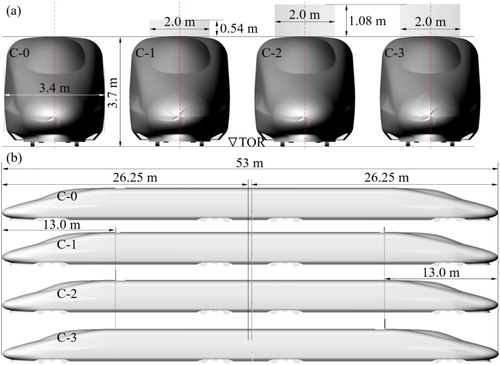
Two types of aerodynamic braking plates, the sizes and shapes of which are presented in Figure 1a, were proposed in this study and were placed in different positions on the top of the train, forming four cases (C-0, C-1, C-2, and C-3). As shown in Figure 1b, these four cases – C-0 (without braking plates), C-1 (with two identical small braking plates installed on the head and tail cars), C-2 (with one large braking plate installed on the head car), and C-3 (with one large braking plate installed on the tail car) are used to study the effect of aerodynamic braking plates on the flow field around the train. The detailed layout, position and size of the braking plate can be found in Figure 1. The train model is consisted of two identical train cars with a streamlined nose, where the total lengths of the train (L_tr) and each car (L_ve) were 53 and 26.25 m, respectively, for the full-scale model. The height (H_tr) – the distance between the train roof and top of rail (TOR) – and width (W_tr) of the train, were 3.7 and 3.5 m, respectively. In order to facilitate the analysis and comparison, braking plates were installed on the top of the train 13 m away from the nose tip.

Figure 1. Front view (a) and side view (b) of the full-scale model of a high-speed train with different aerodynamic braking plate configurations.

Methods

In this study, the Mach number of the incoming airflow is less than 0.3, which means that the airflow around the train can be considered as incompressible. The aerodynamic shape of the train is complex, and the flow field around the train is strongly turbulent and unsteady; therefore, it is important to determine an appropriate turbulence model for obtaining reliable calculation results. Previous studies (Ge et al., 2019; Halila et al., 2019; Issakhov et al., 2019; Li et al., 2018; Menter, 1994; Menter, 1996; Menter et al., 2003; Mou et al., 2017; Niu et al., 2018a; Niu et al., 2019b; Wang et al. 2019a, 2019b) have demonstrated the robustness of the shear-stress transport (SST) κ–ω turbulence model as a means of simulating the strong separation flow; consequently, this model has been widely applied in train aerodynamics (Chen et al., 2018; Chen et al., 2019; Liu et al., 2018;; Niu et al., 2018d; Tschepe et al., 2019; Wang et al., 2018c Wang et al., 2019c; Zhang et al., 2018c). As a hybrid method of RANS/LES, the DES method was proposed in 1997, and the RANS and LES were used to deal with the attached flow and separated flow, respectively (Shur et al., 2008). In practical application, there is a transition region between the two regions simulated by RANS and LES, respectively. This region is neither pure RANS nor pure LES, which leads to some non-physical flow phenomena, such as model stress dissipation (MSD) (Spalart et al., 2006). It will cause grid induced separation (GIS) (Menter & Kuntz, 2004) and log layer mismatch (LLM) (Travin et al., 2002), etc. Therefore, DDES is proposed to solve the problem of GIS (Spalart et al., 2006), then IDDES are proposed to solve the problem of LLM based on DDES (Shur et al., 2008). The idea of these methods is to avoid problems of MSD and GIS by setting an interface in advance (Deck, 2012) by specifying the RANS and DES calculation areas in the flow field. Therefore, IDDES is selected for simulating the aerodynamic behavior of trains. The improved delayed detached eddy simulation method (IDDES) was selected to simulate the flow field in this study as this method combines the advantages of the Reynolds-Averaged Navier-Stokes framework and the Large Eddy Simulation, which have been discussed in detail (Dong et al., 2018; Gritskevich et al., 2012; Zhang et al., 2015). Finally, IDDES with SST κ–ω turbulence model was determined for simulations, and this method has been successfully applied to the simulation of train aerodynamic characteristics by numerous researchers (Chen et al., 2019; Dong et al., 2019; He et al., 2018; Li et al., 2018; Li et al., 2019; Niu et al., 2018b; Tan et al., 2019; Zhang et al., 2019; Zhou et al., 2020).

To realize the accurate simulation of the unsteady aerodynamic characteristics of the train with the aerodynamic braking plate, FLUENT software’s pressure-based solver was used, and pressure-velocity coupling was resolved by the semi-implicit method for pressure-linked equations-consistent (SIMPLEC) (Jang et al., 1986; Latimer & Pollard, 1985; Van Doormaal & Raithby, 1984; Wang et al., 2018a). Convection terms and dissipation terms in equations were dispersed by the bounded central differencing and second-order upwind scheme. To realize the unsteady simulation and ensure that the Courant number was no greater than 1 more than 99% of the computational cells, a dual time-stepping format with second-order accuracy was deal with the time discretisation, and the physical time step was 0.5 × 10⁻⁴ s, no greater than those used in previous studies (Guo et al., 2018; Guo et al., 2019; Maleki et al., 2019; Zhang et al., 2018a). Finally, the residual of each equation could reach up to 10⁻⁵ for each time step.

Computational domain

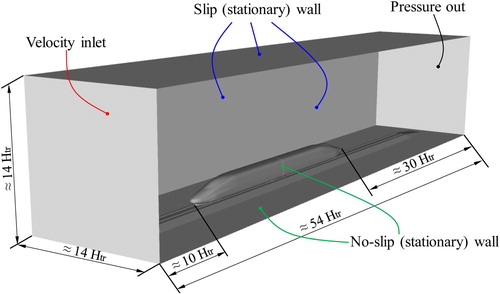
The computational domain was constructed according to the requirements of EN 14067–6 (CEN European Standard, 2010). Its size is presented in Figure 2; the length, width, and height of the computational domain were approximately 54, 14, and 14 H_tr, respectively, and the distances between the front and rear end faces of the computational domain and the train nose were 10 and 30 H_tr, respectively. In order to determine an accurate solution of the flow field, the front and rear end faces of the computational domain were defined as the velocity inlet boundary and pressure outlet boundary, respectively. In order to reduce the disturbance of the boundary layer due to the ground, the lower face of the computational domain was defined as the slipping wall, with the slip velocity as the inflow velocity. The upper face and both sides of the computational domain were defined symmetrically. The incoming flow characteristics was realized by using turbulent kinetic energy κ and specific dissipation rate ω, which can be calculated by Equations (1)–(4) (ANSYS Inc., 2016; Niu et al., 2018a, 2018b; Niu et al. 2019a, 2019b; Russo & Basse, 2016; Turbulence_intensity; Wang et al., 2019b) (1) $\kappa =\frac{\text{3}}{\text{2}}(\text{I}{\text{U}}_{\text{m}}{)}^{\text{2}}$(1) (2) $\omega =\frac{{\kappa }^{\text{1}/\text{2}}}{\text{0}\text{.07}{\text{H}}_{\text{tr},1}{\text{C}}_{\mu }^{1/\text{4}}}$(2) (3) $\text{I = 0}\text{.16R}{\text{e}}^{\text{ - }\text{1}/\text{8}}$(3) (4) $\text{Re}=\frac{\rho {\text{U}}_{\text{m}}{\text{H}}_{\text{tr},1}}{\mu }$(4) where initial air density ρ was 1.225 kg/m³, and empirical constant C_µ was 0.09. Re and I are the Reynolds number and turbulence intensity, respectively, and kinetic viscosity of air µ is 17.9 × 10⁻⁶ Pa·s.

Figure 2. Dimensions of the computational domain and setup of boundary conditions.

Grid generation

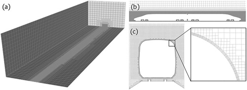
A hexahedral-dominated mesh, widely used in previous studies (Gao et al., 2019; Guo et al., 2020; Salati et al., 2019; Tschepe et al., 2019), was used in grid generation. A refinement box with dimensions of 54 H_tr × 1.5 H_tr × 1.5 H_tr surrounding the train was set to ensure the accurate simulation of the flow field around the train. 10 prism layers were adopted to simulate flow field in the boundary layer, and the distance from core of the initial first boundary layer grid to the train surface is approximately 1.0 × 10⁻⁴ m for the 1: 8 scaled train model. A grid adaptive technology of commercial software FLUENT was applied to keep y+ around the train less than five. An analysis of the train grid independence, including the main subjects of this study, is described in a previous work (Niu et al., 2018c), which evaluated the performance of three types of grid densities (Coarse, Medium, and Fine), used to predict the aerodynamic train characteristics. The maximum aerodynamic drag error for each train car when comparing the Medium and Fine densities was no greater than 1%. There was no obvious difference in the surface pressure of the train among the three grid densities. In this study, the mesh settings of the Medium grid were adopted. The key parameters and the grid around the train that they used are presented in Table 1 and Figure 3 of their paper, respectively (Niu et al., 2018b).

Figure 3. Computational mesh: (a) global view, (b) mesh distribution along the longitudinal section of the computational domain, and (c) mesh distribution around the boundary layers.

Data processing

For the convenience of comparison and analysis in this study, the aerodynamic drag (F_d), aerodynamic lift force (F_l), pressure (p), and slipstream velocity (u) were nondimensionalised via the following: (5) ${\text{C}}_{\text{d(l)}}=\frac{{\text{F}}_{\text{d(l)}}}{\text{0}\text{.5}\rho {\text{U}}_{\text{m}}^{\text{2}}{\text{S}}_{\text{tr}}}$(5) (6) ${\text{C}}_{\text{p}}\text{ = }\frac{\text{p - }{\text{p}}_{\text{0}}}{\text{0}\text{.5}\rho {\text{U}}_{\text{tr}}^{\text{2}}}$(6) (7) ${\text{C}}_{\text{u}}\text{ = }\frac{\sqrt{{({\text{U}}_{\text{m}}-\text{u})}^{\text{2}}\text{ + }{\text{v}}^{\text{2}}+{\text{w}}^{\text{2}}}}{{\text{U}}_{\text{m}}}$(7) where U_m is the velocity of the incoming flow of 60 m/s. S_tr is the cross-sectional area of the uniform train body of 0.175 m² for a 1: 8 scaled model. C_d and C_l are the drag coefficient and lift force coefficient, respectively. C_p and C_u are pressure coefficient and slipstream velocity ratio, respectively. p₀ is the reference pressure at infinity of 0 Pa.

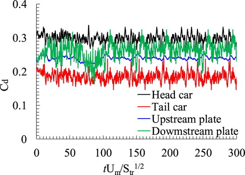
The time-history of the C_d of a train with braking plates in C-1, shown in Figure 4, was taken as an example to introduce the data processing. As demonstrated by the C_d of the train, the curves of C_d were steady, which means that the flow field around the train is fully developed and stable. The data used in nest section were averaged from non-dimensional time tU_m/S_tr^1/2 of 72–287, which is about 14 times the time required for the airflow to pass through the whole train. The sampling time in this study was similar to those used in previous studies (Wang et al., 2017; Wang et al., 2018b; Wang et al., 2019c), and was much longer than those used in (Chen et al., 2018; Dong et al., 2019; Guo et al., 2018; Guo et al., 2019; Li et al., 2019; Wang et al., 2019b).

Figure 4. Time-history of C_d of a train with two small braking plates (C-1).

Verification

Comparison with the vehicle wind tunnel test

Comparisons between numerical calculation results and wind tunnel test data have been conducted previously (Niu et al., 2016; Niu et al., 2017; Niu et al., 2018b; Niu et al., 2018e; Zhang et al., 2018b) and the grid generation and numerical method used in each of these studies are also used in this investigation. The results demonstrate that the maximum error in the aerodynamic drag of the vehicles between the experiment and numerical simulation were 4.02%, according to Niu et al. (2018b), 5.06% according to Niu et al. (2017), and 3% according to Niu et al. (2018c). The pressure distribution along the surface of the vehicles was the same, except for a slight difference between a few measuring points (Niu et al., 2018b). Thus, it is clear that the numerical method used in this study can reliably predict the aerodynamic characteristics of trains.

Comparison with the plate wind tunnel test

The algorithm validation was carried out by some experimental data obtained in a wind tunnel. An introduction to the wind tunnel and test conditions can be found in works by Takami and Maekawa (2017) and Takami (2013). The comparison between numerical simulation and experiment shows that the maximum aerodynamic drag coefficient error between the test and simulation was about 5.15%. More detailed information can be found in Niu et al. (2020).

Finally, the IDDES and related parameter settings used in this study are considered to be reliable, and results calculated by using this calculation method are considered to be accurate.

Results and discussion

Analysis of the unsteady aerodynamic forces

As shown in Table 1, C_d of the head car increased significantly with the opening of the upstream braking plate. The maximum increases in C_d of the head car and tail car can reach a factor of two, which are caused by the opening of the small upstream braking plate and large downstream braking plate, respectively. Taken together, the opening of two small braking plates and a single downstream braking plate exhibit a similar effect in increasing the aerodynamic drag of the entire train, as both increase the aerodynamic drag by approximately 400%, which is nearly 25% larger than that obtained by opening the single large upstream braking plate. An interesting phenomenon here is that the larger braking plate does not necessarily result in a higher aerodynamic drag of the vehicle.

Table 1. Time-averaged aerodynamic forces of each part of the train in different cases.

Case No.	Head car	Tail car	Upstream plate	Downstream plate	Whole
0	0.1006	0.0912	/	/	0.1918
1	0.2966	0.1829	0.2361	0.2500	0.9656
2	0.1468	0.1636	0.4956	/	0.8060
3	0.1067	0.2742	/	0.5648	0.9457
e1(%)	195	101	/	/	403
e2(%)	46	79			320
e3(%)	6	201			393

Analysis of the unsteady flow field around the train

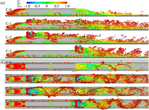
As shown in Figure 5, the flow field around the train was significantly affected by the aerodynamic braking, as many vortices appeared behind the braking plates, and the vortices caused by the large braking plate were larger than those caused by the small braking plate. The vortices in the wake gradually disappeared under the interaction with the upstream vortices produced by the opening of the braking plate. The number of vortices in the wake of the train with two small plates (C-1) s much greater than in the wake of the train with a single plate (C-2 and C-3), and the vortices in the wake of the train with a single large upstream braking plate are also closer to the subgrade, owing to the suppression of the faster upper airflow. Figure 5 shows that vortices generated by the single large upstream plate gradually disappear as they flow to the tail of the train, which results in a significantly smaller number of vortices for C-2 than for the other two cases (C-1 and C-3) with a downstream braking plate. As shown in Figure 5a, small vortices were generated by the small braking plates arranged in series on the roof of the train, large vortices are caused by the large braking plate, which would result in a relatively large vibration of the vehicle and the braking plate, and test the fatigue and installation strength of the braking plate structure. The influence of the layout and configuration of the braking plate on the components of aerodynamic drag (pressure drag and friction drag) will be presented in the future. Figure 5a also shows that the number of vortices in the wake of the train with a braking plate installed on the tail is higher, and the strength greater, than other cases, and combined with the data in Table 1, it is found that the braking plate arranged on the train tail can not only increase the aerodynamic drag, but also enhance the train wake, and further increase the aerodynamic drag. Figure 5b shows that vortices present obvious intermittent shedding from the braking plate and train tail, and theses shedding vortices may cause structural flutter of the braking plate (Ghalandari et al., 2019).

Figure 5. Side (a) and top view (b) of instantaneous iso-surfaces corresponding to the Q criterion (Q = 100 000) for the four cases, rendered by U/U_m, U is the mean velocity.

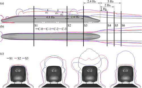
As shown in Figure 6a, the thickness of the boundary layer around the train significantly increases with the opening of the braking plates, and decreases gradually along the train to the downstream area in the larger upstream braking plate case. Meanwhile, the thickness of the boundary layer over the train is always high in the case with two small braking plates. Figure 6a also shows that the maximum value of the boundary layer is evident over the train with different braking plate configurations, with the large upstream braking plate (C-2) having the largest maximum value, the large downstream braking plate (C-3) having a similar, second largest value, and the third largest corresponding to the two small braking plates (C-1). Figure 6b shows that the flow field is less affected by the braking plate on both sides of the train but is more affected by the braking plate in the wake. Figure 6a also shows that differences of the boundary layer profile among these cases are clear. As shown in Figure 6c, the profiles of the boundary layer around the train differ from each other, which reflects the fact that different braking plate configurations have different effects on the aerodynamic performance. Figure 6c clearly shows that the braking plate mainly affects the flow field around the upper part of the train and has a relatively small impact on the lower and middle parts of the vehicle.

Figure 6. 2D boundary layer over the train. (a), (b), and (c) are on the longitudinal plane, horizontal plane, and cross section of the train, respectively.

As shown in Figure 7, three large vortices (V₁,V₂, and V₃) are formed around the braking plate by the recombination of the upstream boundary layer vorticity under the action of the reverse pressure gradient, one of which (V₁) is located upstream of the braking plate, while the other two (V₂ and V₃) are located downstream of the braking plate (the small vortex V₂ is located at the bottom of the braking plate, and the largest vortex V₃ is located far away from the braking plate). The normal pressure gradient of the flow field upstream of the braking plate results in downwash, which induces a large flow shear on the front wall of the braking plate and forms a horseshoe vortex system that includes the clockwise vortex of V₁ and several small vortices around it. Compared with the flow field around the large braking plate and small braking plate, some differences in the shape and location of the V₁ vortex are found, with a smaller V₁ strength around the small braking plates than around the large plates, owing to the change in the height of the braking plate. In this case, the increase in the height of the plate strengthens the upper airflow upstream of the braking plate and suppresses the expansion of the V₁ vortex at the lower part of the airflow upstream of the braking plate. Figure 7a and b show that the V₃ vortex caused by the small upstream plate is farther away (Δx1 > Δx2) and higher (Δy1 > Δy2) than the vortex caused by the small downstream braking plate, which means that V₃ behind the small upstream braking plate is much stronger, owing to the relatively fast airflow separated from above the small upstream braking plate. Inhibition of V₃ pushed away from the braking plate on the development of the V₂ vortex was weakened, which makes V₂ behind the small upstream plate stronger than that behind the small downstream braking plate. Figure 7a and c show that both the strength and height of V₃ are increased by the increase in the height of the braking plate (Δy1 < Δy3), which has little effect on the distance from V₃ to the upstream braking plate in the flow direction (Δx1 ≈ Δx3). Figure 7b and d show that the strength, height, and distance of V₃ to the upstream braking plate in the flow direction are all significantly increased by the increase in the height of the braking plate (Δx2 < Δx4 and Δy2 < Δy4). As depicted in Figure 7c and d, there is little difference in either size or position of V₁ and V₂ between C-2 and C-3; however, there is a significant difference in V₃ between the two cases in that in C-3, V₃ is closer to the braking plate (Δx3 > Δx4 and Δy3 ≈ Δy4). The vortex caused by the upstream braking plate is also found to be larger than that caused by the downstream braking plate.

Figure 7. Mean pressure contour around the train and time-averaged streamlines around the braking plates on the symmetry plane.

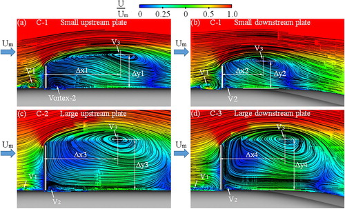
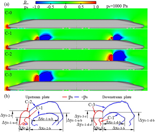
Figure 8a shows how opening the braking plate significantly affects the pressure distribution above the train, especially in the area around the braking plate, and large positive and negative pressures are formed upstream and downstream of the plate, respectively. This is one of the main reasons for the raise in the train aerodynamic drag, while another is the change of the airflow around the train caused by opening the braking plates. Figure 8a also shows that the distribution of the pressure around the braking plates due to opening the braking plates varies depending on the braking plate configurations, which can be clearly observed in Figure 8b. As shown in this figure, by comparing the difference between the isobars around the small and large braking plates, the following relationships can be determined: Δx_C-2-r > Δx_C-1-u-r and Δx_C-2-r > Δx_C-1-d-r, Δy_C-2-b > Δy_C-1-u-b, and Δy_C-3-b > Δy_C-1-d-b, which means that the effect of the large braking plate is significant compared with that of the small braking plate. By comparing the difference between the isobars around the large upstream braking plate and downstream braking plate, the following relationships are found: Δy_C-2-r ≈ Δy_C-3-r, and Δx_C-2-b > Δx_C-3-b. These reflect the fact that the effect of the upstream braking plate is greater than that of the downstream braking plate and they differ somewhat from the relationships of Δy_C-1-u-r > Δy_C-1-d-r, Δy_C-1-u-b < Δy_C-1-d-b, and Δx_C-1-u-b > Δx_C-1-d-b, which compare the isobars around the upstream and downstream braking plates in C-1. This is because the velocity of the airflow around the downstream braking plate is significantly reduced by the upstream braking plate.

Figure 8. Mean pressure contour around the train (a) and time-averaged streamlines around the braking plates on the symmetry plane (b).

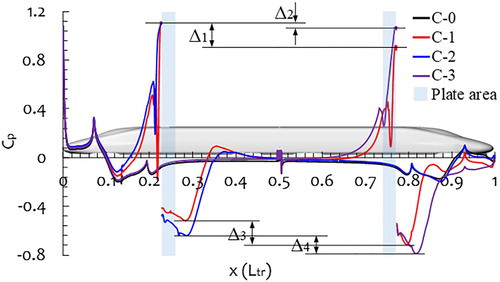
In Figure 8a, the distribution of the mean Cp on the top surface of the train is consistent with the pressure contour. Figure 9a shows that the maximum positive pressure coefficients (C_pmax) of the flow field around the small upstream braking plate (C-1) and around the large upstream braking plate (C-2) are the same, meaning that the maximum positive pressure on the train surface around the upstream braking plate is not affected by the height of the braking plate. Figure 9a also shows that the C_pmax around the large downstream braking plate is a little smaller (Δ₂) than that around the large downstream braking plate; this is because the velocity of the downstream flow filed is relatively low, which is affected by the development of the boundary layer. This phenomenon is more evident in the case with two small braking plates (C-1), with a difference of Δ₁ due to the more significant deceleration of the airflow due to the small upstream plate in front of the small downstream braking plate. With the maximum negative pressure coefficient (−C_pmax), the opposite phenomenon occurs, in which −C_pmax around the downstream braking plate is bigger than that around the upstream braking plate. The −C_pmax on the upper surface of the train behind the braking plate is affected by the height of the braking plate, in which −C_pmax around the braking plate increases with the height of the braking plate. The difference in −C_pmax around the braking plates arranged in series is larger than that for the braking plates arranged separately.

Figure 9. Distribution of time-averaged pressure coefficient along the upper surface of the train.

As shown in Figure 10, abrupt changes occur in the pressure and velocity distributions around the braking plates. The closer to the vehicle, the larger the variation amplitudes of the pressure and slipstream velocity are. Figure 10a shows that the velocity fluctuations caused by the upstream braking plate are greater than those caused by the downstream braking plate owing to the attenuation of the velocity of the downstream airflow, especially for braking plates arranged in series. The velocity field exhibits the opposite behavior, however, as the negative pressure fluctuations caused by the downstream braking plate are much larger than those caused by the upstream braking plate, which can be clearly seen in Figure 10c. Figure 10b and d show that the fluctuations in pressure and velocity of the airflow far away from the vehicle with the braking plates are significantly weaker; the existence of the upstream braking plate weakens the slipstream around the train tail, and the interference range of the large braking plate to the flow field is larger.

Figure 10. Comparison of the distribution of mean C_u (a) and (b) and C_p (c) and (d) along the sampling lines around the high-speed train for four cases: (a) and (c) are along the line at the position of the triangle mark, while (b) and (d) are along the line at the position of the square mark.

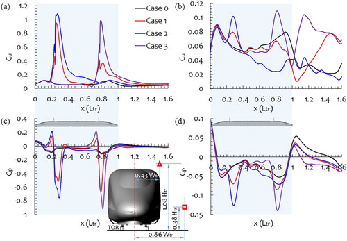
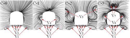
Figure 11 shows that there are always three pairs of vortices under the train (V₂ and V₃) and on both sides of the subgrade (V₁). The size of the V₁ vortex is a little affected by the opening of the braking plate, whereas the other two are not primarily affected. When the braking plate is opened, more vortices (V₄, V₅, and V₆) appear around the vehicle, and there are significant differences in the size and position of the vortices caused by the different braking plate configurations.

Figure 11. Time-averaged flow lines around the tail of the vehicle on the S3 cross-section, which is presented in Figure 6a.

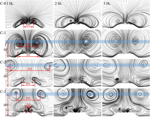
The influence of opening the braking plates on vortices in the wake is discussed in detail here. As shown in Figure 12, the opening of the braking plates induces further vortices, which significantly affect the train wake. As the braking plates are opened, more vortices appear in the wake, and there are significant differences in the height (H₂) and distance (D₂) between the pairs of vortices caused by different braking plate configurations. The vortices produced by the braking plates significantly affect the original vortices in the wake, including their distance (D₁) and position, and the effects caused by the different braking plate configurations are differ significantly from each other. As the distance from the tail of the train increases, D₁ between the pair of vortices increases and their strengths decrease, gradually dissipating.

Figure 12. Time-averaged flow lines in the wake in the different cross-sections – S4, S5 and S6 – presented in Figure 6a.

Conclusion

The aerodynamic behavior of a high-speed train with different aerodynamic braking plate configurations was analyzed and compared, some important conclusions are as follows

1. The aerodynamic drag of the train was significantly increased by the opening of the braking plates. For those cases in which the total windward area of the braking plates is the same, the effect of several braking plates arranged separately in series on each car in the train is better than that of a single braking plate, and the effect of the braking plate installed on the tail car is better than that on the head car.

2. The effect of the single large upstream braking plate (C-2) on the boundary layer over the train is greater than that of the other two cases (C-1 and C-3). The distance from the largest vortex behind the upstream braking plate to the upstream braking plate is greater than that for the downstream braking plate.

3. The maximum value of the slipstream and maximum negative value of the pressure close to the braking plate depends on the position and size of the braking plate; further upstream, the size is larger, and the maximum value of the slipstream is larger. However, for the pressure distribution, there are some differences in the relation – the closer the position is to the downstream, the larger the maximum negative value of the pressure is.

4. The flow field around the lower part of the train is little affected by the opening of the braking plates, and pairs of vortices over the train appear when the braking plates are opened. Both the size and the position of the vortices in the wake of the train are significantly affected by the vortices caused by opening the braking plates.

The research described in this paper focuses primarily on the effects of aerodynamic braking plates on the aerodynamic behavior of the head and tail cars of a train. It is more valuable to study the effect of braking plate configuration on increasing the aerodynamic drag of the middle vehicles, which is also our future work. Because the opening of the braking plate has a significant impact on the aerodynamic performance of the train, the aerodynamic behavior of the train under crosswind is also a key concern, which involves train braking safety.

Acknowledgements

This study was supported by the Fundamental Research Funds for the Central Universities (2682018CX14), the National Natural Science Foundation of China (51805453, 51978575, and 51975487), the Project funded by China Postdoctoral Science Foundation (2019M663551), and the Open Research Project of the National Key Laboratory of Traction Power (TPL1904).

Disclosure statement

No potential conflict of interest was reported by the author(s).

Additional information

Funding

This study was supported by the Fundamental Research Funds for the Central Universities [grant number 2682018CX14], the National Natural Science Foundation of China [grant numbers 51805453, 51978575, and 51975487], the Project funded by China Postdoctoral Science Foundation [grant number 2019M663551], and the Open Research Project of the National Key Laboratory of Traction Power [grant number TPL1904].

References

- Agrawal, S. K. (1986). Braking performance of aircraft tires. Progress in Aerospace Sciences, 23(2), 105–150. https://doi.org/10.1016/0376-0421(86)90002-3
- ANSYS Inc. (2016). ANSYS fluent theory guide, Canonsburg, PA: release 18.0, 2016.
- Baker, C. J. (2014). A review of train aerodynamics part 1–fundamentals. The Aeronautical Journal, 118(1201), 201–228. https://doi.org/10.1017/S000192400000909X
- Chen, G., Li, X. B., Liu, Z., Zhou, D., Wang, Z., Liang, X. F., & Krajnovic, S. (2019). Dynamic analysis of the effect of nose length on train aerodynamic performance. Journal of Wind Engineering and Industrial Aerodynamics, 184, 198–208. https://doi.org/10.1016/j.jweia.2018.11.021
- Chen, Z., Liu, T., Jiang, Z., Guo, Z., & Zhang, J. (2018). Comparative analysis of the effect of different nose lengths on train aerodynamic performance under crosswind. Journal of Fluids and Structures, 78, 69–85. https://doi.org/10.1016/j.jfluidstructs.2017.12.016
- Deck, S. (2012). Recent improvements in the zonal detached eddy simulation (ZDES) formulation. Theoretical and Computational Fluid Dynamics, 26(6), 523–550. https://doi.org/10.1007/s00162-011-0240-z
- Dong, Q. L., Xu, H. Y., & Ye, Z. Y. (2018). Numerical investigation of unsteady flow past rudimentary landing gear using DDES, LES and URANS. Engineering Applications of Computational Fluid Mechanics, 12(1), 689–710. https://doi.org/10.1080/19942060.2018.1510791
- Dong, T., Liang, X., Krajnović, S., Xiong, X., & Zhou, W. (2019). Effects of simplifying train bogies on surrounding flow and aerodynamic forces. Journal of Wind Engineering and Industrial Aerodynamics, 191, 170–182. https://doi.org/10.1016/j.jweia.2019.06.006
- European Standard, C. E. N. (2010). Railway applications-aerodynamics. Part 6: requirements and test procedures for cross wind assessment, CEN EN 14067-6.
- Gao, G., Li, F., He, K., Wang, J., Zhang, J., & Miao, X. (2019). Investigation of bogie positions on the aerodynamic drag and near wake structure of a high-speed train. Journal of Wind Engineering and Industrial Aerodynamics, 185, 41–53. https://doi.org/10.1016/j.jweia.2018.10.012
- Gao, L., Xi, Y., Wang, G., Zhang, P., & Zuo, J. (2016). Opening angle rules of the aerodynamic brake panel. Journal of Donghua University (English Edition), 33(1), 20–24.
- Ge, M., Zhang, H., Wu, Y., & Li, Y. (2019). Effects of leading edge defects on aerodynamic performance of the S809 airfoil. Energy Conversion and Management, 195, 466–479. https://doi.org/10.1016/j.enconman.2019.05.026
- Ghalandari, M., Bornassi, S., Shamshirband, S., Mosavi, A., & Chau, K. W. (2019). Investigation of submerged structures’ flexibility on sloshing frequency using a boundary element method and finite element analysis. Engineering Applications of Computational Fluid Mechanics, 13(1), 519–528. https://doi.org/10.1080/19942060.2019.1619197
- Gritskevich, M. S., Garbaruk, A. V., Schütze, J., & Menter, F. R. (2012). Development of DDES and IDDES formulations for the k-ω shear stress transport model. Flow, Turbulence and Combustion, 88(3), 431–449. https://doi.org/10.1007/s10494-011-9378-4
- Guo, Z. J., Liu, T. H., Chen, Z. W., Xie, T. Z., & Jiang, Z. H. (2018). Comparative numerical analysis of the slipstream caused by single and double unit trains. Journal of Wind Engineering and Industrial Aerodynamics, 172, 395–408. https://doi.org/10.1016/j.jweia.2017.11.022
- Guo, Z., Liu, T., Chen, Z., Xia, Y., Li, W., & Li, L. (2020). Aerodynamic influences of bogie’s geometric complexity on high-speed trains under crosswind. Journal of Wind Engineering and Industrial Aerodynamics, 196, 104053. https://doi.org/10.1016/j.jweia.2019.104053
- Guo, Z., Liu, T., Yu, M., Chen, Z., Li, W., Huo, X., & Liu, H. (2019). Numerical study for the aerodynamic performance of double unit train under crosswind. Journal of Wind Engineering and Industrial Aerodynamics, 191, 203–214. https://doi.org/10.1016/j.jweia.2019.06.014
- Halila, G. L. O., Antunes, A. P., da Silva, R. G., & Azevedo, J. L. F. (2019). Effects of boundary layer transition on the aerodynamic analysis of high-lift systems. Aerospace Science and Technology, 90, 233–245. https://doi.org/10.1016/j.ast.2019.04.051
- He, K., Gao, G. J., Wang, J. B., Fu, M., Miao, X. J., & Zhang, J. (2018). Performance of a turbine driven by train-induced wind in a tunnel. Tunnelling and Underground Space Technology, 82, 416–427. https://doi.org/10.1016/j.tust.2018.08.042
- Issakhov, A., Bulgakov, R., & Zhandaulet, Y. (2019). Numerical simulation of the dynamics of particle motion with different sizes. Engineering Applications of Computational Fluid Mechanics, 13(1), 1–25. https://doi.org/10.1080/19942060.2018.1545253
- Jang, D. S., Jetli, R., & Acharya, S. (1986). Comparison of the PISO, SIMPLER, and SIMPLEC algorithms for the treatment of the pressure-velocity coupling in steady flow problems. Numerical Heat Transfer, Part A: Applications, 10(3), 209–228.
- Jianyong, Z., Mengling, W., Chun, T., Ying, X., Zhuojun, L., & Zhongkai, C. (2014). Aerodynamic braking device for high-speed trains: Design, simulation and experiment. Proceedings of the Institution of Mechanical Engineers, Part F: Journal of Rail and Rapid Transit, 228(3), 260–270. https://doi.org/10.1177/0954409712471620
- Latimer, B. R., & Pollard, A. (1985). Comparison of pressure-velocity coupling solution algorithms. Numerical Heat Transfer, 8(6), 635–652. https://doi.org/10.1080/01495728508961876
- Lee, M., & Bhandari, B. (2018). The application of aerodynamic brake for high-speed trains. Journal of Mechanical Science and Technology, 32(12), 5749–5754. https://doi.org/10.1007/s12206-018-1122-8
- Li, T., Hemida, H., Zhang, J., Rashidi, M., & Flynn, D. (2018). Comparisons of shear stress transport and detached eddy simulations of the flow around trains. Journal of Fluids Engineering, 140(11), 111108. https://doi.org/10.1115/1.4040672
- Li, X. B., Chen, G., Wang, Z., Xiong, X. H., Liang, X. F., & Yin, J. (2019). Dynamic analysis of the flow fields around single-and double-unit trains. Journal of Wind Engineering and Industrial Aerodynamics, 188, 136–150. https://doi.org/10.1016/j.jweia.2019.02.015
- Liu, T., Chen, Z., Zhou, X., & Zhang, J. (2018). A CFD analysis of the aerodynamics of a high-speed train passing through a windbreak transition under crosswind. Engineering Applications of Computational Fluid Mechanics, 12(1), 137–151. https://doi.org/10.1080/19942060.2017.1360211
- Maleki, S., Burton, D., & Thompson, M. C. (2019). Flow structure between freight train containers with implications for aerodynamic drag. Journal of Wind Engineering and Industrial Aerodynamics, 188, 194–206. https://doi.org/10.1016/j.jweia.2019.02.007
- Menter, F. R. (1994). Two-equation eddy-viscosity turbulence models for engineering applications. AIAA Journal, 32(8), 1598–1605. https://doi.org/10.2514/3.12149
- Menter, F. R. (1996). A comparison of some recent eddy-viscosity turbulence models. Journal of Fluids Engineering, 118(3), 514–519. https://doi.org/10.1115/1.2817788
- Menter, F. R., & Kuntz, M. (2004). Adaptation of eddy-viscosity turbulence models to unsteady separated flow behind vehicles. In R. McCallen, F. Browand, & J. Ross (Eds), The aerodynamics of heavy vehicles: Trucks, buses, and trains (pp. 339–352, Vol. 19). Lecture Notes in Applied and Computational Mechanics. Springer.
- Menter, F. R., Kuntz, M., & Langtry, R. (2003). Ten years of industrial experience with the SST turbulence model. Turbulence, Heat and Mass Transfer, 4(1), 625–632.
- Mou, B., He, B. J., Zhao, D. X., & Chau, K. W. (2017). Numerical simulation of the effects of building dimensional variation on wind pressure distribution. Engineering Applications of Computational Fluid Mechanics, 11(1), 293–309. https://doi.org/10.1080/19942060.2017.1281845
- Niu, J., Liang, X., & Zhou, D. (2016). Experimental study on the effect of Reynolds number on aerodynamic performance of high-speed train with and without yaw angle. Journal of Wind Engineering and Industrial Aerodynamics, 157, 36–46. https://doi.org/10.1016/j.jweia.2016.08.007
- Niu, J. Q., Liang, X. F., Zhou, D., & Wang, Y. M. (2018a). Numerical investigation of the aerodynamic characteristics of a train subjected to different ground conditions. Proceedings of the Institution of Mechanical Engineers, Part F: Journal of Rail and Rapid Transit, 232(10), 2371–2384. https://doi.org/10.1177/0954409718770345
- Niu, J. Q., Zhou, D., Liu, T. H., & Liang, X. F. (2017). Numerical simulation of aerodynamic performance of a couple multiple units high-speed train. Vehicle System Dynamics, 55(5), 681–703. https://doi.org/10.1080/00423114.2016.1277769
- Niu, J., Sui, Y., Yu, Q., Cao, X., & Yuan, Y. (2019a). Numerical study on the impact of Mach number on the coupling effect of aerodynamic heating and aerodynamic pressure caused by a tube train. Journal of Wind Engineering and Industrial Aerodynamics, 190, 100–111. https://doi.org/10.1016/j.jweia.2019.04.001
- Niu, J., Wang, Y., Liu, F., & Li, R. (2020). Numerical study on the effect of a downstream braking plate on the detailed flow field and unsteady aerodynamic characteristics of an upstream braking plate with or without a crosswind. Vehicle System Dynamics. https://doi.org/10.1080/00423114.2019.1708959
- Niu, J., Wang, Y., Zhang, L., & Yuan, Y. (2018b). Numerical analysis of aerodynamic characteristics of high-speed train with different train nose lengths. International Journal of Heat and Mass Transfer, 127, 188–199. https://doi.org/10.1016/j.ijheatmasstransfer.2018.08.041
- Niu, J., Wang, Y., & Zhou, D. (2019b). Effect of the outer windshield schemes on aerodynamic characteristics around the car-connecting parts and train aerodynamic performance. Mechanical Systems and Signal Processing, 130, 1–16. https://doi.org/10.1016/j.ymssp.2019.05.001
- Niu, J., Zhou, D., & Liang, X. (2018c). Numerical investigation of the aerodynamic characteristics of high-speed trains of different lengths under crosswind with or without windbreaks. Engineering Applications of Computational Fluid Mechanics, 12(1), 195–215. https://doi.org/10.1080/19942060.2017.1390786
- Niu, J., Zhou, D., Liu, F., & Yuan, Y. (2018d). Effect of train length on fluctuating aerodynamic pressure wave in tunnels and method for determining the amplitude of pressure wave on trains. Tunnelling and Underground Space Technology, 80, 277–289. https://doi.org/10.1016/j.tust.2018.07.031
- Niu, J., Zhou, D., & Wang, Y. (2018e). Numerical comparison of aerodynamic performance of stationary and moving trains with or without windbreak wall under crosswind. Journal of Wind Engineering and Industrial Aerodynamics, 182, 1–15. https://doi.org/10.1016/j.jweia.2018.09.011
- Puharić, M., Lučanin, V., Ristić, S., & Linić, S. (2010). Application of the aerodynamical brakes on trains. Journal of Applied Engineering Science, 8(1), 13–21.
- Raghunathan, R. S., Kim, H. D., & Setoguchi, T. (2002). Aerodynamics of high-speed railway train. Progress in Aerospace Sciences, 38(6–7), 469–514. https://doi.org/10.1016/S0376-0421(02)00029-5
- Russo, F., & Basse, N. T. (2016). Scaling of turbulence intensity for low-speed flow in smooth pipes. Flow Measurement and Instrumentation, 52, 101–114. https://doi.org/10.1016/j.flowmeasinst.2016.09.012
- Salati, L., Schito, P., & Cheli, F. (2019). Strategies to reduce the risk of side wind induced accident on heavy truck. Journal of Fluids and Structures, 88, 331–351. https://doi.org/10.1016/j.jfluidstructs.2019.05.004
- Schetz, J. A. (2001). Aerodynamics of high-speed trains. Annual Review of Fluid Mechanics, 33(1), 371–414. https://doi.org/10.1146/annurev.fluid.33.1.371
- Shur, M. L., Spalart, P. R., Strelets, M. K., & Travin, A. K. (2008). A hybrid RANS-LES approach with delayed-DES and wall-modelled LES capabilities. International Journal of Heat and Fluid Flow, 29(6), 1638–1649. https://doi.org/10.1016/j.ijheatfluidflow.2008.07.001
- Spalart, P. R., Deck, S., Shur, M. L., Squires, K. D., Strelets, M. K., & Travin, A. (2006). A new version of detached-eddy simulation, resistant to ambiguous grid densities. Theoretical and Computational Fluid Dynamics, 20(3), 181–195. https://doi.org/10.1007/s00162-006-0015-0
- Takami, H. (2013). Development of small-sized aerodynamic brake for high-speed railway. Transactions of the Japan Society of Mechanical Engineers Series B, 79(803), 1254–1263. https://doi.org/10.1299/kikaib.79.1254
- Takami, H., & Maekawa, H. (2017). Characteristics of a wind-actuated aerodynamic braking device for high-speed trains. Journal of Physics: Conference Series, 822(1), 012061. IOP Publishing. https://doi.org/10.1088/1742-6596/822/1/012061
- Tan, X. M., Xie, P. P., Yang, Z. G., & Gao, J. Y. (2019). Adaptability of turbulence models for pantograph aerodynamic noise simulation. Shock and Vibration, 2019. https://doi.org/10.1155/2019/6405809
- Travin, A., Shur, M., Strelets, M. M., & Spalart, P. R. (2002). Physical and numerical upgrades in the detached-eddy simulation of complex turbulent flows. In R. Friedrich & W. Rodi (Eds), Advances in LES of complex flows. Fluid mechanics and its applications (pp. 239–254, Vol. 65). Springer.
- Tschepe, J., Fischer, D., Nayeri, C. N., Paschereit, C. O., & Krajnovic, S. (2019). Investigation of high-speed train drag with towing tank experiments and CFD. Flow, Turbulence and Combustion, 102(2), 417–434. https://doi.org/10.1007/s10494-018-9962-y
- Turbulence_intensity. https://www.cfd-online.com/Wiki/Turbulence_intensity.
- Van Doormaal, J. P., & Raithby, G. D. (1984). Enhancements of the SIMPLE method for predicting incompressible fluid flows. Numerical Heat Transfer, 7(2), 147–163. https://doi.org/10.1080/01495728408961817
- Wang, H., Jiang, X., Chao, Y., Li, Q., Li, M., Zheng, W., & Chen, T. (2019a). Effects of leading edge slat on flow separation and aerodynamic performance of wind turbine. Energy, 182, 988–998. https://doi.org/10.1016/j.energy.2019.06.096
- Wang, H., Wang, H., Gao, F., Zhou, P., & Zhai, Z. J. (2018a). Literature review on pressure–velocity decoupling algorithms applied to built-environment CFD simulation. Building and Environment, 143, 671–678. https://doi.org/10.1016/j.buildenv.2018.07.046
- Wang, J., Minelli, G., Dong, T., Chen, G., & Krajnović, S. (2019b). The effect of bogie fairings on the slipstream and wake flow of a high-speed train. An IDDES study. Journal of Wind Engineering and Industrial Aerodynamics, 191, 183–202. https://doi.org/10.1016/j.jweia.2019.06.010
- Wang, S., Avadiar, T., Thompson, M. C., & Burton, D. (2019c). Effect of moving ground on the aerodynamics of a generic automotive model: The DrivAer-Estate. Journal of Wind Engineering and Industrial Aerodynamics, 195, 104000. https://doi.org/10.1016/j.jweia.2019.104000
- Wang, S., Bell, J. R., Burton, D., Herbst, A. H., Sheridan, J., & Thompson, M. C. (2017). The performance of different turbulence models (URANS, SAS and DES) for predicting high-speed train slipstream. Journal of Wind Engineering and Industrial Aerodynamics, 165, 46–57. https://doi.org/10.1016/j.jweia.2017.03.001
- Wang, S., Burton, D., Herbst, A. H., Sheridan, J., & Thompson, M. C. (2018b). The effect of the ground condition on high-speed train slipstream. Journal of Wind Engineering and Industrial Aerodynamics, 172, 230–243. https://doi.org/10.1016/j.jweia.2017.11.009
- Wang, T., Wu, F., Yang, M., Ji, P., & Qian, B. (2018c). Reduction of pressure transients of high-speed train passing through a tunnel by cross-section increase. Journal of Wind Engineering and Industrial Aerodynamics, 183, 235–242. https://doi.org/10.1016/j.jweia.2018.11.001
- Wang, X. L., Wang, F. X., & Li, Y. L. (2011). Aerodynamic characteristics of high-lift devices with downward deflection of spoiler. Journal of Aircraft, 48(2), 730–735. https://doi.org/10.2514/1.C031301
- Wu, M. L., Zhu, Y. Y., Tian, C., & Fei, W. W. (2011). Influence of aerodynamic braking on the pressure wave of a crossing high-speed train. Journal of Zhejiang University-Science A, 12(12), 979–984. https://doi.org/10.1631/jzus.A11GT011
- Yoshimura, M., Saito, S., Hosaka, S., & Tsunoda, H. (2000). Characteristics of the aerodynamic brake of the vehicle on the Yamanashi Maglev test line. Quarterly Report of RTRI, 41(2), 74–78. https://doi.org/10.2219/rtriqr.41.74
- Zhang, J., Wang, J., Tan, X., Gao, G., & Xiong, X. (2019). Detached eddy simulation of flow characteristics around railway embankments and the layout of anemometers. Journal of Wind Engineering and Industrial Aerodynamics, 193, 103968. https://doi.org/10.1016/j.jweia.2019.103968+/7
- Zhang, J., Wang, J., Wang, Q., Xiong, X., & Gao, G. (2018a). A study of the influence of bogie cut outs’ angles on the aerodynamic performance of a high-speed train. Journal of Wind Engineering and Industrial Aerodynamics, 175, 153–168. https://doi.org/10.1016/j.jweia.2018.01.041
- Zhang, J., Wang, X., Liang, D., & Liu, H. (2015). Application of detached-eddy simulation to free surface flow over dunes. Engineering Applications of Computational Fluid Mechanics, 9(1), 556–566. https://doi.org/10.1080/19942060.2015.1092269
- Zhang, L., Yang, M. Z., & Liang, X. F. (2018b). Experimental study on the effect of wind angles on pressure distribution of train streamlined zone and train aerodynamic forces. Journal of Wind Engineering and Industrial Aerodynamics, 174, 330–343. https://doi.org/10.1016/j.jweia.2018.01.024
- Zhang, L., Zhang, J., Li, T., & Zhang, Y. (2018c). A multiobjective aerodynamic optimization design of a high-speed train head under crosswinds. Proceedings of the Institution of Mechanical Engineers, Part F: Journal of Rail and Rapid Transit, 232(3), 895–912. https://doi.org/10.1177/0954409717701784
- Zhou, Z., Xia, C., Shan, X., & Yang, Z. (2020). The impact of bogie sections on the wake dynamics of a high-speed train. Flow Turbulence Combust, 104, 89–113. https://doi.org/10.1007/s10494-019-00052-w