Design optimization and experimental performance test of dynamic flow balance valve

Abstract

This paper considers a solution to the serious problem of hydraulic maladjustment in a dynamic flow balance valve for small diameter and low-pressure drop working conditions. The pressure drop compensation coefficient revising method was proposed to optimize the profile line of the valve core variable opening area. The flow rates of the valve before and after optimization under different displacements were simulated using Computational Fluid Dynamics (CFD) methods. The flow control accuracy of the balance valve before and after the optimization is compared and analyzed to the test values. At the same time, the influence of three key parameters: spring stiffness, the shell structure of the valve core, and geometry imperfections change due to machining burrs on the surface of the valve core for flow control accuracy was discussed. The results show that flow control accuracy after optimization satisfies the requirements of 5% flow rate control. Spring stiffness, the shell structure of the valve core and machining burrs on the surface of the valve core are shown to have an influence on the flow rate of the balance valve. This is especially true for machining burrs which has a larger effect with an average error of 10.1.

KEYWORDS:

• Computational fluid dynamics (CFD)
• design optimization
• flow characteristics
• valves
• flow control accuracy

Introduction

The phenomenon of hydraulic flow imbalance in heating and air-conditioning systems, outdoor heating network systems, and a large number of industrial pipe network systems has always been a significant problem in industry. In order to overcome the impact of hydraulic imbalance at the beginning of the design process, oversized equipment is selected through experience by designers. For example, increasing the head and the water flow rate of the pump is used to compensate for the system hydraulic imbalance. However, as the system size increases a greater emphasis on comfort control and energy cost is required and these methods are found inadequate. Alternately, dynamic flow balance valves are found to be more effective in maintaining flow distribution of hydraulic systems (Cui et al., 2017). Today it is a key self-operated fluid control element for hydraulic flow balance in these systems and plays a critical role in energy conservation and environmental protection (Ryu et al., 2008; Taylor & Stein, 2002).

The dynamic flow balance valve was previously investigated experimentally by a number of researchers. Pietrzak and Witczak (2015) researched air–oil–water flow into a balance valve by testing the flow of the air–oil–water in balanced valves of different sizes, and found that empirical correlation can be used for determining the value of the local pressure drop for the type of valves being investigated. Huovinen et al. (2015) measure the flow rate of the regulating valve by experimental and numerical simulation and showed that, in the case of non-uniformity, the Laser Doppler Velocity (LDV) can be used for volume flow estimation. Sheng et al. (2006) obtained the pressure drop characteristic of the balance valve flow by computational fluid dynamics and experiment. The balance valve is a self-operated fluid control element that is controlled by the coupling of the fluid and the structure. The opening and closing dynamics of the control valve affect the stability of its operation. With the development of computer technology, at present, Computational Fluid Dynamics (CFD) is a significant and convenient calculation method in predicting dynamic characteristics for a valve. Wu et al. (Wu et al., 2015) studied the flow-pressure curve of the pressure regulating valve by numerical simulation method and verified the simulation result through experiments.

They found that this method can deal with changes in operating conditions and varied spring parameters, and that the hydraulic force distribution on the spool is affected by the valve gap and result in pressure loss. The mathematical model of the Pilot-Control Glove Valve (PCGV) was established by Qian et al. (2014). Its dynamic characteristics were simulated by CFD methods. In order to obtain the best design points, they studied the characteristic curve of spool displacement, and concluded that there is a relationship between the static inlet pressure and the spool displacement. Liu et al. (2017) adjust the performance by simulating the flow, and derive the relationship between the flow and the orifice, which is the basis for optimizing the orifice. Aung et al. (2014) present the flow forces and energy loss characteristics in a flapper-nozzle pilot valve with different null clearances by CFD analysis. Cui et al. (2017) used CFD and experimental verification to study the transient flow characteristics of the ball valve at different opening and closing times. To optimize the flow regulating characteristics of the flow regulating valve, Ramanath and Chua (2006) use rapid prototyping (RP) and CFD methods for optimization studies.

In practice, for small diameter products, the flow accuracy control of the dynamic flow balance valve under a small pressure drop cannot meet the requirements of ±5%. The problem of hydraulic imbalance of small caliber dynamic flow balance valves is a serious one in practical applications and causes severe energy loss. Aiming at these problems, this paper proposes a correction method of the pressure drop compensation coefficient based on the motion equation of the valve core. The geometry contour of the variable orifice area is modified and optimized, and the optimization results are verified by numerical simulation. Additionally, a dynamic flow balance flow test bench was established to study the influence of the key parameters of spring stiffness, the structure of the valve core, and machining burrs of the valve core on the accuracy of flow control.

Working principle of the dynamic flow balance valve and design of the valve core

Operating principle

The main components of the balance valve are shown in Figure 1. As seen in the figure, the valve consists of a main body, a core assembly, and a cover. The valve core assembly is the most important part of the balance valve. To make the valve core assembly easy to understand, the other structures were simplified to illustrate the details of the assembly, including the core shell, the core bracket, the spring, the sealing-ring and screw. The balance valve ports are labeled as the inlet port and the outlet port. The inlet port is connected to the upstream main pipeline while the outlet port is often connected to the system end or to the other side of the hydraulic actuator.

Figure 1. Structure of dynamic flow balance valve.

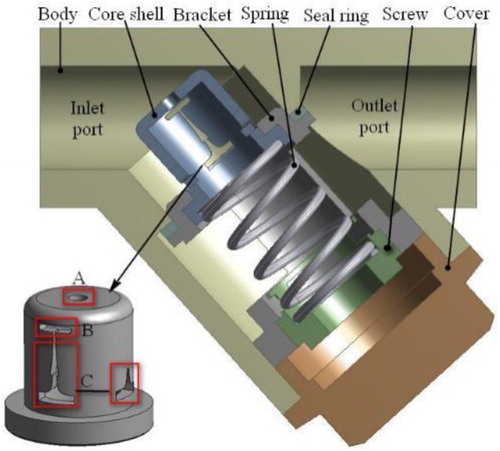
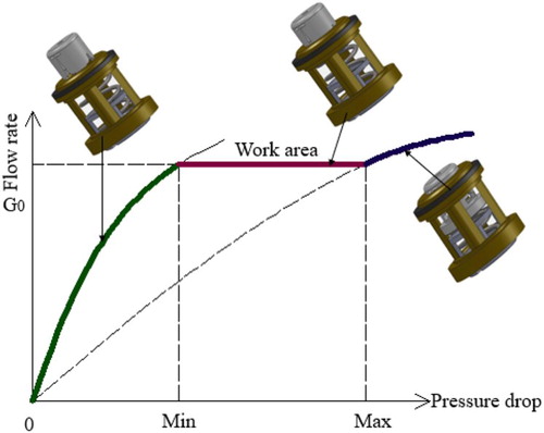
In order to describe in detail the operation of the dynamic balancing valve, Figure 2 shows three typical operating states of the balancing valve in the hydraulic system. When the balance valve pressure difference is lower than the minimum pressure difference, the ‘flow-pressure difference’ characteristic curve at this time is shown by the green line in Figure 2. The balance valve core stays in the initial position and the spring is not compressed. In this case, the flow rate is determined by the valve end face A, the side elliptical hole B and the variable opening C (Figure 1). The red line indicates the ‘flow-pressure difference’ characteristic curve of the balancing valve within the operating differential pressure range. As the pressure at the inlet increases, the hydraulic pressure acting on the spool gradually increases, moving the valve core in the ‘L2’ direction (Figure 4) length by interacting with the spring force, where the top of the short opening on the side is the starting point. In this case, the flow rate of the outlet is determined by the valve end face A, the side elliptical hole B and the variable section hole C. The purple line represents the ‘flow-pressure difference’ characteristic curve when the differential pressure of the balancing valve is greater than the maximum differential pressure. As the inlet pressure is further increased to the maximum pressure drop, the spring is fully compressed and the balancing spool moves to the maximum position. In this case, the flow rate of the outlet is determined by the valve end face A and the side elliptical hole B.

Figure 2. Operating status of dynamic flow balance valve in different pressure drops.

In the process just described, when the pressure changes, the valve core is moved by the coupling of the hydrodynamic force of the core face and the spring, and outlet port flow rate remains constant due to the change of the variable opening area of the valve core. Thus the core variable opening line is critical in the flow rate control process. Appropriate design of the orifice flow areas of the valve core can make the outlet port flow rate remain constant no matter how the inlet port pressure changes.

Design for the valve core

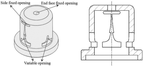
As is shown in Figure 3, the opening of the valve core is composed of the end face fixed opening, the side fixed openings, and the side variable opening, which uses asymmetrical hole structure to reduce valve core vibration caused by pressure pulsation.

Figure 3. Structure of dynamic flow balance valve core.

The position of the valve core is altered with pressure changes. The flow equation of the valve core can be written as (1) $Q=[C_1\times A_1+2C_i(A_i+A_2)]\sqrt{\frac{2\mathrm{\Delta }p}{\rho }},$(1) where Q is the flow rate of the balance valve, C₁ is the flow coefficient of the end face fixed opening, C_i is the flow coefficient of variable opening, A_i is the variable opening area under arbitrary displacement, A₁ is the area of the end face fixed opening, A₂ is the side face fixed opening area, Δp is the inlet and outlet port pressure drop, and ρ is the fluid density.

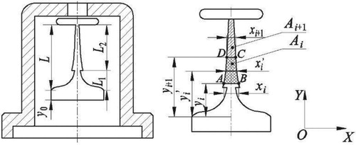
Figure 4 is a distribution model of the variable opening area of the valve core. The variable opening of the valve core along the Y direction is divided into N equal parts where $y_0=0,y_1,y_2,\dots ,y_i=(L/N)i,\dots ,y_N=L.$The corresponding x direction is $x_0,x_1,\dots ,x_i,\dots ,x_N,$where L is the core opening length and $i=1,2,\dots ,N-1.$When the valve is in operation, the valve core displacement is y_i. The spring compression is Y₀+y_i. The valve core flow area is A_i. The hydrodynamic force on the core face is balanced between with the linear spring force, therefore: (2) $\mathrm{\Delta }{p}_i=\frac{(Y_0+y_i)}{Y_0}\times \mathrm{\Delta }{p}_{min},$(2) where Δp_i is the pressure drop under an arbitrary displacement of the valve core. Y₀ is the initial compression of spring.

Figure 4. Variable opening area of valve core.

Using Equations (1) and (2), the variable opening area of core, A_i, can be obtained as follows: (3) $A_i=\frac{Q\sqrt{\frac{\rho Y_0}{2(Y_0+y_i)\mathrm{\Delta }{p}_{min}}-C\times A_1}}{2C_i}-A_2.$(3)

Using the principle of balance valve, the initial compression of the spring Y₀ can expressed as (4) $Y_0=\frac{p_1}{p_2-p_1}\times L.$(4)

When the valve reaches the operating state, then S_ABCD = A_i–A_i−1. It is assumed that the quadrilateral S_ABCD is approximately trapezoidal and can be expressed as (5) $S_{\text{ABCD}}=x_i^{\mathrm{\prime }}\times (y_{i+1}-y_i)=x_i^{\mathrm{\prime }}\times \frac{l}{n},$(5) (6) $x_i^{\mathrm{\prime }}=\frac{x_i+x_{i+1}}{2},$(6) (7) $x_i=\frac{x_i^{\mathrm{\prime }}+x_{i-1}^{\mathrm{\prime }}}{2}.$(7)

Using the above equations (5)–(7), x'_i and x_i can be calculated as (8) $x_i^{\mathrm{\prime }}=\frac{Qn}{2C_{i}L}\sqrt{\frac{\rho Y_0}{2\mathrm{\Delta }{p}_1}}\left[\sqrt{\frac{1}{Y_0+y_{i-1}}}-\sqrt{\frac{1}{Y_0+y_{i+1}}}\right],$(8) (9) $x_i=\frac{Qn}{4C_{i}L}\sqrt{\frac{\rho Y_0}{2\mathrm{\Delta }{p}_1}}\left[\sqrt{\frac{1}{Y_0+y_{i-1}}}-\sqrt{\frac{1}{Y_0+y_{i+1}}}\right].$(9) where i ∈ L. Then the calculation formula for the variable opening profile of the valve core can be derived using (10) $x_0=2\times x_0^{\mathrm{\prime }}-x_1{x}_n=2\times x_{n-1}^{\mathrm{\prime }}-x_{n-1}.$(10)

Methodology

To study the flow characteristics and flow rate control accuracy of the dynamic balance valve over its operating region, both computational analysis and experimental investigation were carried out (Ghalandari et al., 2019). These methods allow understanding of the flow characteristics within the valve internals and determination of the flow pattern. The hydrodynamic force error between the design and the simulation on the valve core face was analyzed using a computational tool. The methodology also allowed comparison of the results between the experimental and CFD method.

Experimental loop

The experimental facility used to investigate the flow balance valve was based on a closed water loop and is shown in Figure 5. The data acquisition control system measures the pressure drop and flow rate of the test valve under different working conditions by converting data from sensors into an electrical signal and is directly readable through special processing. The recirculating water system includes a water tank, a pump unit, a control valve, and a flow meter. By using a variable speed pump, the water from the water tank flows through the control valve A to the test valve, through control valve B and the flow meter, and then back to the water tank. In order to ensure the full development of turbulent flow before the test valve and the accuracy of flow and pressure tests, the flow meter is installed at a distance of 15 diameters from control valve A and the water tank. The pressure sensors are mounted before and after the test valve and the installation distance is five times the diameter of the pipe. Other installation locations are shown in Figure 5. The various parameters of the valve are shown in Table 1.

Figure 5. Experimental system for dynamic flow balance valve: (a) sketch map of the experimental system and (b) the test system of valve.

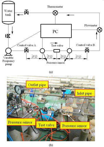
Table 1. Valve design parameters.

Parameters	Data
Diameter (mm)	15
Pressure drop (kPa)	15–150
Temperature (K)	298
Valve core displacement (mm)	11
Valve core outside diameter (mm)	17
Valve core inside diameter (mm)	13
Flow rate (m^3/h)	0.86

In this experimental system, the variable speed pump and the control valves A and B are used to supply the different water flow rates. The flow meter and pressure sensor are installed to measure the flow rate and the pressure drop of the test valve. The electromagnetic flow meter instrument accuracy level is 0.2%, and the pressure sensors instrument accuracy level is 1%. In order to obtain the system error and ensure the feasibility of the experiment, a probabilistic statistical method is used to calculate the errors of the system. It can be shown that (11) $\sigma =\pm \sqrt{\sum _{i=1}^n{\sigma }_i^2},$(11) where σ is the error of experimental system and σ_iis the error of each instrument.

According to this formula, the total system error is then ±1.42%. Since this value is within the allowable range of engineering error, the test measurement value is reliable.

Computational fluid dynamics modeling

Mathematical model

In general, the fluid herein is assumed to be an incompressible fluid. To analyze the flow characteristics inside the dynamic balance valve, the equations of the laws of conservation of mass, momentum, and energy were utilized by the software CFX to solve the principal of the fluid-flow correlated problems (Salih et al., 2019). At the same time, the outlet flux is calculated by the flow equation. The governing equations can be shown as follows: (12) $\text{div}(\rho v\varphi )=\text{div}({\mathrm{\Gamma }}_{\varphi }\text{grad}\varphi )+{\text{S}}_{\varphi }$(12) where ρ is the fluid density, ϕ refers to common variables (u, v, w, T), $\overrightarrow{v}$ is the velocity of medium, Γ_ϕ and S_ϕ are the generalized diffusion coefficients and source terms corresponding to ϕ.

In this study, the standard k-ϵ turbulent model was chosen (Zhou et al., 2018). It turns out that the standard k–ϵ is able to accurately describe the complex flow inside the valve (Hou et al., 2017; 2018; Iannetti et al., 2016). The turbulent kinetic energy k and the turbulent energy dissipation rate ϵ are expressed as (13) $\frac{(\mathrm{\partial }\rho k{u}_i)}{\mathrm{\partial }{x}_i}=\frac{\mathrm{\partial }}{\mathrm{\partial }{x}_j}\left[\left(\mu +\frac{{\mu }_t}{{\sigma }_k}\right)\frac{\mathrm{\partial }k}{\mathrm{\partial }{x}_j}\right]+P-\rho \epsilon ,$(13) (14) $\frac{(\mathrm{\partial }\rho \epsilon u_i)}{\mathrm{\partial }{x}_i}=\frac{\mathrm{\partial }}{\mathrm{\partial }{x}_j}\left[\left(\mu +\frac{{\mu }_t}{{\sigma }_z}\right)\frac{\mathrm{\partial }\epsilon }{\mathrm{\partial }{x}_j}+\frac{\epsilon }{k}(P{C}_{z1}-\rho C_{z2}\epsilon )\right],$(14) where u_i and x_i are respectively the velocity component and the co-ordinate in the direction i (i = 1, 2, or 3), t is the time, µ and u_t are the dynamic viscosity and the turbulent viscosity, and C_ϵ1, C_ϵ2, δ_k, and δ_ϵ are constants whose values are 1.44, 1.92, and 1.0, 1.3 respectively. The variable P is the turbulence production due to viscous forces, which is modeled using (15) $P={\mu }_t\left(\frac{\mathrm{\partial }{u}_i}{\mathrm{\partial }{x}_i}+\frac{\mathrm{\partial }{u}_j}{\mathrm{\partial }{x}_i}\right)\frac{\mathrm{\partial }{u}_i}{\mathrm{\partial }{x}_j},$(15) where µ_t is linked to the turbulence kinetic energy and dissipation via the relation in the k–ϵ model given by (16) ${\mu }_t=C_{\mu }\rho \frac{k^2}{\epsilon },$(16) where C_µ is a constant whose value is 0.09.

Boundary condition and grid

The medium in the dynamic balance valve is water, at a temperature of 298 K. Pressure inlets and outlets are the most commonly used boundary conditions. Different opening degrees are selected and the pressure difference before of the dynamic flow balance valve is calculated by formula (17). The outlet boundary condition is set to pressure outlet, and the pressure is set to 0 Pa. The pressure difference with different opening degrees is obtained as the pressure boundary condition. The pressure drop between the inlet and outlet for different displacement can be expressed as (17) $\begin{array}{rl}\mathrm{\Delta }{p}_i& =i\times (\mathrm{\Delta }{p}_{max}-\mathrm{\Delta }{p}_{min})/L+\mathrm{\Delta }{p}_{min},\\ & i=0,1,\dots ,11.\end{array}$(17)

Set the convergence conditions so that the maximum residual error is less than 1.0E–3, and the values of continuity, ramp speed, Y speed, Z speed, K and Epsilon are all less than 1.0E–4. The reference pressure is consistent with the actual working conditions and is set to 101.325 kPa. The three-dimensional flow channel model studied in this paper has a complex structure and requires high flow accuracy. This article uses a high-resolution format The remaining surfaces are set as no-slip walls.

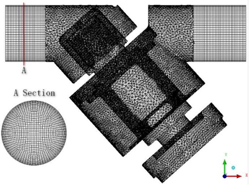
In order to achieve full development of the flow within the valve and exact outlet boundary conditions, the upstream and downstream pipework is included. Mesh quality and grid independence play important roles for the accuracy of the CFD result. Due to the complicated structure of the spool flow path, the method of automatically generating a grid is adopted. There is no fixed grid size similar to the simulation for the CFD method and the models need to be modified to allow a coarse mesh. Therefore, a grid independence check was tested before the numerical simulation (Xu et al., 2019). Changing the minimum edge and volume size to control the grid number of fluid zones, different mesh zones were built, which is shown in Figure 6. The variable y+ is used to describe the wall grid, and its value is related to the size of the wall boundary layer parameters and the Reynolds number. In this case, to ensure simulation accuracy, y⁺ near the wall region is required to be within 50 (Hou et al., 2017; Iannetti et al., 2016). By considering both calculation accuracy and resources, the grid number of the model is selected as 6.05e⁵, which is shown as Figure 7. For all other valve opening positions, model meshes were similar to the above.

Figure 6. Grid independence check.

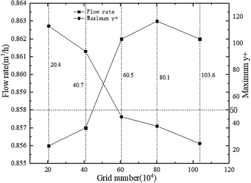
Figure 7. The grid of computational domain.

Optimization and performance and analysis of dynamic balance valve

Typical valve parameters are selected, and the specific parameters are shown in Table 1. According to the preliminary design method of the valve core opening line, the coordinates of each point were solved to fit the variable opening curve of the valve core using Visual Basic. The theoretical pressure drop of the valve core at different openings can be obtained by using Equation (18). This value is used as the boundary condition into the CFX software for the three-dimensional steady flow simulation. In this study, the SIMPLE procedure was adopted for velocity-pressure coupling (Li, Guo et al., 2017, Li, Wu et al., 2017; Qian, et al., 2019), and second-order upwind and central difference schemes were used to simulate convective and diffusion terms, respectively. The convergence criteria for continuity, velocity, and energy equations were set to 10⁻⁶.

Preliminary design structure calculation results

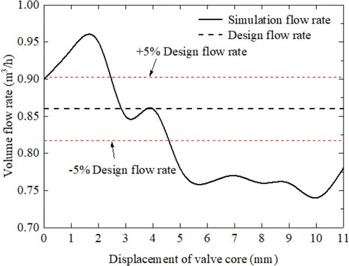
Figure 8 shows predicted flow rates at different openings. In the working pressure range, the flow rate is found to be out with the ±5% operation window of the desirable flow range of the design flow error line, For pressure drops at associated valve openings less than 3 mm the flow is predicted to be greater than 5%. Similarly, for pressure drops associated with valve positions greater than 6 mm, the flow is well outside the −5% limit, indicating a poorly performing valve.

Figure 8. Flow rate under different openings.

Valve core design optimization

In this part, the actual pressure which acts upstream and downstream of the valve core is monitored. The simulated pressure drop of the valve core can be obtained at different opening positions, and the error analysis is by comparison with the theoretical pressure drop. A comparison result of the test data is shown in Figure 9.

Figure 9. Comparison of theoretical and simulation of valve core pressure drop.

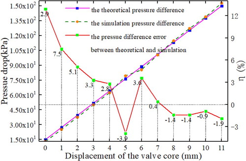
As seen in Figure 9, the theoretical and simulated pressure drops of the valve core are basically linearly increasing during the opening process, but there is an error between them. The maximum relative error at a core displacement of 0 mm and reaches 12.9%. The theoretical pressure drop is greater than the simulated pressure drop when the valve core displacement is between 0 and 4 mm, and the error value is gradually reduced. When the core displacement increases from 4 to 7 mm, the theoretical pressure is less than the simulated pressure drop, and when the valve core is between 7 and 11 mm, the error slowly increases, and finally stays within −2% or less. As can be seen from Figure 9, the pressure difference error between theoretical and simulation is a gradual downward trend. However, when the pressure drop at a displacement of 5 mm drops sharply, the valve core is located at the junction of the longer variable opening and the shorter variable opening on the side, resulting in a sharp drop in pressure drop.

According to the data results in Figure 9, a pressure compensation coefficient factor, ϵ_i, can be constructed. Using the least squares polynomial fitting method to find the curve of the error data and solving the corresponding functional relation yields the pressure drop compensation coefficient factor and the correction function of the dynamic flow balance valve. It can be written as

(18) $\begin{array}{r}{\epsilon }_i=\{\begin{array}{l}0.13i^4-1.18i^3+4.12i^2-4.48i+12.90\begin{array}{r}\end{array}(0\le i<4)\\ 8.58e-39e^{3.55i}\begin{array}{ccc}\begin{array}{ccc}\begin{array}{ccc}& & \end{array}& & \end{array}& & \end{array}\begin{array}{r}\end{array}(4\le i<8)\\ -0.03i^4+0.90i^3-8.21i^2+24.66i+35\begin{array}{r}\end{array}(9\le i<11),\end{array}\end{array}$(18) where i is the core displacement.

The pressure drop p′_, which has been revised under any opening may be obtained by substituting the compensation coefficient factor correction function into Equation (19). (19) $p_i^{\mathrm{\prime }}=\frac{Y_0+y_i}{Y_0}\times p_1\times {\epsilon }_i.$(19)

Then Equations (8) and (9) give the deformation as (20) $\begin{array}{rl}\underset{i}{\overset{\bullet }{x}}& =\frac{Qn}{2C_{i}L}\sqrt{\frac{\rho Y_0}{2\mathrm{\Delta }{p}_1}}[\sqrt{\frac{1}{(Y_0+y_i){\epsilon }_i}}\\ & -\sqrt{\frac{1}{(Y_0+y_{i+1}){\epsilon }_{i+1}}}],\end{array}$(20) (21) $\begin{array}{rl}\stackrel{\bullet }{x}& =\frac{Qn}{4C_{i}L}\sqrt{\frac{\rho Y_0}{2\mathrm{\Delta }{p}_1}}[\sqrt{\frac{1}{(Y_0+y_{i+1}){\epsilon }_{i-1}}}\\ & -\sqrt{\frac{1}{(Y_0+y_{i+1}){\epsilon }_{i+1}}}],\end{array}$(21) where i ∈ L. The revised core profile calculation formula of the variable opening is then (22) $\underset{0}{\overset{\bullet }{x}}=2\times x_0^{\mathrm{\prime }}-\underset{1}{\overset{\bullet }{x}},$(22) (23) $\underset{n}{\overset{\bullet }{x}}=2\times x_{n-1}^{\mathrm{\prime }}-\underset{n-1}{\overset{\bullet }{x}}.$(23)

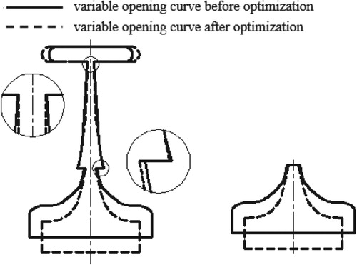
The revised formula was used with Visual Basic to compile the procedures to solve for the coordinates of each point, fitting the core variable opening curve as shown in Figures 10 and 11.

Figure 10. Variable opening curve of the valve core before and after optimization.

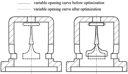
Figure 11. Enlarged image of the variable opening profile of the core before and after optimization.

Results and discussion

CFD simulation comparative analysis

The simulated flow rate curve of the core before and after optimization is shown in Figure 12. It can be found that the flow rate before optimization is basically more than ±5% of the standard flow error line in the entire working pressure range. When the displacement of the valve core is less than 1 mm, the simulated flow is more than +5% of the standard flow error line, and when the displacement is more than 2 mm, the simulated flow is less than –5% of the standard flow error line. In this case, the hydraulic imbalance is serious. The flow rate after optimization is within the acceptable bounds of the standard flow rate, mainly concentrated close to the −5% standard flow error line.

Figure 12. Comparison of simulation flow curve before and after optimization.

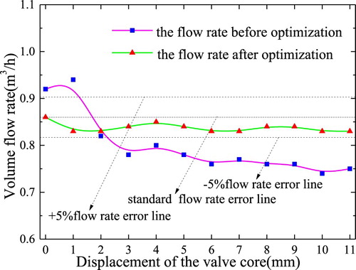
Figure 13 shows the comparative analysis results of the CFD simulation flow error before and after optimization. It can be seen that when the displacement of the valve core is less than 2 mm or more than 9 mm, the simulated flow curve before optimization exceeds the flow accuracy tolerance, and the maximum error reaches 18.2%. The accuracy of the optimized flow is within the acceptable range of error, and the average error is about 2.3%, which complies with the requirements of valve flow rate control accuracy.

Figure 13. Comparison of simulation flow rate error curve before and after optimization.

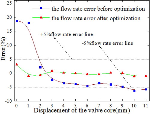
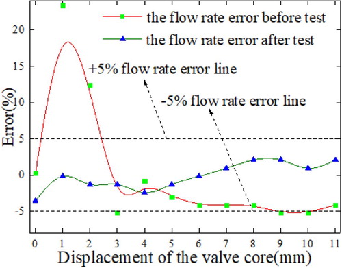
Figure 14 shows the comparison between the results of the flow rate obtained from the CFD simulation and experiments performed before and after optimization of the valve core. It can be seen that the simulation and test flow variation trend is consistent before optimization, they both first increase and then decrease and finally become relatively consistent. The flow fluctuation is serious when the displacement of the core is between 0 and 3 mm. The flow rate obtained by simulation and test is in a smooth transition after optimization with consistent change trends. In Figure 14, the trends of the test and simulation curves show good agreement. Machining errors and differential pressure measurement errors are the main causes of errors between test values and numerical simulation values. Besides, the CFD software has limited accuracy when performing numerical simulations, and there must be a certain deviation in calculation and test results. The trend of the test curve and the simulation curve is generally consistent, which confirms the correctness of the simulation. Figure 15 shows the comparison between the results of the flow accuracy errors obtained from the experiments before and after optimization of the valve core. The flow accuracy error exceeds the +5% flow accuracy error limit when the displacement of core is between 0.5 and 2.5 mm before optimization and the maximum error reaches 17.2%. In addition, it slightly exceeds the −5% flow accuracy error limit when the displacement of the core is between 9 and 10 mm. The flow accuracy error is within the error limit after optimization since the average error is about 3.4%, which complies with the requirements of valve flow rate control accuracy.

Figure 14. Comparison of the test and simulation flow rate before and after optimization.

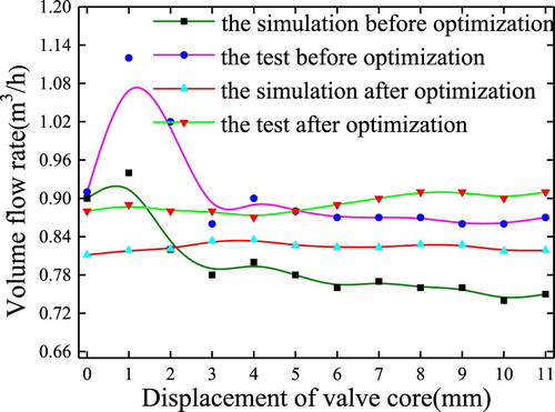
Figure 15. Comparison of the test flow rate error before and after optimization.

The effect of key parameters on flow accuracy

The dynamic flow balance valve enables a constant output flow rate during the operation process by changing the valve core displacement. Valve core displacement is achieved by coupling the spring force and fluid dynamic force acting on the valve core. However, there are some errors between the actual selection of spring stiffness and the theoretical calculation of spring stiffness caused by factors such as machining burrs on the core surface in the actual production process and the shell design both of which affect the flow accuracy of the balance valve. Therefore, it is essential to study the effects of key factors such as spring stiffness, burr, and core-shell geometry design. In this section, the experimental system of the dynamic flow balance valve was used to analyze the impact of these factors.

The effect of different spring stiffness

According to the theoretical calculated spring stiffness, three groups of spring stiffness were selected and analyzed. Figure 16 shows the effective behavior of the balance valve flow rate in the three groups when other structural parameters are unchanged.

Figure 16. Flow rate curves of balance valve under different spring stiffness.

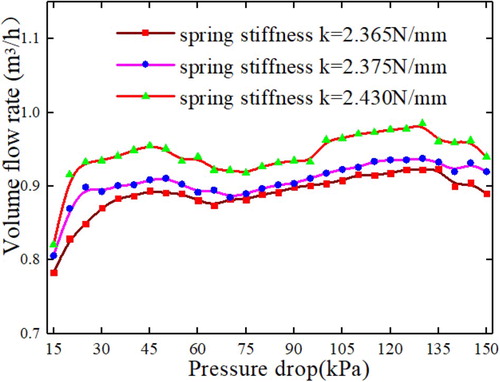
As seen in Figure 16, the flow rate of the different spring stiffnesses in the balance valve is approximately the same. When the pressure drop is changed, the flow rate increases with the increase in spring stiffness. With the same pressure drop, the flow value is different under different spring stiffness. Under the same conditions, the greater the spring stiffness, the smaller the value core displacement, the greater the opening of the valve, and the larger the flow value.

The effect of different core shell structure

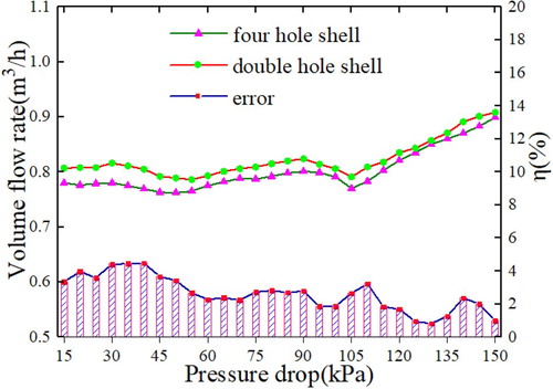
As is shown in Figure 17, the shell design of the balance valve core is a double-hole shell initially. Taking into account the requirements of the internal flow stability of the balance valve. A four-hole design was manufactured and investigated. The effects on the balance valve flow with different core-shell designs were analyzed comparatively with other parameters unchanged. The comparison result of the outlet flow rate of the balance valve with different valve core-shell design is shown in Figure 18. The change of core-shell design will have an influence on the flow rate, and the variation trends of the two structures are consistent. The flow magnitude of the balance valve under the four-hole shell structure valve is larger than that of the double-hole shell structure. The maximum difference between the two is 4.4%, and the average difference is about 2.6%. Where the maximum difference of 4.4% refers to the maximum difference value between the flow value of the four-hole shell structure and the flow value of the double-hole shell structure of different pressure difference. The valve core displacement changes as the pressure drop changes. Under different pressure drops, the relative position of the valve core and the housing structure changes, which makes the flow value different under different housing structures.

Figure 17. (a) Bracket 2D view, (b) Bracket prototype.

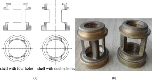
Figure 18. Comparison of the flow rate under different valve core-shell structure.

The effect of the valve core burrs

Machining burrs always exist on the surface of a valve core and result from the specific production process, and due to the small orifice flow areas may have an impact on the flow of the balance valve. By carrying out a flow test with burrs in place the effect on the balance valve can be determined. The compared result for the two conditions is shown in Figure 19.

Figure 19. Comparison of the flow rate under different machining precision.

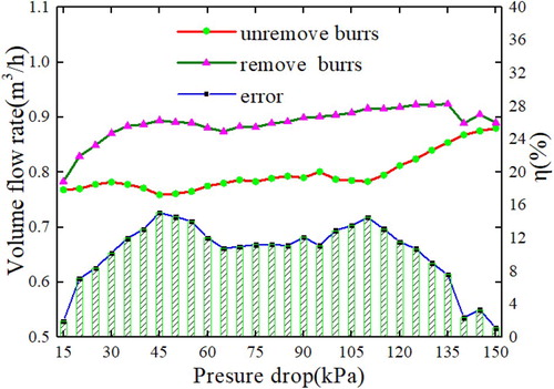
As seen in Figure 19, the surface roughness of the valve core assembly will have an influence on the flow value of the dynamic flow balance valve. The flow value after finishing of the valve core assembly is greater than the flow rate of the original structure. At the minimum differential pressure and the maximum differential pressure positions, these flow values are relatively close to each other. At other differential pressure locations, the flow values of the two are quite different, with a maximum difference of approximately 14.2%. Where the maximum different value of 14.2% refers to the difference between the flow value when the burr is removed and the flow value when the burr is not removed under the different pressure difference. The average difference value is approximately 10.1% during the entire flow adjustment process. The valve core displacement changes with pressure drop. Under different pressure drops, the contact area between the valve core and the fluid changes, resulting in different surfaces and different flow values of the valve.

Conclusion

The study investigated the optimization of the valve core structure by the pressure drop compensation coefficient revising method, and the effect of different key parameters on the flow rate control accuracy was discussed. The experimental and numerical simulations were carried out on a dynamic balance valve under different operating conditions. The numerical simulation results agree well with the experimental results in different pressure drops. The test results verify the effectiveness of the optimization method and the applicability of the CFD numerical simulation method. The following conclusions were obtained.

It has been possible to improve the accuracy of flow control by implementing a pressure drop compensation coefficient revising method to optimize the balance valve core. Through the revision of the variable opening profile of the core, the flow control accuracy meets the ±5% error requirements.

The spring stiffness has an effect on the flow rate of the dynamic flow balance valve. The flow rate increases corresponding to the increase of the spring stiffness.

The change of the core-shell structure will affect the flow rate of the dynamic flow balance valve. The flow rate of the balance valve under the four-hole shell structure is larger than that of double holes shell structure, and the average error between the two designs is about 2.6%.

The existence of machining burrs on the surface of the valve core has an influence on the flow rate of the dynamic flow balance valve. The flow rate after removing the burrs is greater, and the average error between them is about 10.1%.

In short, whether to remove the burr has a greater impact on the flow value accuracy, while the impact of spring stiffness and the core shell structure is relatively small. These results provide the theoretical support for improving the accuracy of flow control and provide a reference for the future design of dynamic flow balance valve. In the future, it is recommended to carry out vibration analysis and research on the valve core of the dynamic flow balancing valve to further improve the stability of the valve core.

Notation

ρ	=	density (kg/m3)
SABCD	=	the area of micro unit (mm2)
Q	=	total flow (m3 /h)
xi'	=	the midline between xi and xi+1 (mm)
L	=	total displacement of valve spool (mm)
yi'	=	the midline between yi and yi+1 (mm)
p2	=	the maximum working pressure difference (kPa)
mspool	=	valve spool quality (kg)
p1	=	the minimum working pressure difference (kPa)
Fspring	=	spring force (N)
C1	=	flow coefficient of end face fixed opening (–)
K	=	spring stiffness (N/mm)
Ci	=	flow coefficient of variable opening (–)
F0	=	pre-tightening force by spring (N)
A1	=	end face fixed opening area (mm2)
$\ddot{x}$	=	valve spool acceleration (m/s2)
A2	=	side face fixed opening area (mm2)
Fwater	=	the medium force upon on the end surface (N)
pi	=	working pressure difference under arbitrary displacement (kPa)
Fflow	=	the medium force upon on the side surface (N)
Y0	=	the initial amount of compression of spring (mm)
FN	=	the medium force inside on the side surface (N)
Ai	=	variable opening area under arbitrary displacement (mm2)
Ff	=	friction force between valve spool and valve shell (N)
yi	=	arbitrary displacement along the axial direction of valve spool (mm)
pi'	=	the pressure under arbitrary displacement after revision (kPa)
xi	=	projection under arbitrary displacement along the X direction (mm)
ϵi	=	differential pressure compensation coefficient factor (–)
$\dot{x}$i	=	projection after revision under arbitrary displacement along the X direction (mm)
$\dot{x}$i′	=	the midline after revision between xi and xi+1 (mm)
$\eta$	=	the deviation between the two (%)

Acknowledgments

The authors would like to thank the National Natural Science Foundation of China (grant number 51569012) for the financial support.

Disclosure statement

No potential conflict of interest was reported by the author(s).

Additional information

Funding

This work was supported by the National Natural Science Foundation of China: [Grant Number No. 51569012].

References

- Akbarian, E., Najafi, B., Jafari, M., Ardabili, S. F., Shamshirband, S., & Chau, K. W. (2018). Experimental and computational fluid dynamics-based numerical simulation of using natural gas in a dual-fueled diesel engine. Engineering Applications of Computational Fluid Mechanics, 12(1), 517–534. https://doi.org/10.1080/19942060.2018.1472670
- Aung, N. Z., Yang, Q., Chen, M., & Li, S. J. (2014). CFD analysis of flow forces and energy loss characteristics in a flapper-nozzle pilot valve with different null clearances. Energy Conversion and Management, 83, 284–295. https://doi.org/10.1016/j.enconman.2014.03.076
- Cui, B., Lin, Z., Zhu, Z., Wang, H. J., & Ma, G. F. (2017). Influence of opening and closing process of ball valve on external performance and internal flow characteristics. Experimental Thermal & Fluid Science, 80, 193–202. https://doi.org/10.1016/j.expthermflusci.2016.08.022
- Ghalandari, M., Bornassi, S., Shamshirband, S., Mosavi, A., & Chau, K. W. (2019). Investigation of submerged structures’ flexibility on sloshing frequency using a boundary element method and finite element analysis. Engineering Applications of Computational Fluid Mechanics, 13, 519–528. https://doi.org/10.1080/19942060.2019.1619197
- Hou, C. W., Qian, J. Y., Chen, F. Q., Jiang, W. K., & Jin, Z. J. (2017). Parametric analysis on throttling components of high multi-stage pressure reducing valve. Applied Thermal Engineering, 128, 1238–1248. https://doi.org/10.1016/j.applthermaleng.2017.09.081.
- Huovinen, M., Kolehmainen, J., Koponen, P., Nissilä, T., & Saarenrinne, P. (2015). Experimental and numerical study of a choke valve in a turbulent flow. Flow Meas & Instrum, 45, 151–156. http://doi.org/10.1016/j.flowmeasinst.2015.06.005
- Iannetti, A., Matthew, T., Stickland, X., & William, M. D. (2016). A CFD and experimental study on cavitation in positive displacement pumps: Benefits and drawbacks of the ‘full’ cavitation model. Engineering Applications of Computational Fluid Mechanics, 10, 57–71. https://doi.org/10.1080/19942060.2015.1110535
- Li, B., Guo, S., Mao, X. Y., Wu, C., Zhang, D. M., Shang, J., & Liu, Y. S. (2017). Characteristic analysis and experiment of a dynamic flow balance valve. Earth and Environmental Science, 100, 012107. https://doi.org/10.1088/1755-1315/100/1/012107
- Li, S. Y., Wu, P., Cao, L. L., Wu, D. Z., & She, Y. T. (2017). CFD simulation of dynamic characteristics of a solenoid valve for exhaust gas turbocharger system. Applied Thermal Engineering, 110, 213–222. https://doi.org/10.1016/j.applthermaleng.2016.08.155
- Liu, J. B., Xie, H. B., Hu, L., Yang, H. Y., & Fu, X. (2017). Realization of direct flow control with load pressure compensation on a load control valve applied in overrunning load hydraulic systems. Flow Measurement and Instrumentation, 53, 261–268. http://doi.org/10.1016/j.flowmeasinst.2016.07.004
- Pietrzak, M., & Witczak, S. (2015). Experimental study of air-oil-water flow in a balancing valve. Journal of Petroleum Science & Engineering, 133, 12–17. https://doi.org/10.1016/j.petrol.2015.05.019
- Qian, J. Y., Wei, L., Jin, Z. J., Wang, J. K., Zhang, H., & Lu, A. L. (2014). CFD analysis on the dynamic flow characteristics of the pilot-control globe valve. Energy Conversion and Management, 87, 220–226. https://doi.org/10.1016/j.enconman.2014.07.018
- Qian, J. Y., Wu, J. Y., Gao, Z. X., Wu, A. J., & Jin, Z. J. (2019). Hydrogen decompression analysis by multi-stage Tesla valves for hydrogen fuel cell. International Journal of Hydrogen Energy, 44(26), 13666–13674. https://doi.org/10.1016/j.ijhydene.2019.03.235
- Ramanath, H. S., & Chua, C. K. (2006). Application of rapid prototyping and computational fluid dynamics in the development of water flow regulating valves. International Journal of Advanced Manufacturing Technology, 30(9–10), 828–835. https://doi.org/10.1007/s00170-005-0119-5
- Ryu, S. R., Rhee, K. N., Yeo, M. S., & Kim, K. W. (2008). Strategies for flow rate balancing in radiant floor heating systems. Building Research & Information, 36(6), 625–637. https://doi.org/10.1080/09613210802450697
- Salih, S. Q., Aldlemy, M. S., Rasani, M. R., Ariffin, A. K., Ya, T. M. Y. S. T., Al-Ansari, N., Yaseen, Z. M., & Chau, K. W. (2019). Thin and sharp edges bodies-fluid interaction simulation using cut-cell immersed boundary method. Engineering Applications of Computational Fluid Mechanics, 13, 860–877. https://doi.org/10.1080/19942060.2019.1652209
- Shen, X. R., Lu, B., Li, J. L., & Li, Z. Z. (2006). The numerical analysis and experimental investigation of automatic flux compensation valve. Chinese Pneumatics & Seals, 1, 56–58.
- Taylor, S. T., & Stein, J. (2002). Balancing variable flow hydronic systems. Ashrae Meeting, 4, 17–25.
- Wu, D., Li, S., & Wu, P. (2015). CFD simulation of flow-pressure characteristics of a pressure control valve for automotive fuel supply system. Energy Conversion & Management, 101, 658–665. https://doi.org/10.1016/j.enconman.2015.06.025
- Xu, X. G., Liu, T. Y., Li, C., Zhu, L., & Li, S. X. (2019). A numerical analysis of pressure pulsation characteristics induced by unsteady blood flow in a bileaflet mechanical heart valve. Processes, 7(4), 232. https://doi.org/10.3390/pr7040232
- Zhou, L., Bai, L., Li, W., Shi, W. D., & C, W. (2018). PIV validation of different turbulence models used for numerical simulation of a centrifugal pump diffuser. Engineering Computations, 35(1), 2–17. https://doi.org/10.1108/EC-07-2016-0251