Integral pumping rings for dual mechanical seals: hydraulic performance evaluation using numerical simulations

ABSTRACT

The flow of barrier fluid through an industrial pressurized dual mechanical seal cartridge is investigated and evaluated experimentally and numerically. The cartridge is of the bi-directional type wherein it is radial-flow designed and fitted with a bi-directional integral pumping ring. The standard k–ϵ turbulence model is applied and the multiple frame of reference method is utilized to simulate the motion of the pumping ring. The present study is a continuation of former experimental and numerical companion work conducted in the area of the design and evaluation of integral pumping rings for dual mechanical seals. In the present study, barrier fluid flow is visualized to provide internal insight of the flow behavior leading to a better understanding of the pumping mechanism on both quantitative and qualitative aspects. The flow field is evaluated and a number of design defects are revealed. The simulations show that barrier fluid is being trapped in closed circulation in the inboard-seal region, consequently implying weaker regeneration of barrier fluid in that region in comparison with the outboard-seal region. Moreover, the simulations also reveal the existence of a relatively large separation zone at the outlet port leading to increased losses and reduced flow rate capacity of the device.

Keywords:

• Dual mechanical seals
• integral pumping rings
• barrier fluid
• flow visualization

1. Introduction

In a typical conventional mechanical seal setup, a single seal is used which entails a stationary and a rotating ring. In this case, the process fluid provides the lubricating film between the seal's rubbing faces. If the seal is working properly, the lubricating fluid leaks in a predetermined amount to the other side of the seal; typically, the atmospheric ambient. This leak takes place in the form of minute droplets or vapor relying on a number of operating conditions such as the seal design, fluid type and working temperature. However, in some situations the process fluid cannot be used for this purpose and, therefore, the conventional seal setup becomes an impractical choice. Volatile compounds and toxic and air pollutant fluids are instances of such process fluids where the conventional seal setup should not be used to reduce the adverse environmental footprint and to meet regulatory legislation. Another example is when the process fluid lacks proper lubrication properties, such as crystallizing, state-changing and gaseous fluids. Moreover, even if the process fluid is of good lubricity and environmentally friendly, the conventional setup might still be an impractical choice in applications requiring back-up seals—such as when expensive process fluids are used or machines are critical to a plant (Blaber, 2003).

As a substitute to the conventional setup, the double mechanical seal is introduced to tackle the aforementioned limitations. As shown in Figure 1, a double mechanical seal cartridge entails: (1) an inboard seal, (2) an outboard seal and (3) a barrier fluid in between. The inboard seal separates the process and barrier fluids while the outboard seal isolates the latter from the atmospheric ambient. In the present context, the barrier fluid is different in nature from the process fluid and is pressurized to provide the lubricating films for both seals. Therefore, the barrier fluid circulates in a dedicated piping loop, passing through a variety of components to regulate and monitor its flow such as filters, valves and coolers. Typically (API, 2012), the barrier fluid is circulated in its piping system using one of the following three methods. The first method is to implement natural thermal convection where the temperature of the barrier fluid outflow from the cartridge is higher than that of the cooled inflow. The second method is to implement an integral pumping ring, which is a pumping ring installed on the machine's shaft between the two seals within the cartridge, as shown in Figure 1. Finally, the last alternative is to use an external pumping device for the barrier fluid loop.

However, the present study is concerned with the second pumping method, since it is the most common method in industrial setups owing to its practicality compared with the other methods (Smith, 2010). This is because elevated operation temperatures and lower specific flow rates undermine the thermal convection method compared with the integral pumping rings. Moreover, using a dedicated external pumping device and its conjugate auxiliaries for the barrier fluid loop is more expensive and bulky compared with the (relatively) compact design of dual seals with integral pumping rings. For a more detailed review of available standard seal setups, the reader is referred to API (2012), Smith (2014) and Forsthoffer (2017).

Experimental tests have been conducted by Carmody et al. (2007) comparing the flow-head curves of different designs of pumping rings. Also, numerical visualization of flow through internal cavities of a typical seal was conducted for flow path optimization. Moreover, the inspiring work of Luan and Khonsari (2006, 2007) is worth highlighting here, even though their work addresses a classical seal setup. This is because it was illustrated how the flow patterns of flushing fluids in the vicinity of the sealing surfaces can be interpreted to evaluate the effectiveness of cooling performance. It is noted, however, that limited published literature is available about the performance evaluation of integral pumping rings for dual seal cartridges, even though this design has been widely applied in the industry. For this reason, the previous companion works (Warda et al., 2016, 2018a, 2018b; Warda, Wahba, et al., 2018; Warda et al., 2015) and the present one have been conducted in a quest to enrich the available literature investigating various designs of integral pumping rings for dual mechanical seals. In the first companion work (Warda et al., 2015), experimental and numerical setups were constructed to review the hydraulic performance of axial and radial flow integral pumping rings, which was the foundation stone of the following studies. After that, in Warda et al. (2016), the influence of barrier fluid properties on the hydraulic performance of radial flow pumping rings was investigated experimentally. Moreover, the study was further extended in Warda et al. (2018b) to treat the remaining designs of axial-flow type. Additionally, generalized empirical correlations were proposed based on the experimental observations replacing the conventional $Q-\mathrm{\Delta }P$ curves by generalized ${\pi }_1-{\pi }_2$ characteristic curves. While on the numerical aspect, a detailed numerical parametric study was conducted by Warda et al. (2018a) to enhance the previous numerical model of Warda et al. (2015). Moreover, the numerical domain size was extended to treat the inboard sealing surfaces. Finally, a detailed numerical analysis was conducted by Warda, Wahba, et al. (2018) visualizing barrier fluid flow through an axial flow pumping ring – the axial pumping scroll.

Numerical simulations of barrier fluid flow through dual mechanical seals are challenging for a number of reasons. First, the fluid domain is characterized by being highly non-amenable due to tight clearances and multiple intersections of different geometries, consequently posing a considerable toll on obtaining a quality computational grid. Moreover, such a geometry also gives rise to serious flow instabilities and induces secondary flows such as separations and stagnation points. Furthermore, the flow field is highly inertial, specially at elevated operational speeds and temperatures leading to highly turbulent and intense swirling flows. In the present study, the previous enhanced numerical model of Warda et al. (2018a) is used to provide detailed internal insights of the barrier fluid flow through a commercial dual seal cartridge of the MPW-RO-RI type, shown in Figure 2. The cartridge is of the radial flow type and is characterized by the following three main attributes: a modified paddle wheel (MPW) bi-directional pumping ring; a radial-inlet (RI) port; and a radial-outlet (RO) port. A major characteristic of this design is its independence of direction of rotation and hence the name ‘bi-directional’. Moreover, despite being hydrodynamically inferior to most scroll-type pumping rings (see for example Figure 3) (Bloch, 2017b; Warda et al., 2018b), the MPW design considered in the present study is superior in industrial applications where shaft deflection is anticipated (Bloch, 2017b). This is because the axial-flow family in general relies on tight clearance between the ring and its housing, while, on the other hand, radial-flow types rings can operate with more permissive clearance, as will be illustrated in what follows.

Figure 1. A simplified schematic diagram for a pumping-ring dual-mechanical-seal cartridge.

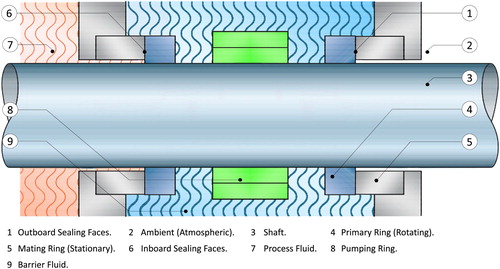
Figure 2. Experimental setup photographs for: (a) an MPW pumping ring; (b) an installed MPW pumping ring; (c) a fully assembled sealing cartridge; and (d) a cartridge installed on the pumping train.

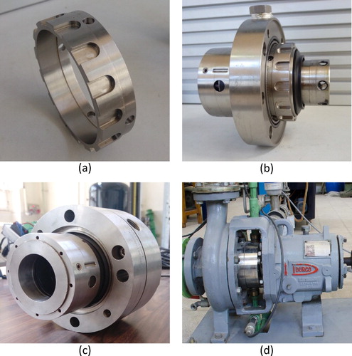
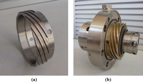
Figure 3. Photographs of (a) a pumping scroll and (b) a pumping scroll installed in a seal cartridge.

2. Experimental setup

An experimental setup is constructed complying with the schematic shown in Figure 4. The setup mainly entails the process fluid and the barrier fluid loops, illustrated by subfigures (a) and (b) in Figure 4 respectively. In the process fluid loop, the fluid stored in a pressurized tank (1) is pumped through the loop by means of a centrifugal pump (2) back to the tank, forming a recirculation system. The pump is driven by a 3.5 kW AC induction motor controlled by a frequency inverter to vary its rotational speed. The pressure and temperature of inlet and outlet process fluid to the pump are monitored by means of pressure (3) and temperature (4) transmitters, respectively. The pressurized tank pressure is controlled, if needed, by means of injecting/venting pressurized air through a ball valve (5). Finally, the pump flow rate is controlled by means of a gate valve (6).

Figure 4. Schematic diagrams for the process (a) and barrier (b) fluid loops (Warda et al., 2018a).

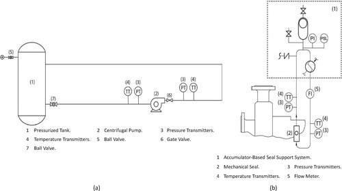
On the other hand, the barrier fluid loop is constructed in compliance with the ‘53B’ piping plan of the API-682 standard (API, 2012). As shown in Figure 4, the fluid is supplied from the accumulator-based seal support system (1) where the loop's pressure is controlled by a bladder type accumulator and the temperature is regulated by means of a heat exchanger. The fluid is circulated through the loop by means an integral pumping ring within the mechanical seal cartridge (2). The inlet and outlet barrier fluid's pressure and temperature to the cartridge are monitored by means of the pressure (3) and temperature (4) transmitters, respectively. Moreover, the mass flow rate is monitored by a Coriolis flow meter (5).

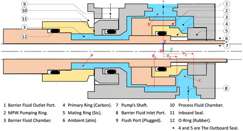
The installed mechanical seal cartridge is a pressurized commercial cartridge (John Crane cartridge T.3648) as shown in Figure 2, which is classed as a ‘face-to-back’ dual seal of ‘Arrangement 3’ in accordance with API-682 standard conventions (API, 2012). Figure 5 shows a simplified cross-sectional view of the tested cartridge design. The cartridge is fitted with an MPW pumping ring having both barrier inlet and outlet ports oriented radially. It is hence referred to as an MPW-RO-RI cartridge.

Figure 5. A simplified cross-sectional view of the MPW-RI-RO dual seal cartridge. The simulated barrier fluid domain is highlighted in blue.

In the present study, the $Q-\mathrm{\Delta }P$ performance curve of the MPW-RI-RO cartridge was obtained with water as the working barrier fluid at a speed of 3600 rpm. First, the pump operation speed was maintained at the desired value by means of an AC frequency inverter. Second, once steady operation conditions were observed, the inlet and outlet pressure and flow rate of the barrier fluid loop were measured; therefore, a single operation point was indicated. Lastly, the barrier flow rate was varied by means of a flow control valve in the loop to obtain the next operation point, following the same procedure. Table 1 illustrates the uncertainty values of the measuring instrumentation implemented, as calibrated by their corresponding vendors.

Table 1. Accuracy values of the various instrumentation in the experimental setup.

Instrument	Resolution
PT	$0.1\mathrm{\%}$ of span
TT	$0.2\mathrm{\%}$ of span
MFM	$\pm 0.15\mathrm{\%}$ of measurement
SFI	0.01 Hz

3. Numerical model

A numerical model is constructed using the commercial computational fluid dynamics (CFD) package ANSYS FLUENT^®. Domain decomposition, discretization, numerical methods, governing equations, numerical validation and verification are illustrated in what follows.

3.1. Domain geometry and mesh generation

Figure 5 presents a cross-sectional view of the simulated dual seal cartridge, wherein the numerical domain of the present study examines the fluid zone highlighted in blue. Compared with the previous companion model (Warda et al., 2015), the present model treats the region of the inboard-seal and, therefore, the whole barrier fluid domain is simulated in the present study without omission. Figure 6 shows the three-dimensional extracted barrier fluid volume to be simulated, i.e. the geometry of the simulated fluid domain. The domain occupies a 105.5 mm × 79.422 mm × 294.31 mm bounding box in the x-, y- and z-directions, respectively. Moreover, the modeled fluid domain occupies a volume of 1.5065 × 10${}^5$ mm${}^3$.

Figure 6. Computational domain of the barrier fluid.

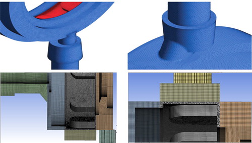
The discretization of the fluid domain considered in the present work is a major innovation. This is because one can see from the cross-sectional view of Figure 5 that the do is not amenable. In other words, it is characterized by sudden changes of volume and various types and orientations of intersecting geometry. This, in turn, leads to two main choices when discretizing the domain. The first, and the easiest, choice is to use a tetrahedral mesh, which was used in the previous companion model (Warda et al., 2015). Owing to the unstructured nature of tetrahedral-type grids, such a complicated domain can be discretized at once. However, the major disadvantage here is the increased numerical diffusion due to the crude non-orthogonality of the cell faces and the flow flux. Moreover, cells are seeded and populate the numerical domain without compliance with the flow direction. On the other hand, the second discretization of choice is to implement structured high-quality elements, such as hexahedrons or prisms, with the cells oriented as much as possible with the overall flow direction. However, the major limitation here is the complexity of the simulated domain to be filled in such a structured manner. For this reason, the numerical domain in the present study is decomposed into a number of sub-domains where each sub-domain is meshed independently of the other zones; therefore, a multi-zone mesh is created. The domain is decomposed in such a way that most of the resulting sub-domains are amenable and, therefore, can be structured-meshed. However, the remaining non-amenable zones are meshed tetrahedrally, resulting in an overall hybrid computational domain as shown in Figure 7.

Figure 7. Illustration of the tetrahedral grid implemented in Warda et al. (2015) (top) versus the hybrid-grid multi-zone grid in the present work and in Warda et al. (2018a) (bottom).

3.2. Transport equations and boundary conditions

In the present study, the Reynolds-averaged Navier–Stokes transport equations were used in three-dimensional Cartesian coordinates. The barrier fluid flow was assumed to be steady, incompressible and isothermal: (1) $\begin{array}{rl}\frac{\mathrm{\partial }{u}_i}{\mathrm{\partial }{x}_i}=& 0\end{array}$(1) (2) $\begin{array}{rl}\frac{\mathrm{\partial }\left(u_i{u}_j\right)}{\mathrm{\partial }{x}_j}=& -\frac{1}{\rho }\frac{\mathrm{\partial }P}{\mathrm{\partial }{x}_i}+\frac{1}{\rho }\frac{\mathrm{\partial }}{\mathrm{\partial }{x}_i}[\mu (\frac{\mathrm{\partial }{u}_i}{\mathrm{\partial }{x}_j}+\frac{\mathrm{\partial }{u}_j}{\mathrm{\partial }{x}_i})]\\ & +\frac{1}{\rho }\frac{\mathrm{\partial }{\tau }_{\mathrm{t}\mathrm{u}\mathrm{r}\mathrm{b}}}{\mathrm{\partial }{x}_i},\end{array}$(2) where $u_i$ are the velocity field components, P is the pressure, ρ is the fluid density, μ is the dynamic viscosity and ${\tau }_{\mathrm{t}\mathrm{u}\mathrm{r}\mathrm{b}}$ is the turbulence stress tensor. The two-equation eddy viscosity based model k–ϵ (Launder & Spalding, 1983) is used to model turbulence. The model entails two transport equations: the first one is the turbulent kinetic energy (k) equation, and the second is the rate of dissipation (ϵ) equation. Overall, the turbulence model is semi-empirical and has proved to be a ‘workhorse’ of many practical engineering applications in general – such as Akbarian et al. (2018) and Deng et al. (2020) – and in the present application in specific – as was investigated earlier by Warda et al. (2015), Warda et al. (2018a) and Warda, Wahba, et al. (2018). Finally, the system of equations is discretized in using the Gaussian finite volume method and solved iteratively.

After that, the multiple reference frame (MRF) technique (Luo et al., 1994) is employed, since the numerical domain contains both stationary and moving parts. The MRF method is a steady-state approximation; hence it is known as the ‘frozen rotor approach’. The transport equations are solved with respect to a moving-frame in the moving zones, while reducing to their stationary-form in the stationary ones. However, this method is more or less a steady-state approximation; it cannot capture, for instance, the transient pumping-ring to outlet-port interactions. In comparison with other methods, the MRF technique has proved to provide cost-effective and reliable calculations if one is interested in the steady-state performance of a piece of machinery, and has been widely applied in engineering simulations such as of centrifugal pumps and mixing tanks.

An added advantage of the higher quality hybrid-grid implemented in the the present study is the ability to utilize higher-order discretization solutions with reduced numerical diffusion. The quadratic upwind interpolation for convective kinematics (QUICK) scheme (Leonard & Mokhtari, 1990) is implemented for the convective terms of the transport equations. The scheme reduces to the second-order upwind scheme at the non-hexahedral cells in the domain. Moreover, the conventional second-order upwind scheme is also considered for comparison purposes. Solution to the equations is deemed converged when the imbalance in the mass flow is less than $1\mathrm{\%}$ through the computational domain and residuals are reduced by at least three-orders of magnitude.

Finally, a ‘pressure inlet’ boundary condition is posed on the barrier fluid inlet port; specifically, the initial gauge pressure ($P_{\mathrm{i}\mathrm{g}}$) and the total gauge pressure ($P_{\mathrm{t}\mathrm{g}}$) are set based on their corresponding experimental observations. First, the initial gauge pressure is indicated from the barrier fluid inlet pressure transmitter shown in Figure 4. Second, the experimental mean flow kinetic head is used to find the total gauge pressure in a loss-free manner as follows: (3) $P_{\mathrm{t}\mathrm{g}}=P_{\mathrm{i}\mathrm{g}}+\frac{\rho U_{\mathrm{m}\mathrm{f}}^2}{2},$(3) where $U_{\mathrm{m}\mathrm{f}}$ is the experimental mean flow velocity and is found by the measured mass flow rate ($m^{\cdot }$) indicated from the Coriolis flow meter shown in Figure 4 as follows: (4) $U_{\mathrm{m}\mathrm{f}}=\frac{m^{\cdot }}{\rho A_{\mathrm{i}\mathrm{n}\mathrm{l}\mathrm{e}\mathrm{t}}}.$(4) Once the numerical simulation starts, the value of $P_{\mathrm{i}\mathrm{g}}$ at the inlet boundary varies at each cell face in correspondence to the calculated velocity field-variable by the numerical model. On the other hand, a ‘pressure outlet’ boundary condition is set at the barrier fluid outlet port where, again, values are set based on the experimental observations. Lastly, the turbulence intensity at the boundaries is assumed to be $5\mathrm{\%}$ at both ports, following common sense in engineering applications.

3.3. Numerical uncertainty and validation

In what follows, a grid-dependency study is conducted to examine the spatial-convergence of the numerical model; even though experimental observations are available for comparison. This is because numerical simulations are usually intended to realistically predict behavior of physical events even when experimental results are absent. Moreover, it provides a mean to determine whether or not a numerical model is behaving logically (Celik et al., 2008). For this reason, the grid convergence index (GCI) method (Roache, 1998) is implemented to report grid spatial convergence, which is based on Richardson extrapolation (RE) (Richardson, 1911; Richardson & Gaunt, 1927).

For this reason, three levels of grid resolution (i.e. coarse, medium and fine) are created to report the numerical model uncertainty. Grids element-count and quality metrics are presented in Table 2. Table 3 showcases the results of the GCI study where the test was conducted using an operation point with high flow rate where separations and other instabilities are highly expected. The table shows that the GCI values of the finest grid level are 0.1 and 5.1% for the pressure head and mass flow rate, respectively; indicating how much the computed values are close to their corresponding asymptotic solution. Thereby, numerical results reported in what follows are all based on the fine grid.

Table 2. Size and quality metrics of implemented grid levels.

		Coarse	Medium	Fine
	Elements count	3,152,332	5,128,792	7,402,225
Skewness (%)	Average	16.2	14.5	16.2
	Maximum	87.3	84.9	84.99
	Standard deviation	18.4	15.4	15.5

Table 3. Calculations of the grid convergence index (GCI) (Warda et al., 2018a).

	$\varphi =P_{\mathrm{O}\mathrm{u}\mathrm{t}\mathrm{l}\mathrm{e}\mathrm{t}}-P_{\mathrm{I}\mathrm{n}\mathrm{l}\mathrm{e}\mathrm{t}}$ (Pa)	$\varphi =m^{\cdot }$ (kg/sec)
$r_{21}$	1.4	1.4
$r_{32}$	1.6	1.6
${\varphi }_1$	6,443.73	0.0661
${\varphi }_2$	6,447.05	0.0676
${\varphi }_3$	6,455.2	0.0713
p	1.42	1.26
${\varphi }_{\mathrm{e}\mathrm{x}\mathrm{t}}^{21}$	6,438.88	0.0633
$e_a^{21}$ (%)	0.05	2.41
$e_{\mathrm{e}\mathrm{x}\mathrm{t}}^{21}$ (%)	0.08	4.38
${\mathrm{G}\mathrm{C}\mathrm{I}}_{\mathrm{f}\mathrm{i}\mathrm{n}\mathrm{e}}^{21}$ (%)	0.1	5.1

Moreover, the numerical model's accuracy is judged by comparison with the available experimental observations. Figure 8 shows the numerical and experimental $Q-\mathrm{\Delta }P$ curves for the MPW-RI-RO dual seal cartridge, running at 3600 rpm with water as the barrier fluid and ${25}^{\circ }$C inlet temperature. The numerical performance curve is simulated using two different convection schemes: the second-order upwind and the QUICK schemes. Two key factors are proposed to provide quantitative measures of validation. The first is the relative error in the pressure head, defined as follows (Warda et al., 2018a): (5) $e_p=|\frac{\mathrm{\Delta }{P}_{\mathrm{n}\mathrm{u}\mathrm{m}\mathrm{e}\mathrm{r}\mathrm{i}\mathrm{c}\mathrm{a}\mathrm{l}}-\mathrm{\Delta }{P}_{\mathrm{e}\mathrm{x}\mathrm{p}\mathrm{e}\mathrm{r}\mathrm{i}\mathrm{m}\mathrm{e}\mathrm{n}\mathrm{t}\mathrm{a}\mathrm{l}}}{\mathrm{\Delta }{P}_{\mathrm{e}\mathrm{x}\mathrm{p}\mathrm{e}\mathrm{r}\mathrm{i}\mathrm{m}\mathrm{e}\mathrm{n}\mathrm{t}\mathrm{a}\mathrm{l}}}|.$(5) The second measure is the slope of the $Q-\mathrm{\Delta }P$ curve, as it was shown to be directly proportional to $\rho N/D$ (Warda et al., 2018b). The relative error in the slope of the performance curve is defined as follows (Warda et al., 2018a): (6) $e_{\mathrm{s}\mathrm{l}\mathrm{o}\mathrm{p}\mathrm{e}}=|\frac{{\mathrm{s}\mathrm{l}\mathrm{o}\mathrm{p}\mathrm{e}}_{\mathrm{n}\mathrm{u}\mathrm{m}\mathrm{e}\mathrm{r}\mathrm{i}\mathrm{c}\mathrm{a}\mathrm{l}}-{\mathrm{s}\mathrm{l}\mathrm{o}\mathrm{p}\mathrm{e}}_{\mathrm{e}\mathrm{x}\mathrm{p}\mathrm{e}\mathrm{r}\mathrm{i}\mathrm{m}\mathrm{e}\mathrm{n}\mathrm{t}\mathrm{a}\mathrm{l}}}{{\mathrm{s}\mathrm{l}\mathrm{o}\mathrm{p}\mathrm{e}}_{\mathrm{e}\mathrm{x}\mathrm{p}\mathrm{e}\mathrm{r}\mathrm{i}\mathrm{m}\mathrm{e}\mathrm{n}\mathrm{t}\mathrm{a}\mathrm{l}}}|.$(6)

Figure 8. Experimental versus second-order upwind and QUICK convection schemes, using water at 3600 rpm.

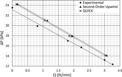
Back to Figure 8, the maximum relative errors in the pressure head (Equation 5(5) $e_p=|\frac{\mathrm{\Delta }{P}_{\mathrm{n}\mathrm{u}\mathrm{m}\mathrm{e}\mathrm{r}\mathrm{i}\mathrm{c}\mathrm{a}\mathrm{l}}-\mathrm{\Delta }{P}_{\mathrm{e}\mathrm{x}\mathrm{p}\mathrm{e}\mathrm{r}\mathrm{i}\mathrm{m}\mathrm{e}\mathrm{n}\mathrm{t}\mathrm{a}\mathrm{l}}}{\mathrm{\Delta }{P}_{\mathrm{e}\mathrm{x}\mathrm{p}\mathrm{e}\mathrm{r}\mathrm{i}\mathrm{m}\mathrm{e}\mathrm{n}\mathrm{t}\mathrm{a}\mathrm{l}}}|.$(5) ) and slope (Equation 6(6) $e_{\mathrm{s}\mathrm{l}\mathrm{o}\mathrm{p}\mathrm{e}}=|\frac{{\mathrm{s}\mathrm{l}\mathrm{o}\mathrm{p}\mathrm{e}}_{\mathrm{n}\mathrm{u}\mathrm{m}\mathrm{e}\mathrm{r}\mathrm{i}\mathrm{c}\mathrm{a}\mathrm{l}}-{\mathrm{s}\mathrm{l}\mathrm{o}\mathrm{p}\mathrm{e}}_{\mathrm{e}\mathrm{x}\mathrm{p}\mathrm{e}\mathrm{r}\mathrm{i}\mathrm{m}\mathrm{e}\mathrm{n}\mathrm{t}\mathrm{a}\mathrm{l}}}{{\mathrm{s}\mathrm{l}\mathrm{o}\mathrm{p}\mathrm{e}}_{\mathrm{e}\mathrm{x}\mathrm{p}\mathrm{e}\mathrm{r}\mathrm{i}\mathrm{m}\mathrm{e}\mathrm{n}\mathrm{t}\mathrm{a}\mathrm{l}}}|.$(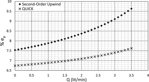6) ) are found to be 9.63 and 5.47% for the second-order upwind model and 7.62 and 5.87% for the QUICK model, respectively. Moreover, Figure 9 illustrates the variation of the pressure head relative error along the entire range of the performance curve. Noticeably, the numerical error increases with the flow rate; this is mainly attributed to the increased numerical diffusion at higher Reynolds numbers. Moreover, the QUICK scheme did not provide a substantial improvement over the second-order upwind scheme using the present grid. Furthermore, the QUICK scheme posed an increased numerical toll on the overall computational cost compared with the second-order upwind scheme. This is mainly attributed to nonlinear instabilities triggered by applying a high-order upwinding scheme (such as QUICK) to a three-dimensional turbulent flow – such behavior was reported in Patel et al. (1987) and ANSYS (2011). Finally, results reported in what follows are for the QUICK scheme due to its superior performance as discussed previously.

Figure 9. Relative error in pressure difference ($e_p$) versus flow rate (Q).

4. Discussion of results

In what follows, the following zones of the dual-seal cartridge are illustrated: the outboard seal; the inboard seal; the pumping ring; and the outlet port. Figure 5 represents the simulated barrier fluid domain in the MPW-RO cartridge indicating the characteristic dimensions involved later on in the following sections.

4.1. Outboard seal

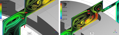
The outboard seal is directly projected onto the barrier fluid inlet port and is located at the suction side of the pumping ring, as illustrated by zone ‘c’ in Figure 5. Figure 10 displays the projected velocity vectors and three-dimensional streamlines in the proximity of the outboard seal. As can be observed in the figure, the barrier fluid enters from the inlet ‘1’ and approach the stationary ‘2’ and rotating ‘3’ rings of the outboard-seal, indicating continuous replacement of the barrier fluid at the outboard-seal proximity.

Figure 10. Projected velocity vectors and three-dimensional streamlines in the vicinity of the outboard seal.

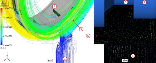
Moreover, rotation of the pumping ring ‘4’ is found to cause the inflow to revolve ‘5’ prior to entering the pumping ring. Furthermore, it can also be seen that the flow reversal from the pumping ring side causes the internal leak ‘6’ to take place. 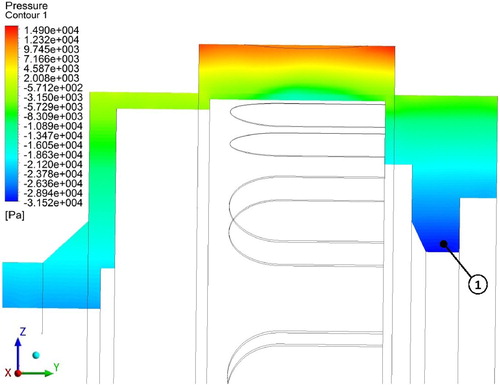For this reason, the tangential velocity radial profiles ($v_{\theta }$ versus $r/R_3$) are plotted in Figure 11 at the following consecutive slices in the perpendicular to the rotation axis: $\frac{y-Y_1}{Y_2-Y_1}=[10\to 70]\mathrm{\%},$ where $Y_1$, $Y_1$ and $R_3$ are the lengths shown in Figure 5. Evidently, this tangential motion of the inlet flow approaching the pumping ring, namely pre-rotation, adversely affects the pumping ring's performance in two aspects. Firstly, it lowers the flow capacity as it reduces transport efficiency due to the increased hydraulic losses/resistance, especially considering the longer path the fluid has to travel from the inlet to the pumping ring. Secondly, the centrifugal action of this pre-rotation effect leads to fluid pressure reduction towards the center of rotation, as can be validated by the pressure contours plotted in Figure 12. Consequently, such a reduction of pressure due to the pre-rotation effect might promote cavitation due to vapor formation, especially at operation conditions entailing elevated temperatures and rotational speeds. In fact, the pre-rotation phenomenon is common in a number of fluid machinery applications such as centrifugal pumps (Breugelmans & Sen, 1982) where it also influences the angle of attack on impeller blades. Finally, it is noteworthy, however, to illustrate that cavitation is also influenced by the pressure setting of the accumulator of the barrier fluid loop.

Figure 11. Tangential velocity ($v_{\theta }$) profiles across the vicinity of the outboard seal ($r/R_3$) at various axial cross sections.

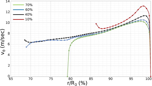
Figure 12. Pressure contours on the Y–Z-plane.

4.2. Pumping ring

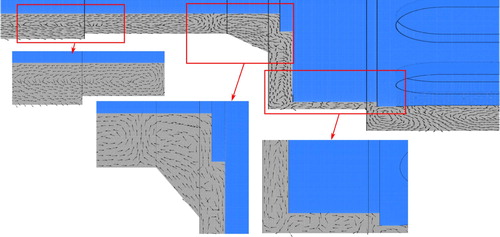
Barrier fluid flow through the slots of the pumping ring is found to be of a complex nature, characterized by three-dimensional combinations of violent swirling flows. Figure 13 shows an illustrative schematic for the pumping ring simulated. Moreover, Figure 14 illustrates two-dimensional streamlines on an axial plane passing by the middle of one slot of the pumping ring. The figure visualizes flow orientation from and to a single groove of the MPW pumping ring. Noticeably, some of the streamlines are discontinuous, as marked by the red arrows in the subfigures. This is attributed to two factors: first, limitation of the visualization software ANSYS CFD-Post^®, as flow field variables in each meshing block are drawn separately and then joined/linked together by means of interface boundary condition – this was also reported by some other users in some online forum discussions such as ANSYS CFD-Post Forum (2013) and ANSYS Forum (2014); the second is the fact that surface streamlines are calculated by integration over the velocity vector field, leading to discontinuity of streamlines due to stagnation points and the accumulation of numerical errors specially when severe swirls and flow separations are present. This might be alleviated by calculating the streamlines by solving the transport equation for an advected scalar quantity C as follows: (7) $\overrightarrow{u}.\mathrm{\nabla }C=u_x\frac{\mathrm{\partial }C}{\mathrm{\partial }x}+u_y\frac{\mathrm{\partial }C}{\mathrm{\partial }y}=0,$(7) where C is constant along a streamline. A similar approach was investigated by Hafez and Wahaba (2004) for a cylindrical coordinate system. However, for this to be implemented, some changes to the underlying code being used need to be made, which is beyond the scope of the present study.

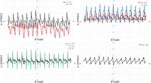
Figure 15 shows projections of the velocity vector field onto an axial mid-plane to a slot of the pumping ring at the slot's axial open end (a) and circumferential end (b), as labeled on the figure. First of all, it is clear from subfigure (a) that the velocity vectors indicate in and out axial flow of the groove as marked by the bold red arrows on the figure. To visualize this variation of the axial flow direction quantitatively, the axial velocity component ($v_y$) is plotted at the axial open end of the slots along the entire circumference of the pumping ring as shown in Figure 16 for the following range: $\frac{r-r_i}{r_o-r_i}=[3.3\to 92.6]\mathrm{\%},$ where $r_i$ and $r_o$ equal $D_i/2$ and $D_o/2$ shown in Figure 13, respectively. Figure 16 indicates that the axial velocity oscillates between positive and negative values implying out and in flow, respectively. Moreover, it can be seen clearly that the axial velocity profiles have an angular periodicity, implying that the flux is periodic and proportional to the number of pumping grooves. Noticeably, at lower values of $(r-r_i)/(r_o-r_i)$, negative values of axial velocity (i.e. inflow) dominate, while at higher values, positive values of axial velocity (i.e. outflow) from the grooves outweigh inflow. This implies that mixed in–out flow is present, to and from the axial open end of the slots. Therefore, to find the new flow direction, the axial velocity component $v_y$ is integrated along the area and the net flow rate is found to be entering the pumping ring, implying that the axial open end of the grooves can be considered the suction side of the pumping ring.

Figure 13. Characteristic dimensions of the MPW ring.

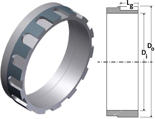
Figure 14. Two-dimensional surface streamlines at a slot's mid-plane of the MPW pumping ring.

Secondly, the circumferential end of the slots of the pumping ring, shown by subfigure (b) of Figure 15, is investigated. Again, mixed in–out radial flows take place as marked by the the red labels on the subfigure. For a quantitative sense, the radial velocity component ($v_r$) is plotted at the circumferential end of the slots, along the circumference of the pumping ring. Moreover, this velocity profile is plotted at the following x–z slices along the length of the slot as shown in Figure 17 for the following range: $L_g=[0\to 100]\mathrm{\%},$ where $L_g$ is the slot length, illustrated in Figure 13. Figure 17 shows positive and negative values of the radial velocity components, implying outflows and inflows to the slots, respectively. Moreover, it can be seen clearly that the radial velocity profiles have an angular periodicity, implying that the flow at the ring's circumference is periodic and proportional to the number of slots, similar to that observed earlier in the axial velocity components of Figure 16. Furthermore, it is observed that, at the beginning of the slots (e.g. $[0,1.3]\mathrm{\%}{L}_g$), negative values of the radial velocity dominate, implying net inflow. While for the range of $[12\to 50]\mathrm{\%}{L}_g$, the velocity values fluctuate around zero. After that, in the range $[62,88]\mathrm{\%}{L}_g$, the net value is positive, implying outflow from the pumping ring. Finally, at the end of the pumping groove, the velocity values decrease and fluctuate around zero for a second time. For this reason, the radial velocity components are integrated over the entire circumferential surface along $L_g$ and the net flow is found to be positive (i.e. net outflow), implying that the circumferential end of the slots can be considered to be the delivery side of the pumping ring.Finally, Figure 18 displays the pressure contours on the surface of the pumping ring. Noticeably, the walls are not aligned with the flow direction, which leads to the formation of a high-pressure stagnation point and a low-pressure separation zone – highlighted by points ‘1’ and ‘2’ in Figure 18, respectively. This also leads point ‘2’ to trigger cavitation at elevated temperatures and speeds.

Figure 15. Projected velocity vectors onto a slot's mid-plane of the MPW pumping ring.

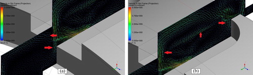
Figure 16. Axial velocity components ($v_y$) plotted at a slot's axial open end for several radii.

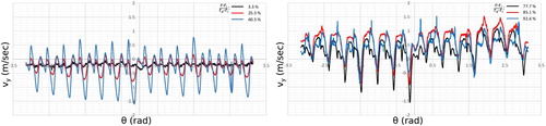
Figure 17. Radial velocity ($v_r$) profiles along the circumferential direction, for several sections along the slot length ($L_g$).

4.3. Inboard seal

The boundaries of the present numerical model are expanded to include inboard sealing faces, which were not included in the previous model of Warda et al. (2015). Figure 19 displays projected velocity vectors and two-dimensional surface streamlines in the region of the inboard seal (zone ‘a’ in Figure 5). The figures show that closed barrier fluid circulation occurs in the region of the inboard seal, resulting in a nearly zero flow rate toward the pumping ring zone. Consequently, the portion of barrier fluid in this zone is trapped and will not be regenerated. This leads to a higher concentration of contaminants, elevated temperature operation and a lower mean time between failures (MTBF) since the fluid in this zone in not being flushed properly. This is usually dealt with in dual seal cartridges by the use of ‘deflector baffles’ to ensure that closed separations in such zones are avoided. See Bloch (2017a) for an example of such designs.

Figure 18. Pressure contours on the MPW walls.

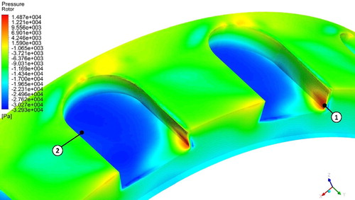
Figure 19. Circulation of barrier fluid at the inboard seal region (zone ‘a’ in Figure 5) represented by two-dimensional projected velocity vectors.

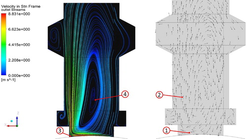
4.4. Outlet port

Figure 20 represents barrier fluid exiting the dual-seal cartridge through the radial outlet port. Obviously, the outlet port is not oriented with the flow direction in the gland. The figure shows that the flow at point ‘1’ is deflected to the point ‘2’ after bouncing off the wall of the outlet port at point ‘3’. This clearly leads to the formation of the large separation zone labelled by point ‘4’ in the figure. Consequently, such a formation partially blocks the outlet port, throttling down flow capacity and increasing hydraulic losses. Even though one could propose here that a streamlined outlet with the expected incident flow should be used, such as the volute casing of centrifugal pumps, this is not simply the case here since the geometry needs to be symmetrical in both directions of rotation to retain bi-directionality of the cartridge. For instance, another variant of the present seal was experimentally investigated by Warda et al. (2018b), wherein the outlet port was tangentially oriented. As expected, a significant increase in the flow rate was observed.

Figure 20. Two-dimensional streamlines and normalized velocity vectors at the outlet port of the cartridge.

5. Concluding remarks

In the present study, a comprehensive evaluation of barrier fluid flow through a typical industrial dual mechanical seal cartridge was presented. For this reason, a numerical model was constructed and validated using the available experimental observations. The study investigated a modified paddle wheel cartridge with radial inlet and outlet ports, whichis classified as a bi-directional radial-flow design. Such a design is distinguished by two major merits in comparison with most other axial-flow designs (e.g. pumping scrolls). The first is the ability to be used in applications where the direction of shaft rotation is expected to vary, which is mainly attributed to the symmetry of the design of the sealing cartridge. The second advantage is that the clearance between the pumping ring and the surrounding gland is greater, which makes it a practical choice for applications where shaft deflections are expected (Bloch, 2017b). However, this increased clearance is a prominent disadvantage from a hydraulic perspective owing to fluid recirculation causing internal leaks. Moreover, the numerical observations of the present study revealed other hydraulic disadvantages that are summarized as follows.

• A relatively large swirling flow took place in the clearance around the region near the outboard seal, consequently reducing the pumping efficiency due to the increased losses. Moreover, this pre-rotation effect caused the pressure to reduce toward the center of rotation; making this design more prone to cavitation, especially at elevated working temperatures and rotational speeds.

• The design of the pumping ring is relatively bluff , leading to a number of adverse consequences. Mixed-flow nature at both the suction and delivery sides of the pumping ring is one example. Another example is the formation of stagnation points on the leading edges of the pumping slots. Moreover, the formation of a low-pressure separation zone on the trailing side of the pumping slots make it a potential cavitation-triggering zone in more severe operating conditions.

• Flow at the inboard-seal region is trapped, forming closed-loop swirling flow. This indicates poor barrier fluid regeneration in this region and, as a consequence, it is expected to be a zone of elevated temperature and contaminants. This might be avoided by the use of ‘deflector baffles’ such as in Bloch (2017a).

• A relatively large separation zone forms at the outlet port owing to the lack of alignment of the outlet port with the expected direction of incident flow. This in turn reduces the hydraulic efficiency and bottlenecks the pumping capacity.

The work presented here forms only a single step of many to come. Above all, the following adaptations and directions should be tested.

• In light of the observations made in the present study, work is in progress investigating a number of design modifications in the following areas: the hampering of pre-rotation at the suction side of the pumping ring (point ‘1’ in Figure 12); groove profile modification to mitigate severe separations (points ‘1’ and ‘2’ presented in Figure 18); flow redirection toward the inboard seal to improve barrier fluid renewal (Figure 19); and outlet port geometry to avoid severe separation (points ‘3’ and ‘4’ in Figure 20) by being more aligned with the exit flow from the pumping ring.

• The pumping ring motion was modeled using the MRF approach, which is a steady-state frozen-rotor approximation producing a time-averaged solution. One major drawback of this is the averaging of the unsteady rotor–stator interactions between the pumping ring and the surrounding gland, such as the proximity of a pumping groove to the outlet port. For this reason, a transient dynamic mesh approach should be investigated such as the sliding mesh (SM) approach to catch such transient interactions between moving and stationary parts.

• The influence on the accuracy of the predicted hydraulic performance curves of higher fidelity turbulence models, such as the Reynolds stress model (RSM) (Launder et al., 1975), should be investigated. However, a scale-resolving model such as large eddy simulation (LES) is expected to have a significant computational cost for such a an industrial flow with high Reynolds numbers and, therefore, should be used locally rather than globally.

• Even though the computational grid was significantly improved compared with previous models and relatively good agreement with experimental observations was achieved, the mesh needs further enhancements to model the wall boundary layer properly. Despite the flow being highly inertial and swirl dominated, the wall diffusion should still be properly modeled by implementing an appropriate number of grid inflation layers next to the bounding walls, which was beyond the reach of the computer used in the present study owing to the considerable computational cost.

Nomenclature

$\mathrm{A}\mathrm{P}\mathrm{I}$	=	American petroleum institute
$\mathrm{M}\mathrm{P}\mathrm{W}$	=	modified paddle wheel
$\mathrm{M}\mathrm{R}\mathrm{F}$	=	multiple reference frame
$\mathrm{M}\mathrm{T}\mathrm{B}\mathrm{F}$	=	mean time between failures
$\mathrm{R}\mathrm{O}$	=	radial outlet
$\mathrm{R}\mathrm{I}$	=	radial inlet
$\mathrm{P}\mathrm{T}$	=	pressure transmitter
$\mathrm{T}\mathrm{T}$	=	temperature transmitter
$\mathrm{M}\mathrm{F}\mathrm{M}$	=	mass flow meter
$\mathrm{S}\mathrm{F}\mathrm{I}$	=	static frequency inverter
$\mathrm{Q}\mathrm{U}\mathrm{I}\mathrm{C}\mathrm{K}$	=	quadratic upstream interpolation for convective kinematics
$\mathrm{S}\mathrm{I}\mathrm{M}\mathrm{P}\mathrm{L}\mathrm{E}$	=	semi-implicit method for pressure linked equations
$\mathrm{G}\mathrm{C}\mathrm{I}$	=	grid convergence index
$\mathrm{S}\mathrm{D}$	=	Standard deviation
$v_r$	=	radial velocity component
$v_y$	=	axial velocity component
$v_{\theta }$	=	tangential velocity component
C	=	a convected scalar quantity
k	=	turbulence kinetic energy
ϵ	=	turbulence dissipation rate
ρ	=	density
μ	=	molecular viscosity
P	=	static gauge pressure
$u_i$	=	Cartesian velocity components
${\tau }_{\mathrm{t}\mathrm{u}\mathrm{r}\mathrm{b}}$	=	turbulence stress tensor
$N_i$	=	number of elements for the $i^{th}$ grid
${\varphi }_i$	=	solution variable for the $i^{th}$ grid
$r_{ij}$	=	grid refinement ratio $N_j/N_i$
p	=	apparent order of convergence
${\varphi }_{\mathrm{e}\mathrm{x}\mathrm{t}}^{21}$	=	extrapolated variable
$e_a^{21}$	=	approximate relative error
$e_{\mathrm{e}\mathrm{x}\mathrm{t}}^{21}$	=	extrapolated relative error
${\mathrm{G}\mathrm{C}\mathrm{I}}_{\mathrm{f}\mathrm{i}\mathrm{n}\mathrm{e}}^{21}$	=	fine-grid convergence index
$e_p$	=	pressure difference relative error
$e_{slope}$	=	relative error in slope
$P_{\mathrm{t}\mathrm{g}}$	=	total gauge pressure
$P_{\mathrm{i}\mathrm{g}}$	=	initial gauge pressure
$m^{\cdot }$	=	mass flow rate
$U_{\mathrm{m}\mathrm{f}}$	=	experimental mean flow velocity
$A_{\mathrm{i}\mathrm{n}\mathrm{l}\mathrm{e}\mathrm{t}}$	=	inlet-port area

Disclosure statement

No potential conflict of interest was reported by the authors.

References

- Akbarian E., Najafi B., Jafari M., Faizollahzadeh Ardabili S., Shamshirband S., & Chau K.-w. (2018). Experimental and computational fluid dynamics-based numerical simulation of using natural gas in a dual-fueled diesel engine. Engineering Applications of Computational Fluid Mechanics, 12(1), 517–534. https://doi.org/10.1080/19942060.2018.1472670
- ANSYS (2011). Ansys fluent 14.0: User's guide (pp. 1316–1317). https://www.scribd.com/doc/140163383/Ansys-Fluent-14-0-Users-Guide
- ANSYS CFD-Post Forum (2013). Surface and 3D streamlines difference. https://www.cfd-online.com/Forums/cfx/115182-cfd-post-surface-3d-streamlines-difference.html
- ANSYS Forum (2014). Discontinuous contour at interface. https://www.cfd-online.com/Forums/cfx/145319-discontinuous-contour-interface.html
- API (2012). Pumps – shaft sealing centrifugal and rotary pumps (4th ed.). API standard 682.
- Blaber J. A. (2003). Training module TM-070. John Crane EAA Training and Development Group. Manchester, UK.
- Bloch H. P. (2017a). Subject category 21 – mechanical seals. In H.P. Bloch (Ed.), Petrochemical machinery insights (pp. 263–300). Butterworth-Heinemann. http://www.sciencedirect.com/science/article/pii/B9780128092729000219; https://doi.org/10.1016/B978-0-12-809272-9.00021-9
- Bloch H. P. (2017b). Subject category 26 – organizational issues. In H.P. Bloch (Ed.), Petrochemical machinery insights (pp. 395–415). Butterworth-Heinemann. http://www.sciencedirect.com/science/article/pii/B9780128092729000268; https://doi.org/10.1016/B978-0-12-809272-9.00026-8
- Breugelmans F., & Sen M. (1982). Prerotation and fluid recirculation in the suction pipe of centrifugal pumps. In Proceedings of the 11th turbomachinery symposium (pp. 165–180). Turbomachinery Laboratories, Texas A&M University. https://doi.org/10.21423/R1DM3B
- Carmody C., Roddis A., Amaral T., & Schurch D. (2007). Integral pumping devices that improve mechanical seal longevity. In 19th international conference on fluid sealing (pp. 235–247). BHR group conference series publication.
- Celik I. B., Ghia U., Roache P. J., Freitas C. J., Coloman H., & Raad P. E. (2008). Procedure for estimation and reporting of uncertainty due to discretization in CFD applications. Journal of Fluids Engineering, 130(7), Article ID 078001. https://doi.org/10.1115/1.2960953
- Deng E., Yang W., Deng L., Zhu Z., He X., & Wang A. (2020). Time-resolved aerodynamic loads on high-speed trains during running on a tunnel–bridge–tunnel infrastructure under crosswind. Engineering Applications of Computational Fluid Mechanics, 14(1), 202–221. https://doi.org/10.1080/19942060.2019.1705396
- Forsthoffer M. S. (2017). Pump mechanical seals. In Forsthoffer's more best practices for rotating equipment (pp. 403–432). Butterworth-Heinemann. http://www.sciencedirect.com/science/article/pii/B9780128092774000085; https://doi.org/10.1016/B978-0-12-809277-4.00008-5
- Hafez M., & Wahaba E. (2004). Incompressible viscous steady flows over finite plate and rotating cylinder with suction. Computational Fluid Dynamics Journal, 13(3), 571–584. https://www.researchgate.net/profile/Essam_Wahba/publication/305000400_Incompressible_viscous_steady_flows_over_finite_flat_plate_and_rotating_cylinder_with_suction/links/577eaf8c08ae69ab8820e824/Incompressible-viscous-steady-flows-over-finite-flat-plate-and-rotating-cylinder-with-suction.pdf
- Launder B. E., Reece G. J., & Rodi W. (1975). Progress in the development of a Reynolds-stress turbulence closure. Journal of Fluid Mechanics, 68(3), 537–566. https://doi.org/10.1017/S0022112075001814
- Launder B. E., & Spalding D. B. (1983). The numerical computation of turbulent flows. In Numerical prediction of flow, heat transfer, turbulence and combustion (pp. 96–116). Elsevier.
- Leonard B., & Mokhtari S. (1990). ULTRA-SHARP nonoscillatory convection schemes for high-speed steady multidimensional flow (NASA Technical Memorandum 102568 ICOMP-90-12). NASA Lewis Research Center. https://pdfs.semanticscholar.org/0802/196cf3d754468b6b37c28d1dc10de38df3e4.pdf?_ga=2.218951697.921977722.1593086048-1053178539.1593086048
- Luan Z., & Khonsari M. (2006). Numerical simulations of the flow field around the rings of mechanical seals. Journal of Tribology, 128(3), 559–565. https://doi.org/10.1115/1.2197845
- Luan Z., & Khonsari M. (2007). Computational fluid dynamics analysis of turbulent flow within a mechanical seal chamber. Journal of Tribology, 129(1), 120–128. https://doi.org/10.1115/1.2401220
- Luo J., Issa R. I., & Gosman A. (1994). Prediction of impeller-induced flow in mixing vessels using multiple frames of reference. In Proceedings of the 8th European conference on mixing (pp. 549–556). Institute of Chemical Engineers Symposium Series. https://www.tib.eu/en/search/id/BLCP%3ACN006796060/Prediction-of-impeller-induced-flows-in-mixing/
- Patel M., Cross M., Markatos N., & Mace A. (1987). An evaluation of eleven discretization schemes for predicting elliptic flow and heat transfer in supersonic jets. International Journal of Heat and Mass Transfer, 30(9), 1907–1925. https://doi.org/10.1016/0017-9310(87)90250-X
- Richardson L. F. (1911). The approximate arithmetical solution by finite differences of physical problems involving differential equations, with an application to the stresses in a masonry dam. Philosophical Transactions of the Royal Society of London. Series A, Containing Papers of a Mathematical Or Physical Character, 210(459–470), 307–357. https://doi.org/10.1098/rsta.1911.0009
- Richardson L. F., & Gaunt J. A. (1927). The deferred approach to the limit. Part I. Single lattice. Part II. Interpenetrating lattices.. Philosophical Transactions of the Royal Society of London. Series A, Containing Papers of a Mathematical Or Physical Character, 226, 299–361.(JSTOR)
- Roache P. J. (1998). Verification and validation in computational science and engineering. Hermosa.
- Smith R. J. (2010). Pressurized dual mechanical seals supporting piping plan developments. In Proceedings of the twenty-sixth international pump users symposium. https://pdfs.semanticscholar.org/4388/ae2ba31d693f30ecce03fb9122014d24ac18.pdf
- Smith R. J. (2014). API type pressurised dual seals – design configurations for contaminated upstream pumping applications. In IMechE fluid machinery congress, 2014, October 6–7 (pp. 33–43). Woodhead Publishing. http://www.sciencedirect.com/science/article/pii/B9780081001097500042; https://doi.org/10.1533/9780081001080.2.33
- Warda, H.A., Adam, I.G., Rashad, A.B., & Gamal-Aldin, M.W. (2018a). Bi-directional integral pumping devices for dual mechanical seals: Influence of mesh type on accuracy of numerical simulations. Alexandria Engineering Journal, 57(4), 3255–3264. https://doi.org/10.1016/j.aej.2017.11.013
- Warda H. A., Adam I. G., Rashad A. B., & Gamal-Aldin M. W. (2016). Effect of kinematic viscosity of barrier fluids on the performance of a bi-directional integrated pumping ring for dual mechanical seals. In ASME 2016 fluids engineering division summer meeting collocated with the ASME 2016 heat transfer summer conference and the ASME 2016 14th international conference on nanochannels, microchannels, and minichannels. American Society of Mechanical Engineers. https://doi.org/10.1115/FEDSM2016-7763
- Warda H. A., Adam I. G., Rashad A. B., & Gamal-Aldin M. W. (2018a). Bi-directional integral pumping devices for dual mechanical seals: Influence of mesh type on accuracy of numerical simulations. Alexandria Engineering Journal, 57(4), 3255–3264. https://doi.org/10.1016/j.aej.2017.11.013
- Warda H. A., I. G. Adam, Rashad A. B., & Gamal-Aldin M. W. (2018b). Integral pumping devices for dual mechanical seals: Hydraulic performance generalization using dimensional analysis. Journal of Engineering for Gas Turbines and Power, 140(8), Article ID 082507. https://doi.org/10.1115/1.4039083
- Warda H. A., Wahba E. M., Rashad A. B., & Mahgoub A. A. (2018). Experimental and numerical investigation of axial single scroll integral pumping devices for dual mechanical seals. Alexandria Engineering Journal, 57(4), 2719–2728. https://doi.org/10.1016/j.aej.2017.10.007
- Warda H. A., Wahba E. M., & Selim E. A. (2015). Integral pumping devices for dual mechanical seals: Experiments and numerical simulations. Journal of Engineering for Gas Turbines and Power, 137(2), Article ID 022504. https://doi.org/10.1115/1.4028384