Prediction of significant wave height; comparison between nested grid numerical model, and machine learning models of artificial neural networks, extreme learning and support vector machines

Abstract

Estimation of wave height is essential for several coastal engineering applications. This study advances a nested grid numerical model and compare its efficiency with three machine learning (ML) methods of artificial neural networks (ANN), extreme learning machines (ELM) and support vector regression (SVR) for wave height modeling. The models are trained by surface wind data. The results demonstrate that all the models generally provide sound predictions. Due to the high level of variability in the bathymetry of the study area, implementation of the nested grid with different Whitecapping coefficient is a suitable approach to improve the efficiency of the numerical models. Performance on the ML models do not differ remarkably even though the ELM model slightly outperforms the other models.

KEYWORDS:

• Numerical modeling
• nested grid
• wind waves
• machine learning
• extreme learning machines
• deep learning

1. Introduction

Reliable estimation of wave height in coastal waters can provide useful information for many different practical applications in coastal engineering, environmental monitoring, coastal protection, and marine transportation. Significant wave height is considered as a vital parameter in the design and construction of coastal protection structures, sediment transport, and port locating and development. Several parameters can affect wave height in nearshore and offshore areas such as water depth, swells, shoaling, refraction and diffraction, storms and winds (Malekmohamadi et al., 2011). Generally speaking, methods employed to simulate wave characteristics can be recognized in two main categories of numerical wave models and regression/ empirical techniques. Concerning wave simulation with numerical models, it is not an easy task to measure all of these variables for different points. Also, changing local conditions affecting the physics of the phenomena should be considered in the modeling procedure to minimize the errors. On the other hand, regression-based models are mainly developed to find a statistical relationship between the target variable here means wave characteristics and some influencing variables such near-surface wind speed, wind blowing direction, mean sea level pressure among the others. Artificial intelligence techniques such as artificial neural network (ANN), adaptive neuro-fuzzy inference systems (ANFIS), support vector machine (SVM), and k-nearest neighbor (KNN) can be considered as nonlinear regression-based models which are black-box models to find a relationship between input and target variables without providing exact mathematical relationships and physics of the phenomena (Mosavi et al., 2018). Both numerical and regression-based models have their own pros and cons. For example, numerical models inherently have higher computational cost and complexity than the statistical models. On the other hand, they are consistent with the physics of the phenomena and consider governing equations and boundary conditions for modeling procedures. However, they usually require a lot of input variables to tune the numerical model and also to meet special conditions. Thus, developing models with reliable estimation of wave characteristics using only a limited number of input variables is of great interest.

Numerical models due to their consistency with the physics of the phenomena have been widely used for wave simulations. Among different models developed for this purpose such as MIKE, WAM, WAVEWATCHIII, the Simulating Waves Nearshore (SWAN) developed at Delft University of Technology as a third-generation wave model has attracted great popularity and has been widely used for wave simulation for different regions. Results of the wave model with available measured wave data for different study areas demonstrated that the proposed model can be successfully employed to simulate wave characteristics for coastal engineering applications (Ris et al., 1999). However, dealing with any numerical simulation, calibration of the numerical model play an important role in efficiency and performance of the model. Therefore, prior to serious modelling, the numerical model and the parameters within should be tunes carefully to achieve accurate and reliable results. Moreover, comparing results of the numerical models with those of traditional model can provide overall assessment of the model and conditions.

Machine learning (ML) based models extract mathematical expressions or find empirical relationships between input and target variables from analysis of available time series (Solomatine & Ostfeld, 2008). They have been widely used for real-life applications of different fields such as discharge and river flow prediction (Cheng et al., 2005; Yaseen et al., 2018), evaporation estimation and flood management (Fotovatikhah et al., 2018; Moazenzadeh et al., 2018) and for wind speed prediction (Samadianfardet al., 2020). Artificial neural network (ANN), as a common type model, was widely used for different forecasting applications. Apart from the ANN, other types of soft computing techniques including SVR and ANFIS were also employed for time series simulation and prediction. Malekmohamadi et al. (2011) and James et al. (2018) applied different ML models to predict wave conditions in coastal waters indicating the efficiency of the employed models. Moreover, recently, Anitescu et al. (2019) presented a successful application of ANN to solve the second-order boundary value problem and the results showed that using ANN can lead to remarkable computational savings especially for the non-smooth solutions. Due to inherent simplicity, easily implementation and suitable performance, they are being increasingly in use and attracting more popularities than traditional conceptual models. Extreme learning machines as a more recent version of the ANN have been successfully applied and examined for the forecasting time series in many different applications in hydrology and environmental studies among others. On the other hand, ML-based models can be developed by employing only a limited number of input variables, which are of great importance as the conceptual models require to introduce a large number of variables affecting the target parameter. In this regard, different types of ML-based models based on their performance, complexity, and computational cost have been designed and developed to simulate and predict several different atmospheric, oceanic, environmental and hydrological processes (Alizadeh, Nourani, et al., 2017; Taormina & Chau, 2015; Wang et al., 2009). Dealing with such models there is no need to introduce exact mathematical relationships between input and outputs. The models recognize the relationship through a training procedure and assign appropriate weights indicating the strength of the input variables. For wave modeling purpose, there are two usual approaches which include predicting the wave height using wave height in previous time steps or estimating wave height using wind data as the main driven force.

Similar to numerical models that require calibration data sets to tune the model parameters, the ML-based models also need some data called training data set to set main elements in the structure of the models. For example, the number of iteration, number of neurons in the hidden layer for ANN models should be tuned appropriately in order to obtain sound predictions of the target variable during the testing period in which it is equivalent to the verification period in numerical models. In the Persian Gulf, Iran, Bushehr and Assulayeh Ports are among the most important ports. The wave records in these two ports obtained from the wave buoys are applied for training and testing the ML-based models. Finally, to overcome limitations of the available studies, the development of a nested grid numerical model to consider local conditions in the modeling procedure and also to evaluate its performance against ML-based models can provide more insights into the manipulation of wave characteristics.

In this study, two types of models including numerical framework using SWAN and ML-based models are applied to estimate wave height in two different points in the Persian Gulf. To establish the numerical model, bathymetry and wind components and for the ML-based models, surface wind speed is considered as input variable and wave height as target variable. To enhance efficiency of the numerical model, a nested grid approach for the selected points are developed subsequent to the primary coarse resolution numerical model to better catch local conditions. Concerning the latter approach, three different ML-based models including ANN, ELM and SVR are developed and their performances for wave height estimation are compared. Finally, efficiency of the ML-based models against the nested numerical model is compared and their advantages and disadvantages are discussed. Rest of the paper is organized as follows. Section 2 describes the study area and datasets, ML-based models, SWAN model and nested grid approach as well as modelling procedures. Results of different models whether the numerical model or the ML-based methods are argued and compared in section 3. Concluding remarks consists the last section of the manuscript.

2. Materials and method

2.1. Study area and data

The study area (Persian Gulf) covers a large area extended from the northwest of the Indian Ocean. Actually, the Gulf has a completely enclosed body except at its eastern part, which in its narrowest part, so-called Hormoz Strait is connected to high seas. Placing between Iranian plateau to the north and Arabian Peninsula to the south (Kamranzad, 2018), it has been surrounded by different countries in which they are under rapid growth in different categories such as population, economic, industry, and subsequently marine transport. Unlike its varying bathymetry and from point by point, which confirms its high level of spatial depth variability, the area generally has a shallow depth with an average depth of 35 m (Emery, 1956) and reaching 90 m in its deepest points. Overall, the shallow waters are usually in the southern stripe of the Gulf, mainly from the coastal areas in Arabian countries, while the deeper waters are in the northern stripe of the Gulf as well as its middle part. The wave data recorded in Bushehr and Assaluye ports during 2008 are employed as target variables in ML-based models. These two ports have been marked in the Persian Gulf map in Figure 1.

Figure 1. Study area.

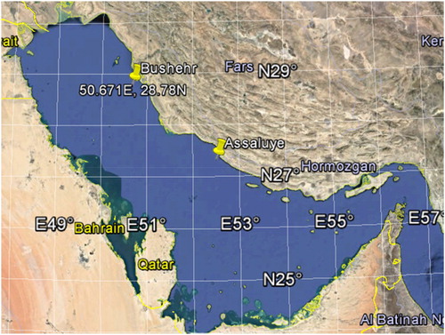
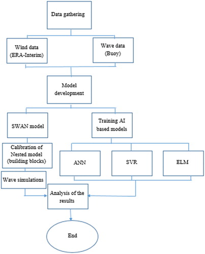
Figure 2. Flowchart of the study.

In this study, the models were forced with surface wind data in 10 m to estimate wave height. Wind data in the Gulf was obtained from ERA-Interim reanalysis data provided by the European Center for Medium-range Weather Forecast (ECMWF). These wind fields with a temporal resolution of 6 h and also with a spatial resolution of 0.5°×0.5° were obtained for the year 2008 as the wave records were available for this period. Statistical analysis of wind and wave data used for this research is presented in Table 1.

Table 1. Statistical analysis for wave and wind data in Bushehr and Assaluye ports.

	Wind speed (m/s)			Wave height (m)
Station	Average	Max	Std	Average	Max	Std
Bushehr	4.40	11.76	2.38	0.55	2.45	0.45
Assaluye	4.35	13.16	2.42	0.45	1.88	0.37

From Table 1, it can be derived that average wave height has higher values in Busher port compared with the corresponding value in Assaluye port. However, the average in wind speed in these two locations does not differ significantly. Therefore, these two places have roughly the same average wind speed but with the different average in wave heights. Therefore, some other parameters are affecting the wave height. The bottom is about 28 and 50 m deep for Bushehr and Assaluye where the buoys were installed. Thus, shoaling can be an effective parameter increasing wave height in Bushehr port. Wave data in Bushehr are changing in a wider range with higher extreme values.

Despite the ML-based models in which only wind data at the forecasting point is fed as the model input, the numerical model require to provide wind data for the whole computational domain. In this study, the wind data from the same source as the ML-based models but covering the whole domain called the Persian Gulf are employed to develop the numerical model.

2.2. ML-based models

2.2.1. Artificial neural network

Artificial neural networks (ANN) at their most common type have three layers as their constituents which each layer is connected to the subsequent one by means of neurons. Generally, they mimic the biologic and natural behavior of human brains which are made of numerous neurons connected together. The first layer called the input layer receives raw data as input variables and transforms them into the hidden layer through the connection between these two layers. In the hidden layer, the main computations are implemented and important relationships and dependency of the variables are extracted, the model is trained based on the available data. The connections between two layers are varied in robustness and weakness while the weight for each parameter or connection is assigned based on the power of the connection. In other words, the most important variable has the highest weight and vice versa. Finally, the nodes in the hidden layer are linked to the output layer determining the value of the target variable. This procedure is a repetitive process that continues for a specified number of iteration or when the performance criteria met. The usual ANN gains a backpropagation algorithm to train the model based on the available input and output records. Generally, a three-layer ANN model in its simplest form can be expressed as: (1) ${\text{o}}_j=\sum _{i=1}^n{\text{β}}_i\text{g}\left({\text{w}}_i{\text{x}}_j+{\text{b}}_i\right)j=1,\dots ,N$(1) where ${\text{x}}_j$ and ${\text{o}}_j$ are the input and output values at node j, $g$ is the activation function in the hidden layer, ${\text{b}}_i$ is the bias of the hidden layer, and n is the number of neurons in the hidden layer. The weights between the input nodes and the ith hidden node and the weight between the ith hidden node and the output nodes are specified with ${\text{w}}_i$ and ${\text{β}}_i$, respectively. It is noted that in this research the log-sigmoid was used as the activation function in the hidden layer.

2.2.2. Extreme learning machine (ELM)

Compared with the ANN models, ELM based models are faster. This technique originally developed by Huang et al. (2004) has been successfully applied for different fields in time series forecasting. Its main advantage over the common ANN models is that it has lower computational cost while it is more efficient in terms of the model generalization. The higher speed in the algorithm implementation is mainly due to its randomly assigning the weights and biases whereas in the ANN models it is carried out through a repetitive process. Moreover, as clear from the name of the algorithm which manipulates extreme values efficiently, the models based on ELM do not suffer from the overfitting problems and also stacking in local minima, which are major concerns dealing with the ANN model. Assuming that there exist $w_i,{\text{β}}_i,b_i$ in which the target variable of N sample ($Y_j$) can be estimated with zero error (i.e. $Y_j=o_j$). Therefore Equation (2) can be rewritten in compact form as: (2) $H\text{β}=Y$(2) (3) $H={\left[\begin{array}{ccc}g\left(w_1.x_1+b_1\right)& \dots & g\left(w_n.x_1+b_n\right)\\ ⋮& \dots & ⋮\\ g\left(w_1.x_N+b_1\right)& \dots & g\left(w_n.x_N+b_n\right)\end{array}\right]}_{N\ast n}$(3) (4) $\text{β}={\left[\begin{array}{c}{\text{β}}_1^T\\ ⋮\\ {\text{β}}_n^T\end{array}\right]}_{n\ast m},Y={\left[\begin{array}{c}{y}_1^T\\ ⋮\\ y_N^T\end{array}\right]}_{N\ast m}$(4) where the output matrix in the hidden layer is denoted by H.

The matrix H can remain fixed by assigning arbitrary values to the parameters at the beginning of learning in the ELM. Therefore, the ELM is trained by finding a least-squares solution $\widehat{\text{β}}$ as: (5) $\begin{array}{rl}& ||H\left(w_1,..,w_n,b_1,..,b_n\right)\widehat{\text{β}}-Y||\\ & =\underset{\text{β}}{min}||H\left(w_1,..,w_n,b_1,..,b_n\right)\text{β}-Y||\end{array}$(5)

Finally, the least square technique can be employed to get the solution for the abovementioned generated matrix. This equation can be written in the general form of: (6) $\widehat{\text{β}}=H^{†}Y$(6) where $H^{†}$ is the Moore–Penrose generalized inverse of matrix H.

2.2.3. Support vector regression (SVR)

Generally, support vector machines have two usual forms appropriate for classification and forecasting. The latter one uses a regression-based method is called support vector regression in which it has more applications in time series manipulation. To train an SVR in its basic form assuming a dataset of $\left\{\right(x_i,y_i){\}}_{i=1}^n$ in which the input and output variables are denoted by x and y and also n represents the sample size, the approach is proceeded to project the input space into an n-dimensional feature space using a nonlinear function ($\varphi \left(x\right)$). The following equation can be applied to formulate the SVR function in its general form (Liu et al., 2014). (7) $f\left(x\right)=\left(w.\varphi \left(x\right)\right)+b$(7)

In which w is the weight vector $w=\left\{w_1,\dots ,w_n\right\}$, and b is standing for the bias. To properly determine the weight and bias in the SVR, a cost function is defined while the traditional models for regression approach were mainly based on the solution of the least square technique to minimize the errors. On the contrary, in SVR, a new loss function known as the ε-insensitive loss function is employed to find the optimum values of bias and the weight vector discussed earlier as (Vapnik, 2013): (8) $L_{\epsilon }\left(f\left(x\right),y\right)=\left\{\begin{array}{ll}|f\left(x\right)-y|-\epsilon & \text{for}|f\left(x\right)-y|\ge \epsilon \\ 0& \text{Otherwise}\end{array}\right.$(8) In which $L_{\epsilon }$ denotes the loss function, y represents the output, and $\epsilon$ is the region of $\epsilon$ insensitivity. Consequently, the regularized risk function (Equation (9)) can be employed to find the weights. (9) $R_{\text{reg}}=C\frac{1}{n}\sum _{i=1}^n{L}_{\epsilon }\left(f\left(x_i\right),y_i\right)+\frac{1}{2}{w}^2.$(9) In which the regularization term and constant are defined as $\frac{1}{2}{w}^2$ and C. However, this equation can be reformatted to establish an optimization problem. As we know, optimization problems are usually recognized by objective cost function and constraints in which are employed to find the best solution where the cost function has its optimum value. In this regard, the following optimization problem can be defined considering the abovementioned equation in which the cost function and constraints are represented as: (10) $\text{minimize}\frac{1}{2}{w}^2+C\sum _{i=1}^n\left({\xi }_i,{\xi }_i^{\ast }\right).$(10) (11) $\text{subject}\text{to}\left\{\begin{array}{c}{y}_i-\left(w.\varphi \left(x_i\right)+b\right)\le \epsilon +{\xi }_i\\ \left(w.\varphi \left(x_i\right)+b\right)-y_i\le \epsilon +{\xi }_i^{\ast }\\ {\xi }_i\ge 0,{\xi }_i^{\ast }\ge 0,i=1,\dots ,n\end{array}\right..$(11)

In which ${\xi }_i$ and ${\xi }_i^{\ast }$ are defined as the positive slack variables measuring the train samples’ deviation outside the $\epsilon$-insensitivity zone. To sum up, with reshuffling the abovementioned equations and functions and computations, the SVR model can be mathematically expressed as (Vapnik, 2013): (12) $f\left(x\right)=\sum _{i=1}^n\left(a_i-a_i^{\ast }\right)K\left(x,x_i\right)+b.$(12) where $a_i$, $a_i^{\ast }\ge 0$ are the Lagrangian multipliers that satisfy the equality $a_i{a}_i^{\ast }=0$; and $K\left(x,x_i\right)$is the kernel function.

2.3. SWAN wave mode

The SWAN (Simulating Wes Nearshore) is a third-generation wave model that is a suitable proxy to model short-crested waves overcoming the drawbacks of the first and second-generation wave models including lack of properly addressing wave generation, wave-wave interactions, and dissipation (Booij et al., 1999). The wave action density spectrum and a Eulerian approach are used to formulate the model. Moreover, wind and boundary conditions are main forcing inputs imposed on the model to simulate wave propagation over arbitrary bathymetry and current fields. Comparing with the other third-generation models, in SWAN model an implicit numerical scheme while the others are based on explicit scheme requiring stability check through Courant number criterion. The process of wind energy transferred to the waves is carried out by mechanisms described by Phillips (1957) and Miles (1957). In brief, considering the spectral action balance equation, the model can be basically formulated in Cartesian coordinates as (Hasselmann et al., 1973): (13) $\frac{\mathrm{\partial }}{\mathrm{\partial }t}N+\frac{\mathrm{\partial }}{\mathrm{\partial }x}{c}_{x}N+\frac{\mathrm{\partial }}{\mathrm{\partial }y}{c}_{y}N+\frac{\mathrm{\partial }}{\mathrm{\partial }\sigma }{c}_{\sigma }N+\frac{\mathrm{\partial }}{\mathrm{\partial }\theta }{c}_{\theta }N=\frac{S}{\sigma }.$(13) in which the wave action density N is defined as a function of relative frequency $\sigma$ and the wave direction $\theta$, $c_x$, $c_y$, $c_{\sigma }$, $c_{\theta }$ are the propagation velocities in x, y, $\sigma ,\theta$ directions. The term S in the right-hand side of the equation is the source terms associated with the generation, dissipation, and nonlinear wave-wave interaction impacts. The source term can be formulated as: (14) $S=S_{in}+S_{nl}+S_{ds,w}+S_{ds,bot}+S_{ds,br}$(14) where the first term is related to input wind which represents the wind energy transfer to the waves, $S_{nl}$ is the corresponding source term for nonlinear wave-wave interactions, and the three last terms in the right-hand side of equation 1(1) ${\text{o}}_j=\sum _{i=1}^n{\text{β}}_i\text{g}\left({\text{w}}_i{\text{x}}_j+{\text{b}}_i\right)j=1,\dots ,N$(1) 4 denote for energy dissipation due to whitecapped, bottom friction, and breaking phenomena, respectively. This study is not aimed to delve into details of the different source terms and further information can be found in Booij et al. (1999), Pallares et al. (2014) and Komen et al. (1984). However, for the model calibration and in order to appropriately tune the parameters, different source terms affecting the model efficiency should be determined carefully. These terms are mainly dependent on the conditionals governing the study area, bathymetry, bed materials and characteristics, and the local climate of winds and waves. For example, for deepwater conditions, white capping is a more influencing parameter while for shallow water conditions, depth induced breaking and friction have more importance on the wave characteristics and energy dissipation.

Dealing with the SWAN model, the nested grid approach is a suitable capability of the model to focus on areas with higher importance or to put a finer mesh-grid over there. Moreover, due to changing bathymetry, tuning a large study area with a unique calibration parameter such as white capping may increase errors to the model simulations. Therefore, through a nested framework, it is possible to define separate areas with different tuning parameters to achieve reliable outputs. To do that, some modifications should be inserted in the subsection of boundary and initial conditions in the model development. Generally, a nested SWAN run is derived from a coarse grid SWAN run. Therefore, the coarse grid SWAN model is firstly run over the whole area with lower spatial resolution and the area of importance is derived from the model. Subsequently, a nested SWAN run will be implemented with the same geographical coordinates as the coarse model but with a much higher number of meshes. Similarly, the parameter of interest such as white capping can be modified in the nested SWAN run.

2.4. Modeling procedure

This study was organized to simulate wave characteristics in two stations in the Persian Gulf by means of artificial intelligence-based methods and also numerical modeling. Dealing with ML-based models, ANN, SVR and ELM models have been taken under consideration. The models were trained using near-surface wind speed as an input variable, and significant wave height was considered as the target variable. ERA-Interim wind data from ECMWF were obtained as input variable and Buoy records at Assaluyeh and Bushehr stations were used as the target variable for the model training and testing purposes. In the three-layer ANN model, the main elements of the network including a number of neurons in the hidden layer, activation function, and training algorithm were set as 2, sigmoid, and Levenberg-Marquardt backpropagation algorithm, respectively. The sigmoid activation function is the most common type function in use for the hidden layer while the hidden layer data are transformed to the output layer by means of a linear function. A number of neurons in the hidden layer were obtained through a trial and error procedure prior to any serious modeling. It is noticed that the ANN model can be trained using different algorithms such as optimization techniques including swarm-based algorithms (e.g. bee algorithm, cuckoo, and imperialist competitive algorithms). However, the Levenberg-Marquardt algorithm is among the most common types and fastest techniques for training ANN models (Alizadeh, Shabani, et al., 2017). The SVR model was developed according to its library in MATLAB and the default values were set for the model. However, other kernel functions such as Gaussian function can be tried as the default kernel function is linear. Similar to the ANN model, the ELM model components of a number of hidden neurons and activation functions were set as 10 and sigmoid, respectively. On the other hand, SWAN was used for numerical modeling feeding with bathymetry and wind data as input. Due to deep water conditions at the location of wave Buoys, the model calibration was carried out using white capping coefficient. Other parameters were initiated with the default values. In this regard, a two dimensional model at the non-stationary state and spherical coordinate were developed. The coarse model was initiated with a spatial resolution of 0.1 times 0.1 degrees and a computational time step of 30 minutes. For the nested SWAN run, specifications of the spatial and temporal resolution were higher to achieve higher accurate simulations. To do that, the building blocks have been calibrated gaining local conditions but still, whitecapping was considered as the main factor because of governing deepwater conditions (Pallares et al., 2014). However, the temporal resolution of the model in the nested grid was assumed about 10 min and also the spatial grids were constructed with half of the coarse resolution grid as 0.05. Finally, outputs of the different models are evaluated at the two stations. The modeling procedure can be summarized as a flowchart presented in Figure 2.

3. Results and discussion

3.1. ML-based models

Several models using the ML approach were developed to estimate wave height in two stations in the Persian Gulf. In this regard, 6-hourly wind data were employed as input variables for the models’ development. Three different types of ML have been constructed and trained with the available wave measurements. 70% of the data set were applied to train the models, and 30% remained as testing data. The performance of different models during the testing period is given in Table 2.

Table 2. Wave results for Bushehr and Assaluye ports.

	Bushehr Port			Assaluye Port
	RMSE	MAE	R^2	RMSE	MAE	R^2
ANN	0.3	0.22	0.75	0.34	0.25	0.2
ELM	0.29	0.21	0.75	0.34	0.25	0.21
SVR	0.34	0.24	0.71	0.35	0.25	0.24

According to Table 2, the ELM model is superior over the ANN and SVR models for both stations. Moreover, the models provide more accurate predictions for wave height in Bushehr Port compared with Assaluye Port. On the other hand, results of statistical analysis during 2008 indicate that wind waves in Bushehr Port have higher average and extreme values. Generally, the performance of all the models (ANN, ELM, and SVR) is near to each other. It means, trying with different ML-based models with similar input variables or similar methodology does change the efficiency of the proposed models remarkably. The results of different models versus measured values of wave height in Bushehr Port are depicted in Figure 3.

Regarding Figure 3, a relatively high correlation among the observed and estimated values of wave height can be observed. For all the three models, the high values of the determination coefficient (R²>0.7) demonstrate the efficiency of the developed models for wave height estimation. However, it is clear from the figure that these models underestimate the wave height in the station. For example, the ELM estimation of the wave with a height of 2.5 does not reach 2 m. A similar comparison for the other models can be derived. The outputs of the models for Assaluye Port are illustrated in Figure 4.

Figure 3. Predictions of ML-based model for wave height in Bushehr Port.

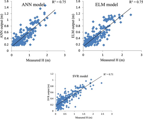
Figure 4. ML based models’ predictions for wave height in Assaluye Port.

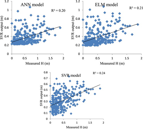
The results in Figure 4 show a relatively low correlation between observed and estimated values of wave height. Moreover, the models underestimate wave height in the range from average to high values. A comparison between the performances of the models in two stations, it can be found that the models are frequently superior in Busher Port than Assaluye Port in terms of mean absolute error (MAE) and root mean square error (RMSE), and R² as well. These results have been obtained while for both stations, the models’ input variable and specifications were the same. Thus, for wave height estimation in Assaluye Port, more actions should be taken under consideration to improve the models’ predictions. The ML-based models in Assaluye Port have deficiency especially in predicting extreme values while they predict the extreme value of 2 m about 1 m. According to Figures 3 and 4, it is obvious that the ANN and ELM have a roughly similar performance and also a range of simulations as their vertical axis indicating predicted wave height are the same. On the other hand, the SVR model has a frequently lower value of predicted wave heights which implies it generally underestimates wave height for both locations. All in all, it can be derived that the ELM model slightly outperforms the other ML-based models explored in this study. Considering the ELM model as the model with the best performance, the time series of wave height for measured and predicted values are illustrated for Busher Port in Figure 5 to provide more comparisons. It is noticed that the time series forecasts are depicted only for ELM model simulations as it outperforms the SVR model. Moreover, its predictions are almost the same as the predictions obtained from the ANN model.

Figure 5. ELM outputs for wave height in Bushehr Port.

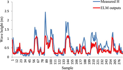
In Figure 5, it is observed that the ELM model generally provides a reliable estimation of wave height from low to average and average to high values of the target variable. Moreover, it has the same distribution and variation of the original data. In other words, the highest values of wave height for measured and predicted models are related to the same time. It is of great interest in wave simulation. Thus, the ELM model provides sound predictions for wave height in Bushehr Port. However, for extreme values, slightly underestimation can be found for the ELM model. A similar illustration is given for Figure 6 in Assaluye Port.

Figure 6. ELM outputs for wave height in Assaluye Port.

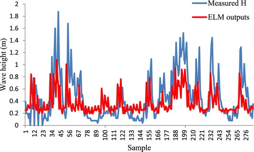
The results of Figure 6 reveal that the ELM model in Assaluye Port generally overestimate low and average values of wave height while it underestimates the high values. Also, the predictions in some points show some inconsistency with the measured values. Therefore, it is recommended to include more input variables to improve the model efficiency. Moreover, applying data pre-processing or post-processing of the model outputs can be helpful to achieve better predictions of the wave height in the region.

3.2. Numerical model

The second approach to simulate significant wave height is the SWAN model using based on finite difference numerical method to discrete wave action balance equation. The model was first to run on the whole domain in a coarse resolution, and the nested model obtained from that was used to finer resolution modeling. Moreover, due to wide variation in the bathymetry of the study area, the calibration for each station may differ as the source term can be varied, or due to variable conditions, different Whitecapping coefficient is required to apply for each station. The nested SWAN was run for two stations during 2008. Half of the data were used for the model calibration, and the 50% rest of the data were used in the verification period. Aside from Whitecapping coefficient which employed as the main variable for the model calibration, the other dissipation coefficient explained in source terms such as depth induced breaking and bottom friction were supposed as the model defaults. The results related to significant wave height simulated by the model against measured data and for verification period are illustrated as Figure 7.

Figure 7. Simulated wave height versus measured wave in Bushehr and Assaluyeh.

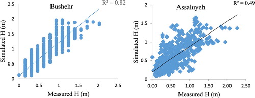
As observed in figure 7, good agreement and consistency can be found among measured and simulated wave heights at both stations. However, the results for the Bushehr station showed a higher correlation than the results in Assaluyeh. The scatter plot depicting the results for Bushehr station has a coefficient of determination higher than 0.8 in which it represents a high correlation between measured and simulated wave height. For the other station, the coefficient is less than 0.5 that shows the model falls to estimate wave height accurately. Generally, it can be found that the model for Assaluyeh station underestimates wave height, especially for peak waves. For example, the wave with a height about 2.5 m is estimated at less than 2 m. A similar conclusion for Bushehr station can be derived but the difference between measured and simulated peak waves in this station is frequently lower than the other station. To provide more insights on the computed values for the numerical models, Figure 8 gives simulated wave height for the verification period against measured wave height based on their temporal order.

Figure 8. Illustration of simulated and measured wave heights based on their temporal order.

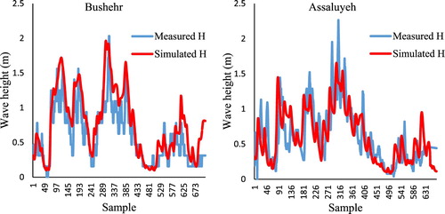
According to Figure 8, simulated waves at Bushehr station have good agree of similarities with those of the corresponding measured wave heights. However, the general trend indicates that the simulated waves slightly overestimate recorded waves by the Buoy. On the other hand, wave height at Assaluyeh station are higher than those of the simulated values. The model underestimation for this station is more highlight for peak waves than the mean values. Overall, SWAN model provides suitable estimations for both stations even though some improvement on the model should be carried out to achieve more reliable results. Moreover, comparing the results for different stations shows high spatial variability in the model performance where for some points the model underestimates and for the other points it overestimates wave height. To provide a quantitative analysis of the model performance and compare it with the ML-based models, Table 3 gives the results of error measures for the numerical model at both stations.

Table 3. Performance of the numerical wave model for the two stations.

Station	RMSE	MAE	R^2
Bushehr	0.273	0.205	0.815
Assaluyeh	0.289	0.217	0.485

Regarding Table 3, the model has roughly similar performance for both stations in terms of RMSE and MAE while the values of coefficient of determination differ from each other significantly. Thus, considering R² as the only criterion for evaluating the performance of the model is not reliable, and some other measures should account for it. However, model deficiency for extreme values may change the coefficient of determination remarkably while the model provides suitable estimations for other values. Comparing the performance of the numerical model with those of ML-based models reveal that the numerical model outperforms the ML-based models in terms of coefficient of determination. However, the difference is not remarkable in terms of RMSE and MAE but the numerical model slightly has lower RMSE and MAE than the ML-based models. Therefore, the results of ML-based models and the numerical model are comparable and they can be employed alternatively based on the purpose of the study and available datasets.

4. Conclusions

Sound prediction of significant wave height is considered as a key element for the design and construction of coastal protection structures, marine transportation, and offshore industry. In this study, three different models including ANN, ELM, and SVR as well as the SWAN model as a numerical approach are developed. In this regard, ML-based models were trained using ERA-Interim wind data near the station and wave data recorded by the Buoys. To establish the numerical model, bathymetry and near-surface wind components from the same source as the ML-based models were employed for the model calibration. For the ML-based model and numerical model, 70% and 50% of the datasets for two stations of Bushehr and Assaluyeh in the Persian Gulf were used for the model training and calibration, respectively.

Comparing the results of the different ML-based models indicated that ANN, ELM and SVR models generally provide similar predictions for both stations. However, the ELM slightly outperforms the others. The ML-based models in Bushehr Port provide reliable predictions for wave height and good consistency with the observed values. However, for the Assaluye Port, the models are not as accurate as desirable and more actions should be taken under consideration in order to improve the model efficiency. The models for Busher Port predict low to high values of the wave height with acceptable efficiency but still, they underestimate extreme values. For the other station, the models overestimate low to average values and underestimate extreme values. Therefore, the models for both stations have a deficiency in predicting extreme values. In this regard, more effective input values and also linking these models with data pre-processing techniques can be considered as efficient.

Simulations obtained from the numerical model demonstrated that the model has a suitable capability to provide sound estimations of the wave height for both stations. For the Bushehr, the model during the verification period has relatively low values of root mean square error and mean absolute error and also high correlation all indicating the efficiency of the model. Moreover, the model properly simulated extreme values even though for some cases there was small inconsistency. However, for the Assaluyeh station, the model has a relatively low value of root mean square error and also mean absolute error roughly the same as those of computed for the Bushehr station whereas it has a low value of the coefficient of determination. Therefore, for the Assaluyeh station, it can be derived that even though the model gives appropriate estimations of wave height for the wave ranging from low to middle, whoever, the model falls to simulate peak wave properly with a tendency to underestimate extreme values. Generally, this drawback can not be referred to as the numerical model since it may initiate from the underestimation of high winds in ERA-Interim reanalysis data.

Considering both numerical and artificial based models to simulate wave height over the study area, it can be concluded that both methods provide acceptable results for low to medium waves. However, for peak waves, both approaches generally tend to underestimate the wave height and subsequently, both types of models require improvement to catch the extreme wave conditions appropriately. Moreover, the performance of both types of models showed a wide range of variability spatially. In other words, the model performance changes from point to point alongside the study area implying that the models are strongly dependent on the local conditions. Comparing the results of ML-based techniques with the SWAN model revealed that their performances are comparable while each model has its advantages and disadvantages and a suitable model can be developed following the available dataset, the purpose of the study, local characteristics, and boundary and bathymetry conditions. Generally speaking, the ML-based models require less computational efforts, fewer input variables, and easier implementation. Therefore, they can be realized time and cost-effective alternatives for wave simulation in different points of sea and oceans. On the other hand, the numerical models are more consistent with the physics of the phenomena and they can be efficiently employed to describe local characteristics, boundary conditions and yield more insight of the target variable relationship with other parameters. Also, with a single run of the numerical model over the study area, outputs can be derived for any points or regions while in AI-based models, for each point or station, a separate model should be run.

The findings of this study demonstrated that both SWAN and ML-based models could be efficiently applied for simulation of wave height in the coastal areas. Suitable estimations of wave height were achieved when the proposed models were employed. However, due to lack of both model in representing peak wave conditions, improvements on the existing methodologies are required to make them applicable for simulation of wave characteristics in extreme conditions which play an important role for many practical applications in coastal engineering such as coastal erosion, sediment transport, and marine transportation. Linking the ML-based models with pre-processing data techniques such as wavelet and also post-processing of the results of the existing numerical models with those of ML models are future directions of this study that can be examined to enhance reliability and accuracy of the model outputs.

Acknowledgments

We acknowledge the open access funding by the publication fund of the TU Dresden. Also, we acknowledge the financial support of the Hungarian State and the European Union under the EFOP-3.6.1-16-2016-00010 project and the 2017-1.3.1-VKE-2017-00025 project. This research has been additionally supported by the Project: ‘Support of research and development activities of the J. Selye University in the field of Digital Slovakia and creative industry’ of the Research & Innovation Operational Programme (ITMS code: NFP313010T504) co-funded by the European Regional Development Fund.

Disclosure statement

No potential conflict of interest was reported by the author(s).

References

- Alizadeh, M. J., Nourani, V., Mousavimehr, M., & Kavianpour, M. R. (2017). Wavelet-IANN model for predicting flow discharge up to several days and months ahead. Journal of Hydroinformatics, 20(1), 134–148. doi: 10.2166/hydro.2017.142
- Alizadeh, M., Shabani, A., & Kavianpour, M. (2017). Predicting longitudinal dispersion coefficient using ANN with metaheuristic training algorithms. International Journal of Environmental Science and Technology, 14(11), 2399–2410. doi: 10.1007/s13762-017-1307-1
- Anitescu, C., Atroshchenko, E., Alajlan, N., & Rabczuk, T. (2019). Artificial neural network methods for the solution of second order boundary value problems. Computers, Materials & Continua, 59(1), 345–359. doi: 10.32604/cmc.2019.06641
- Booij, N., Ris, R. C., & Holthuijsen, L. H. (1999). A third-generation wave model for coastal regions: 1. Model description and validation. Journal of Geophysical Research: Oceans, 104(C4), 7649–7666. doi: 10.1029/98JC02622
- Cheng, C.-T., Lin, J.-Y., Sun, Y.-G., & Chau, K. (2005). Long-term prediction of discharges in Manwan Hydropower using adaptive-network-based fuzzy inference systems models. International Conference on natural Computation, Changsha, China, 27–29 August.
- Emery, K. O. (1956). Sediments and water of Persian Gulf. AAPG Bulletin, 40(10), 2354–2383.
- Fotovatikhah, F., Herrera, M., Shamshirband, S., Chau, K.-W., Faizollahzadeh Ardabili, S., & Piran, M. J. (2018). Survey of computational intelligence as basis to big flood management: Challenges, research directions and future work. Engineering Applications of Computational Fluid Mechanics, 12(1), 411–437. doi: 10.1080/19942060.2018.1448896
- Hasselmann, K., Barnett, T., Bouws, E., Carlson, H., Cartwright, D., Enke, K., … Kruseman, P. (1973). Measurements of wind-wave growth and swell decay during the Joint north Sea wave project (JONSWAP). Ergänzungsheft, 8–12.
- Huang, G.-B., Zhu, Q.-Y., & Siew, C.-K. (2004). Extreme learning machine: A new learning scheme of feedforward neural networks. Neural Networks, 2, 985–990. doi: 10.1109/IJCNN.2004.1380068
- James, S. C., Zhang, Y., & O'Donncha, F. (2018). A machine learning framework to forecast wave conditions. Coastal Engineering, 137, 1–10. doi: 10.1016/j.coastaleng.2018.03.004
- Kamranzad, B. (2018). Persian Gulf zone classification based on the wind and wave climate variability. Ocean Engineering, 169, 604–635. doi: 10.1016/j.oceaneng.2018.09.020
- Komen, G., Hasselmann, K., & Hasselmann, K. (1984). On the existence of a fully developed wind-sea spectrum. Journal of Physical Oceanography, 14(8), 1271–1285. doi:10.1175/1520-0485(1984)014<1271:OTEOAF>2.0.CO;2
- Liu, Z., Zhou, P., Chen, G., & Guo, L. (2014). Evaluating a coupled discrete wavelet transform and support vector regression for daily and monthly streamflow forecasting. Journal of Hydrology, 519, 2822–2831. doi: 10.1016/j.jhydrol.2014.06.050
- Malekmohamadi, I., Bazargan-Lari, M. R., Kerachian, R., Nikoo, M. R., & Fallahnia, M. (2011). Evaluating the efficacy of SVMs, BNs, ANNs and ANFIS in wave height prediction. Ocean Engineering, 38(2-3), 487–497. doi: 10.1016/j.oceaneng.2010.11.020
- Miles, J. W. (1957). On the generation of surface waves by shear flows. Journal of Fluid Mechanics, 3(2), 185–204. doi: 10.1017/S0022112057000567
- Moazenzadeh, R., Mohammadi, B., Shamshirband, S., & Chau, K.-w. (2018). Coupling a firefly algorithm with support vector regression to predict evaporation in northern Iran. Engineering Applications of Computational Fluid Mechanics, 12(1), 584–597. doi: 10.1080/19942060.2018.1482476
- Mosavi, A., Ozturk, P., & Chau, K. W. (2018). Flood prediction using machine learning models: Literature review. Water, 10(11), 1536. doi: 10.3390/w10111536
- Pallares, E., Sánchez-Arcilla, A., & Espino, M. (2014). Wave energy balance in wave models (SWAN) for semi-enclosed domains–application to the Catalan coast. Continental Shelf Research, 87, 41–53. doi: 10.1016/j.csr.2014.03.008
- Phillips, O. M. (1957). On the generation of waves by turbulent wind. Journal of Fluid Mechanics, 2(5), 417–445. doi: 10.1017/S0022112057000233
- Ris, R., Holthuijsen, L., & Booij, N. (1999). A third-generation wave model for coastal regions: 2. Verification. Journal of Geophysical Research: Oceans, 104(C4), 7667–7681. doi: 10.1029/1998JC900123
- Samadianfard, S., Hashemi, S., & Kargar, K. (2020). Wind speed prediction using a hybrid model of the multi-layer perceptron and whale optimization algorithm. Energy Reports, 6(2), 1147–1159. doi: 10.1016/j.egyr.2020.05.001
- Solomatine, D. P., & Ostfeld, A. (2008). Data-driven modelling: Some past experiences and new approaches. Journal of Hydroinformatics, 10(1), 3–22. doi: 10.2166/hydro.2008.015
- Taormina, R., & Chau, K.-W. (2015). Data-driven input variable selection for rainfall–runoff modeling using binary-coded particle swarm optimization and extreme learning machines. Journal of Hydrology, 529, 1617–1632. doi: 10.1016/j.jhydrol.2015.08.022
- Vapnik, V. (2013). The nature of statistical learning theory. Springer science & business media.
- Wang, W.-C., Chau, K.-W., Cheng, C.-T., & Qiu, L. (2009). A comparison of performance of several artificial intelligence methods for forecasting monthly discharge time series. Journal of Hydrology, 374(3-4), 294–306. doi: 10.1016/j.jhydrol.2009.06.019
- Yaseen, Z. M., Sulaiman, S. O., Deo, R. C., & Chau, K.-W. (2018). An enhanced extreme learning machine model for river flow forecasting: State-of-the-art, practical applications in water resource engineering area and future research direction. Journal of Hydrology, 569, 387–408. DOI:/10.1016/j.jhydrol.2018.11.069.