Estimating CO2-Brine diffusivity using hybrid models of ANFIS and evolutionary algorithms

Abstract

One of the important parameters illustrating the mass transfer process is the diffusion coefficient of carbon dioxide which has a great impact on carbon dioxide storage in marine ecosystems, saline aquifers, and depleted reservoirs. Due to the complex interpretation approaches and special laboratory equipment for measurement of carbon dioxide-brine system diffusivity, the computational and mathematical methods are preferred. In this paper, the adaptive neuro-fuzzy inference system (ANFIS) is coupled with five different evolutionary algorithms for predicting the diffusivity coefficient of carbon dioxide. The R² values forthe testing phase are 0.9978, 0.9932, 0.9854, 0.9738 and 0.9514 for ANFIS optimized by particle swarm optimization (PSO), genetic algorithms (GA), ant colony optimization (ACO), backpropagation (BP), and differential evolution (DE), respectively. The hybrid machine learning model of ANFIS-PSO outperforms the other models.

KEYWORDS:

• Carbon dioxide
• CO₂
• ANFIS
• prediction
• forecasting
• diffusion coefficient
• brine systems
• evolutionary algorithm
• hydro environmental informatics
• hydro-informatics
• machine learning

Notations

ANFIS	=	adaptive neuro-fuzzy inference system
ACO	=	ant colony optimization
CF	=	crossover factor
DE	=	differential evolution
GA	=	genetic algorithms
PSO	=	particle swarm optimization
STD	=	Standard deviations
R2	=	coefficient of determination
BP	=	backpropagation
FL	=	fuzzy logic
RMSEs	=	root mean squared errors
MFs	=	membership functions
TSK	=	Takagi–Sugeno-Kang
MF	=	mutation factor
MAREs	=	Mean absolute relative errors

1. Introduction

Recently, the utilization of environmentally friendly and green energy has been accelerated because of the pollution crisis and increasing global energy demand. The carbon dioxide shows the valuable and wide application in this issue (Chang et al., 2012; Hemmati-Sarapardeh et al., 2013; Li & Gu, 2014). One of the common methods for extracting methane from its hydrates without damaging to the marine is replacing carbon dioxide instead of methane hydrate(Bai et al., 2012; Ota et al., 2007). The utilization of carbon dioxide for heat transmission is more applicable for extraction heat from hot fractured rock respect to water (Cui et al., 2016; Pruess, 2006; Zhang et al., 2016). Also in the other viewpoint the carbon dioxide injection to the geothermal reservoirs and seabed environment has straight effect on reduction of carbon dioxide emission (Agartan et al., 2015; Eccles et al., 2009; Javadpour, 2009; Rau & Caldeira, 1999; Ren et al., 2015; Ren et al., 2014; Trevisan et al., 2014a). When carbon dioxide has contact with water interface it can diffuse through the water so the diffusion coefficient is known as a major parameter which effects fluid diffusivity(Farajzadeh et al., 2009; Mutoru et al., 2011). This factor has a dominant effect on chemical reactions and mass transfer in porous media and solutions(S. P. Cadogan et al., 2014a; Trevisan et al., 2014b).

Numerous studies have been done about the experimental estimation of carbon dioxide diffusion coefficients (Bodnar & Himmelblau, 1962; Brignole & Echarte, 1981; Cadogan et al., 2014a; Choudhari & Doraiswamy, 1972; Maharajh, 1973; Frank et al., 1996; Guzmán & Garrido, 2012; Himmelblau, 1964; Hirai et al., 1997; Jähne et al., 1987; Liger-Belair et al., 2003; Lu et al., 2013; Cadogan et al., 2014b; Maharajh & Walkley, 1973; Mazarei & Sandall, 1980; Versteeg & Van Swaaij, 1988; Vivian & Peaceman, 1956; Vivian & King, 1964). According to the published experimental investigations, the laboratory measurement of CO₂ diffusion coefficients can be classified to the two main categories, the direct methods such as Taylor-Aris dispersion approach which is based on the experimental determination of CO₂ concentration in solvent and the indirect approaches which used the variance of volume or pressure depended on gas diffusivity (Bodnar & Himmelblau, 1962; Brignole & Echarte, 1981; S. P. Cadogan et al., 2014a; S. P. Cadogan et al., 2014b; Choudhari & Doraiswamy, 1972; Maharajh, 1973; Frank et al., 1996; Guzmán & Garrido, 2012; Himmelblau, 1964; Hirai et al., 1997; Jähne et al., 1987; Liger-Belair et al., 2003; Lu et al., 2013; D. M. Maharajh & Walkley, 1973; Mazarei & Sandall, 1980; Ng & Walkley, 1969; Nijsing et al., 1959; Pratt et al., 1973; Reddy & doraiswamy, 1967; Tamimi et al., 1994; Tan & Thorpe, 1992; Tham et al., 1967; Thomas & Adams, 1965; Versteeg & Van Swaaij, 1988; J. Vivian & Peaceman, 1956; J. E. Vivian & King, 1964). The prediction of carbon dioxide diffusion coefficients can be straightly affected by the convection in the view of accuracy at the elevated pressure (Farajzadeh et al., 2009) due to the effect of convection on estimation and its difficulties of diffusivity coefficients there are just a few experimental studies in literature for the elevated pressures (S. P. Cadogan et al., 2014b; Lu et al., 2013; D. M. Maharajh & Walkley, 1973). The experimental measurement of CO₂ diffusion coefficients are complicated, time and cost consuming because of special procedures and complex measurement equipment. To overcome these problems some empirical relations have been proposed as reported in Table 1 (S. P. Cadogan et al., 2014b; Lu et al., 2013; Moultos et al., 2016; Othmer & Thakar, 1953; Wilke & Chang, 1955). D_CO2, µ, and V_m is the carbon dioxide diffusion coefficient, the viscosity of solvent and molar volume. Φ, M, n_SE and denote the association parameter, Molecular weight of solvent, stokes–Einstein number and hydrodynamic radius of solute.

Table 1. The brief summary of developed correlations for diffusion coefficient of carbon dioxide.

Author	Correlation	Solvent	Year	References
Othmer and Thakar	$D_{C{O}_2}=\frac{14\times {10}^{-9}}{{\mu }^{1.1}{V}_m^{0.6}}$	Brine	1953	(Othmer & Thakar, 1953)
Wilke and Chang	$D_{C{O}_2}=7.4\times {10}^{-8}\frac{T\sqrt{\mathrm{\varnothing }M}}{\mu V_m^{0.6}}$	Brine	1955	(Wilke & Chang, 1955)
Lu et al.	$D_{C{O}_2}=D_0{\left(\frac{T}{T_s}-1\right)}^m$	Pure water	2013	(Lu et al., 2013)
Cadogan et al.	$D_{C{O}_2}=K_{B}T/\left(n_{SE}\pi \mu a\right)$	Brine	2014	(S. P. Cadogan et al., 2014b)
Moultos et al.	$D_{C{O}_2}=D_0\left(p\right){\left(\frac{T}{T_s}-1\right)}^{m\left(p\right)}$	Pure water	2016	(Moultos et al., 2016)

The dominant operational conditions such as temperature and pressure have strong effects on CO₂ diffusion during mass transfer so there are significant differences between diffusivity of carbon dioxide under high pressure and temperature and normal conditions. The salinity of the water is known as another critical parameter that effects CO₂ molecular diffusion (Cadogan, 2015). Wilke et al. suggested a predicting model for the estimation of diffusion coefficients of carbon dioxide in different viscosity and temperature (Wilke & Chang, 1955). Lu and coworkers developed a relation for the diffusion of carbon dioxide into pure water in the range of 268–473 K (Lu et al., 2013) for temperature. Moultos et al. utilized dynamics simulations to modify the Lu's equation and proposed a relation to forecast the diffusion coefficient of CO₂ and water system in the elevated temperatures and pressures (Moultos et al., 2016). In order to accurate determination of carbon dioxide diffusivity in the brine system, the viscosity of saline solution must be considered so Lu and Moultos correlations are not applicable directly for the CO₂-brine system. Cadogan et al. made a modification on Stokes–Einstein equation to predict diffusivity of CO₂-brine system but it is not reliable for high temperatures (S. P. Cadogan et al., 2014b).

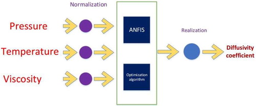
The previous works have some limitations in the accuracy of the range of their applications and also the experimental works on this issue require a considerable amount of time and cost. Due to these facts, the importance of the development of an accurate and comprehensive method that has minimum cost has been highlighted. In order to accurate estimation of carbon dioxide diffusivity in solution with various salinities, the importance of proposing a general and accurate predictive algorithm becomes highlighted. On the other hand, the wide applications of artificial intelligence approaches in different parts of engineering processes and proposing the solutions for difficult issues (Baghban et al., 2016; Baghban et al., 2017a; Baghban et al., 2017b; Baghban et al., 2017b; Chau, 2017; Chuntian & Chau, 2002; Fotovatikhah et al., 2018; Moazenzadeh et al., 2018; Taherei Ghazvinei et al., 2018; Yaseen et al., 2018), cause artificial intelligence methods can be considered as an approach for estimation of CO₂ diffusivity in different conditions. First, a collection of carbon dioxide diffusivity coefficients was gathered, then, we utilized ANFIS to build a model for the prediction of carbon dioxide diffusivity coefficients in the brine system. The predicting algorithm is optimized by the utilization of five evolutionary algorithms which are DE, ACO, GA, PSO, and BP. The ability of each developed algorithm is assessed by utilization of graphical and statistical analyses and also compared with the available correlations in the literature. In order to clarify the present work, different steps are shown in Figure 1.

Figure 1. A brief summary of present work.

2. Methodology

2.1. ANFIS

Zadeh introduced FL. The main characteristic of FL is known for the advancement of the linguistic parameters into the forms of mathematical equations. The regulations of FL include a number of if–then operators to change the quantitative parameters into qualitative. Due to a lack of accuracy in the modeling process, this approach could not satisfy scholars for prediction so the coupling FL and ANN were suggested as an efficient and accurate algorithm. The proposed tool which has potentials of FL such as MFs and if–then regulations called ANFIS. ANN is implemented to tune membership functions (Shamshirbandet al., 2019; Karkevandi-Talkhooncheh et al., 2017). Takagi- TSK as one of the FIs was applied in this study. TSK used to input and output patterns for if–then rules (Najafi-Marghmaleki et al., 2017; Nikravesh et al., 2003). Such ANFIS models have been widely used in building advanced prediction models in the relevant applications (Dehghani et al., 2019; Mosavi & Edalatifar, 2018; Mosavi et al., 2018; Rezakazemi et al., 2019).

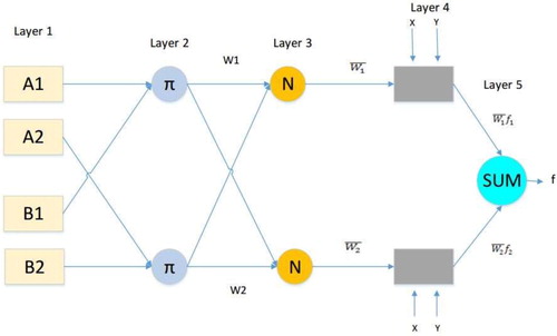
Figure 2 illustrates the structure of ANFIS network which has n input data. X_i and Y_i represent the input and output of this network. The below rules are used to construct a new model in TSK FIS:

• Rule one: IF < X₁, is A₁₁, and X₂, is A₂₁, and … and X₅, is A₅₁ > THEN < y₁ = a₁X1 + b₁X₂ + c₁X₃ + d₁X₄ + e₁X₅ + f₁>

• Rule two: IF < X₁, is A₁₂, and X₂, is A₂₂, and … and X₅, is A₅₂> THEN < y₂ = a₂X₁ + b₂X₂ + c₂X₃ + d₂X4 + e₂X₅ + f₂>

• Rule three: IF < X₁, is A₁₃, and X₂, is A₂₃, and … and X₅, is A₅₃ > THEN < y₃ = a₃X₁ + b₃X₂ + c₃X₃ + d₃X₄ + e₃X₅ + f₃>

• Rule four: IF < X₁, is A₁₄, and X₂, is A₂₄, and … and X₅, is A₅₄ > THEN < y₄ = a₄X₁ + b₄X₂ + c₄X₃ + d₄X₄ + e₄X₅ + f₄>

• Rule five: IF < X₁, is A₁₅, and X₂, is A₂₅, and … and X₅, is A₅₅ > THEN < y₅ = a₅X₁ + b₅X₂ + c₅X₃ + d₅X₄ + e₅X₅ + f₅>

• Rule fix: IF < X₁, is A₁₆, and X₂, is A₂₆, and … and X₅, is A₅₆ > THEN < y₆ = a₆X₁ + b₆X₂ + c₆X₃ + d₆X₄ + e₆X₅ + f₆>

• Rule seven: IF < X₁, is A₁₇, and X₂, is A₂₇, and … and X₅, is A₅₇ > THEN < y₇ = a₇X₁ + b₇X₂ + c₇X₃ + d₇X₄+e₇X₅+f₇>

• Rule eight: IF < X₁, is A₁₈, and X₂, is A₂₈, and … and X₅, is A₅₈ > THEN < y₈ = a₈X₁ + b₈X₂ + c₈X₃ + d₈X₄ + e₈X₅ + f₈>

Figure 2. Different layers of ANFIS algorithm.

The phrases after IF and THEN represent antecedent and consequences respectively. A and B denote the fuzzy model sets of inputs.

Figure 2 is carried out to show ANFIS model has five different layers which can be described in details as below (Dadkhah et al., 2017; Safari et al., 2014; Tatar et al., 2016):

Layer 1:

The changing of input data can be used for the creation of linguistic terms. The n nodes have been created to relate the linguistic attributes of input data. As the Gaussian functions are efficient with higher performance in prediction for algorithm so it is implemented to organize these linguistic attributes. The Gaussian functions are presented as below: (1) $O_i^1=\text{β}\left(X\right)=\text{ex}{\text{p}}^{\left(-\frac{1}{2}\frac{{\left(X-Z\right)}^2}{{\sigma }^2}\right)}$(1) Here, σ, Z and O parameters and denote to the variance, center for Gaussian MF, and output, respectively. They can be determined during the model training.

Layer 2:

The controlling of the accuracy and performance of qualifications is located in the second layer, the firing strength layer can be mentioned as another name for this layer, the following formulation explains the determination level: (2) $O_i^2=W_i={\text{β}}_{Ai}\left(X\right).{\text{β}}_{Bi}\left(X\right)$(2)

Layer 3:

The normalization of firing strength which is placed in third layer can be formulated as below: (3) $O_i^3=\frac{W_i}{{\sum }^{W_i}}$(3)

Layer 4:

The creation of linguistic terms is conducted within this layer. Furthermore, the effect of rules on outputs is presented as follow: (4) $O_i^4=\overline{W_i}{f}_i=\overline{W_i}\left(m_i{X}_1+n_i{X}_2+r_i\right)$(4) In the above expression, n_i, m_i, and r_i relate to linear parameters. In addition, the model has been developed for the purpose of reduction of the difference between the measured data and the forecasted values to optimize the parameters.

Layer 5:

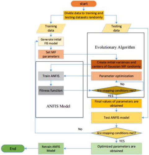
The alteration of rules to qualitative form by weighted average summation takes place in this layer as follows: (5) $O_i^5=Y=\sum _i\overline{W_i}{f}_i=\overline{W_1}{f}_1+\overline{W_2}{f}_2=\frac{{\sum }^{W_i}{f}_i}{{\sum }^{W_i}}$(5) To clarify the proposing of the algorithm, the schematic diagram of ANFIS coupled with the evolutionary algorithm is shown in Figure 3.

Figure 3. The schematic diagram of proposing predictive algorithm.

2.2. BP

BP minimizes the error by reducing the difference between estimated values and experimental data. to this end, the error is propagated back by optimization of variables in the network and biases and weights are adjusted to minimize the objective function (Afshar et al., 2014).

2.3. ACO

Dorigo introduced the ACO algorithm as an approach that is based on a population algorithm (Dorigo et al., 1996). ACO method is developed based on the natural behavior of ants to determine the shortest ways from their storage to food resources (Stützle & Hoos, 2000). Ants release a pheromone in their ways so the population can find probable paths or solutions. This approach can be applied for discrete space, not for the continuous domain. Due to this fact, a Gaussian model was proposed by the construction of a list of probable solutions to generalize this approach in continuous space. Some special solutions exist in solution archives all over time (Heris & Khaloozadeh, 2014). These solutions can be obtained by optimization algorithm.the minimization of cost function as the first step of the ACO approach starts with finding the vector $x\in X\subseteq R^{n_x}$ by the below steps (Lozano et al., 2006):

1. Initialization: generation of random N definitions in X and evaluation of cost function.

2. Solution archive: the best of the solution is described by x₁ and the worst of them is represented by x_N.

3. Weight definition: the weights for members of solution archive are determined as follows: (6) $u_i\propto \frac{1}{\sqrt{2\pi }\alpha N}\text{exp}(-\frac{1}{2}(\frac{i-1}{\alpha N}{)}^2$(6)

Based on the below condition: (7) $\sum _{i=1}^N{u}_i=1$(7)

1. Generating the probabilistic model: the Gaussian probabilistic model is constructed by the below formulations: (8) $\begin{array}{rl}{G}^j\left(X\left[j\right]\right)& =\sum _{i=1}^N{u}_{i}N\left(X\left[j\right];{\mu }_i\left[j\right];{\sigma }_i\left[j\right]\right)\end{array}$(8) (9) $\begin{array}{rl}N\left(X;\mu ;\sigma \right)& =\frac{1}{\sqrt{2\pi }\sigma }\text{exp}\left(-\frac{1}{2}{\left(\frac{x-\mu }{\sigma }\right)}^2\right)\end{array}$(9) where j and x[j] denote the decision variable and the jth part in x.

   The standard deviation and mean of Gaussian mixture are expressed in the following: (10) $\begin{array}{rl}{\mu }_i\left[j\right]& =X_i\left[j\right]\end{array}$(10) (11) $\begin{array}{rl}{\sigma }_i\left[j\right]& =\frac{\xi }{N-1}\sum _{i^{\mathrm{\prime }}=1}^N|X_i\left[j\right]-X_{i^{\mathrm{\prime }}}\left[j\right]|\end{array}$(11) where $\xi >0$ denotes the exploration/exploitation balance.

2. New samples are generated by using the model $G=\left(G^1;G^2;\dots G^{n_x}\right)$ as new members of the solution archive and their objective functions are evaluated in this part.

3. The solution for the optimization problem is chosen by selecting the best solution archive.

4. The Criterions are checked to end the optimization or restart from part 3.

2.4. DE

Differential evolution as one of the major metaheuristics methods utilizes fundamental genetic operators to investigate a population which does not require the optimization problem to be differentiable. The differential evolution method is described below (Das et al., 2011):

1. The first iteration starts as mutation factor F and crossover rate CR are selected and fitness of elements ${F_i}^k=f\left({X_i}^k\right)$ for each I are determined.

2. The mutation operator is used to generating a trial solution as below: (12) $T{X}_{i,j}=X_{a_1,j}^k+F\left(X_{a_{2}j}^k+X_{a_{3}j}^k\right)\mathrm{\forall }j\text{and}\mathrm{\forall }i$(12)

3. The crossover operator is employed on solutions as below: (13) $U_{i,j}=\left\{\begin{array}{l}T{X}_{ij}ifr\text{and}\left(\right)\le CR\text{or}j=r\text{and}b\\ X_{ij}^{k}ifr\text{and}\left(\right)>CR\text{and}j\ne r\text{and}b\end{array}\right.$(13)

   r and b represents the random index of best element b which is obtained from $r\text{and}b=r\text{and}\left(\text{D}\right)\in \{1,2,\dots ,\text{D}4$

4. Trial fitness $T{F}_i=f\left(u_{i,1},u_{i,2},\dots ,U_{i,D}\right)$ is calculated and the selection operator is applied on trial solution as below: (14) $X_{ij}^{K+1}=\left\{\begin{array}{l}{U}_{ij}\mathrm{\forall }jifT{F}_i<F_i^k\\ X_{ij}^K\mathrm{\forall }jifT{F}_i\ge F_i^k\end{array}\right.$(14)

5. Fitness estimation ${F_i}^{k+1}=f\left({X_i}^{k+1}\right)$ is done and the best index is distinguished.

6. The end criterion is checked and the explained loop restarts from part 3 if it is necessary.

2.5. GA

One of the optimization approaches which has great potential in optimizing various objective function is GA. The initial solutions of this approach which are called chromosomes are generated randomly and some actions are done on chromosomes by means of operators such as mutation, crossover, and reproduction. In this algorithm, to determine the probability of offsprings production, the CF and MF can be used (Alam et al., 2015; Bedekar & Bhide, 2011).

1. An initial solution is created randomly and CF and MF factors are generated.

2. In the second step the Chromosomes fitness, $F_i^K=f\left(X_i^k\right)$ $\mathrm{\forall }$i is determined and the best solution index $b\in \{1,$ is distinguished.

3. the various GA operators produce the new Chromosomes $X_i^{k+1},\mathrm{\forall }i$

4. the best one b1 is determined by a fitness assessment $F_i^{K+1}=f\left(X_i^{k+1}\right)$

5. In the fifth step, the old chromosome is replaced by the new best one.

6. The algorithm continues the loop to meet the best conditions.

2.6. PSO

PSO is considered as a stochastic optimization which mimics the populations in nature such as fish, birds and insects (Kennedy, 2011). In the PSO algorithm, promoting the initial populations is known as an optimization problem and particles represent the solutions (Castillo, 2012). A group of particles denotes swarm so the particle and swarm terms represent individual and population has extensive application in this algorithm and genetic algorithm(Onwunalu & Durlofsky, 2010; Sharma & Onwubolu, 2009).

In PSO algorithm, X_i(t) and V_i(t) denote position vector and velocity vector for particle i. The following equation is used for updating the particle velocity (Chen, 2013; Lin & Hong, 2007): (15) $\begin{array}{rl}{v}_{\text{id}}\left(t+1\right)& =w{v}_{\text{id}}\left(t\right)+c_1{r}_1\left(p_{\text{best,id}}\left(t\right)-X_{iid}\left(t\right)\right)\\ & +c_2{r}_2\left(g_{\text{best},d}\left(t\right)-X_{\text{id}}\left(t\right)\right),d=1,2,\dots ,D\end{array}$(15)

In Equation (16), p_best,id and g_best,id represent the best position of particle and global position r, c and w are the random number, learning rate and inertia weight. The below expression shows the next particle position (Chiou et al., 2012; Eberhart & Kennedy, 1995; Shi & Eberhart, 1998): (16) $X_{\text{id}}\left(t+1\right)=X_{\text{id}}\left(t\right)+v_{\text{id}}\left(t+1\right)d=1,2,\dots ,D$(16)

2.7. Data gathering

Efficiency and accuracy of any estimating algorithm are highly dependent on the accuracy of experimental data used for the development of the predictive model (Das et al., 2011; Hajirezaie et al., 2017; Karkevandi-Talkhooncheh et al., 2017). So we gathered 86 actual data for the carbon dioxide diffusion coefficient in the brine system from the reliable papers (S. P. Cadogan et al., 2014b; Choudhari & Doraiswamy, 1972; Maharajh, 1973; Frank et al., 1996; Himmelblau, 1964; Hirai et al., 1997; Lu et al., 2013; D. M. Maharajh & Walkley, 1973; Nijsing et al., 1959; Reddy & doraiswamy, 1967; Tamimi et al., 1994; Tan & Thorpe, 1992; Thomas & Adams, 1965; Versteeg & Van Swaaij, 1988; J. Vivian & Peaceman, 1956). The experimental data consist of diffusion coefficients of carbon dioxide in the brine system as a function of viscosity, pressure, and temperature. The collected experimental data includes the diffusion coefficients for a pressure range of 0.1–49.3 MPa, a temperature range of 273–473.15 K and a viscosity range of 0.1388–1.95 mPa.s. 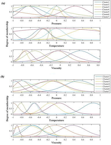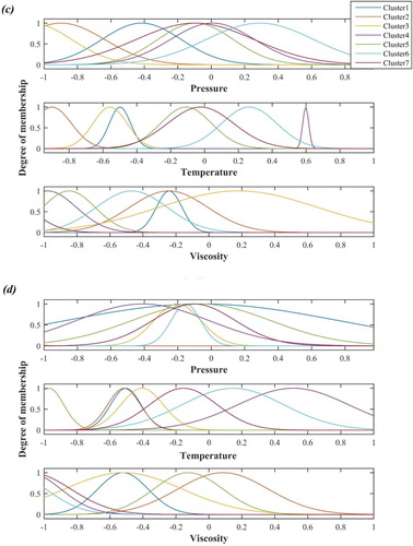In order to enhance the performance of training, the experimental data are normalized such as below: (17) $x_N=2\frac{x-x_{\text{min}}}{x_{\text{max}}-x_{\text{min}}}-1$(17) The degree of membership functions for different inputs of algorithms are shown in Figure 4.

Figure 4. Degree of membership function for (a) PSO, (b) GA, (c) ACO, (d) BP, (e) DE.

3. Results and discussion

In this paper, the ANFIS algorithm was combined with GA, ACO, PSO, DE, and BP to estimate the diffusivity coefficient in terms of temperature, pressure, and viscosity. In order to investigate the performance of the developed models, different statistical parameters such as the R², MAREs, RMSEs and STD were calculated and reported in Table 2. The aforementioned indexes were determined such as following formulations: (18) $\begin{array}{rl}{R}^2& =1-\frac{{\sum }_{i=1}^N{\left(X_i^{\text{actual}}-X_i^{\text{predicted}}\right)}^2}{{\sum }_{i=1}^N{\left(X_i^{\text{actual}}-\overline{X^{\text{actual}}}\right)}^2}\end{array}$(18) (19) $\begin{array}{rl}MARE& =\frac{1}{N}\sum _{i=1}^N\frac{|X_i^{\text{predicted}}-X_i^{\text{actual}}|}{X_i^{\text{actual}}}\end{array}$(19) (20) $\begin{array}{rl}RMSE& =\sqrt{\frac{1}{N}\sum _{i=1}^N{\left(X_i^{\text{actual}}-X_i^{\text{predicted}}\right)}^2}\end{array}$(20) (21) $\begin{array}{rl}ST{D}_{\text{error}}& ={\left(\frac{1}{N-1}\sum _{i=1}^N\left(\text{error}-\overline{\text{error}}\right)\right)}^{0.5}\end{array}$(21)

Table 2. The determined statistical parameters for proposed different algorithms.

		R^2	MARE%	RMSE	STD
PSO-ANFIS	Train	0.9993	2.0945	0.0869	0.0738
	Test	0.9978	2.7188	0.113	0.0949
GA-ANFIS	Train	0.9957	4.2591	0.2156	0.1607
	Test	0.9932	4.9245	0.1976	0.1423
ACO-ANFIS	Train	0.9924	5.9726	0.2877	0.212
	Test	0.9854	6.6933	0.3161	0.2431
BP-ANFIS	Train	0.9862	12.2787	0.3905	0.2538
	Test	0.9738	12.787	0.398	0.259
DE-ANFIS	Train	0.9708	14.545	0.633	0.462
	Test	0.9514	15.965	0.533	0.351

The determined R² values in the testing phase were 0.997753, 0.993202, 0.985409, 0.973849 and 0.951371 for ANFIS optimized by PSO, GA, ACO, BP, and DE respectively. Furthermore, RMSE values were 0.112953, 0.197641, 0.316064, 0.398 and 0.533 for them. Also for four different empirical correlations, these statistical parameters were determined and shown in Table 3. The comparisons of these parameters exhibit that the proposed ANFIS algorithm combined with an appropriate evolutionary algorithm can be better predictive machine respect to the other published correlations.

The experimental and estimated diffusion coefficients are demonstrated simultaneously in Figure 5 for different evolutionary algorithms. This comparison expresses good consistency between actual and predicted diffusivity coefficients for proposed algorithms. In order to illustrate the consistency, the experimental diffusivity is depicted against predicted diffusivity in Figure 6 for ANFIS with different evolutionary algorithms. The resulted points for total data lie near to the bisector of the first quadrant which means the high capacity and great performance of algorithms. Furthermore, the determined fitting lines have formulations near the y = x line. One of the great approaches in the graphical analysis is the depiction of relative deviations for total datasets. So the relative deviations of predicted and actual diffusivity coefficients of different algorithms are shown in Figure 7. This analysis shows the low errors in the prediction of diffusivity for ANFIS combined with different algorithms. The ranges of relative error for different optimization processes are very low and also the PSO algorithm has better performance in comparison with others.

Figure 5. The comparison of experimental and predicted diffusivity coefficient for (a) PSO, (b) GA, (c) ACO, (d) BP, (e) DE.

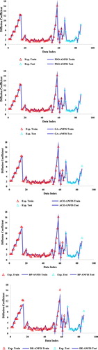
Figure 6. The experimental diffusivity coefficient versus predicted diffusivity coefficient for (a) PSO, (b) GA, (c) ACO, (d) BP, (e) DE.

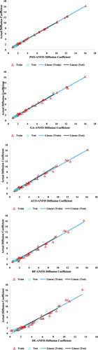
Figure 7. The relative deviation of experimental and estimated diffusivity for (a) PSO, (b) GA, (c) ACO, (d) BP, (e) DE.

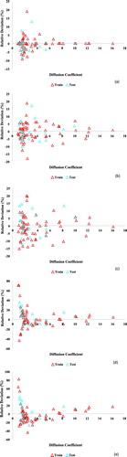
Table 3. The determined statistical indexes for the empirical correlations.

	Othmer and Thakar	Wilke and Chang	Lu et al.	Cadogan et al.
R^2	0.9566	0.9582	0.9595	0.9865
RMSE (×10^−9 m^2/s)	0.5763	0.7457	0.561	0.352
MARE (%)	8.79	7.39	10.2	8
MAE (×10^−9 m^2/s)	0.3458	0.3327	0.3453	0.2487

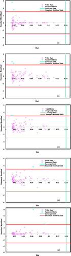
As mentioned before one of the important factors which have great impact on accuracy and performance of the model is accuracy and error of measured data points (Rousseeuw & Leroy, 2005), however the measured data utilized in the present paper were gathered from the reliable literature, due to experimental equipment and conditions they might contain some errors. Thus, here, the Leverage method has been employed to determine the inaccurate measured data. Referring to this computational method, the residuals are calculated and then inputs are utilized to organize Hat matrix by the below expression (Mohammadi et al., 2012b): (22) $H=X(X^{T}X{)}^{-1}{X}^T$(22)

In the above expression, X is known as the m×n matrix that n and m are the model parameters number and number of samples respectively. In order to the identification of inaccurate data and outliers of the dataset, William's diagram was plotted for outlier realization. As shown in Figure 8, the used data has some inaccurate and suspected data. These data are distinguished through standard residual indexes and limitations of the Leverage which are between −3 and 3. The leverage limit presented by H* can be determined by the below expression(Mohammadi et al., 2012a): (23) $H^{\ast }=3\left(n+1\right)/m$(23)

Figure 8. William's plots depicted for (a) PSO, (b) GA, (c) ACO, (d) BP, (e) DE.

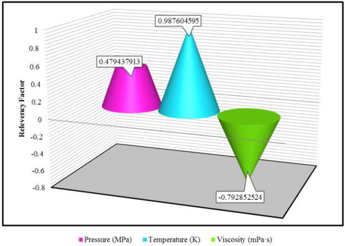
The validity and generality of the proposed model for the diffusivity coefficient of carbon dioxide prediction at different conditions are illustrated in this study. The Relevancy factor is utilized to study the impact of input variables on diffusivity. The Relevancy factor can be formulated as following (Bemani et al., 2019; Razavi et al., 2019b; Razavi et al., 2019a): (24) $r=\frac{{\sum }_{i=1}^n(X_{k,i}-\overline{X_k})\left(Y_i-\overline{Y}\right)}{\sqrt{{\sum }_{i=1}^n{(X_{k,i}-\overline{X_k})}^2{\sum }_{i=1}^n(Y_i-{\overline{Y)}}^2}}$(24) where $Y_i$,$\overline{Y}$,$X_{k,i}$ and $\overline{X_k}$ denote the ‘i’ th output, output average, kth of input, and average of input. The range of absolute value of r is lower than one and as the absolute value of r is near to one the effectiveness of the input parameter on the diffusion coefficient is higher. Figure 8 shows the Relevancy factor of the diffusivity coefficient in terms of different parameters for ANFIS combined with five different evolutionary algorithms. This analysis shows that the temperature is the most effective input parameter on the diffusivity coefficient of carbon dioxide. Furthermore, temperature and pressure have a straight relationship with the diffusivity coefficient of carbon dioxide and also it can be seen that as viscosity increases, the coefficient decreases. According to the above discussions, a present study is a helpful tool for engineers and scientists (Figure 9).

Figure 9. The calculated Relevancy factor of diffusivity coefficient in terms of different parameters.

4. Conclusions

We proposed the ANFIS coupled with five different evolutionary algorithms to estimate CO₂ diffusivity in the brine system. In order to train and test these models, a total number of 86 measured data were collected from previous works. The different statistical indicators and graphical analysis demonstrated the high efficiency and accurate ability of proposing models. The determined R² values in the testing phase were 0.9978, 0.9932, 0.9854, 0.9738 and 0.9514 for ANFIS optimized by PSO, GA, ACO, BP, and DE respectively. Also for general evaluation of model four empirical correlations from previous papers were utilized and compared with the proposed algorithms. According to the aforementioned results, it can be concluded that proposed algorithms have better performance in the prediction of carbon dioxide diffusion coefficients. Moreover, sensitivity analysis showed that temperature and pressure are the most and least effective parameters on the carbon dioxide diffusion coefficient. As a recommendation for future works, it can be suggested that other machine methods can be used for the prediction of the carbon dioxide diffusivity coefficient. However, it is worthy to mention that these methods have a limitation or drawback in comparison with experimental works which is a dependency of the accuracy of the proposed models on the accuracy and amount of databanks.

Acknowledgements

We acknowledge the “Open Access Funding by the Publication Fund of the TU Dresden”. We also acknowledge the financial support of this work by the Hungarian State and the European Union under the EFOP-3.6.1-16-2016-00010 project and the 2017-1.3.1-VKE-2017-00025 project. This research has been additionally supported by the Project: “Support of research and development activities of the J. Selye University in the field of Digital Slovakia and creative industry” of the Research and Innovation Operational Programme (ITMS code: NFP313010T504) co-funded by the European Regional Development Fund.

Disclosure statement

No potential conflict of interest was reported by the author(s).

Correction Statement

This article has been republished with minor changes. These changes do not impact the academic content of the article.

References

- Afshar, M., Gholami, A., & Asoodeh, M. (2014). Genetic optimization of neural network and fuzzy logic for oil bubble point pressure modeling. Korean Journal of Chemical Engineering, 31(3), 496–502. https://doi.org/10.1007/s11814-013-0248-8
- Agartan, E., Trevisan, L., Cihan, A., Birkholzer, J., Zhou, Q., & Illangasekare, T. H. (2015). Experimental study on effects of geologic heterogeneity in enhancing dissolution trapping of supercritical CO2. Water Resources Research, 51(3), 1635–1648. https://doi.org/10.1002/2014WR015778
- Alam, M. N., Das, B., & Pant, V. (2015). A comparative study of metaheuristic optimization approaches for directional overcurrent relays coordination. Electric Power Systems Research, 128, 39–52. https://doi.org/10.1016/j.epsr.2015.06.018
- Baghban, A., Bahadori, A., Mohammadi, A. H., & Behbahaninia, A. (2017a). Prediction of CO2 loading capacities of aqueous solutions of absorbents using different computational schemes. International Journal of Greenhouse Gas Control, 57, 143–161. https://doi.org/10.1016/j.ijggc.2016.12.010
- Baghban, A., Bahadori, M., Rozyn, J., Lee, M., Abbas, A., Bahadori, A., & Rahimali, A. (2016). Estimation of air dew point temperature using computational intelligence schemes. Applied Thermal Engineering, 93, 1043–1052. https://doi.org/10.1016/j.applthermaleng.2015.10.056
- Baghban, A., Kardani, M. N., & Habibzadeh, S. (2017b). Prediction viscosity of ionic liquids using a hybrid LSSVM and group contribution method. Journal of Molecular Liquids, 236, 452–464. https://doi.org/10.1016/j.molliq.2017.04.019
- Baghban, A., Mohammadi, A. H., & Taleghani, M. S. (2017b). Rigorous modeling of CO2 equilibrium absorption in ionic liquids. International Journal of Greenhouse Gas Control, 58, 19–41. https://doi.org/10.1016/j.ijggc.2016.12.009
- Bai, D., Zhang, X., Chen, G., & Wang, W. (2012). Replacement mechanism of methane hydrate with carbon dioxide from microsecond molecular dynamics simulations. Energy & Environmental Science, 5(5), 7033–7041. https://doi.org/10.1039/c2ee21189k
- Bedekar, P. P., & Bhide, S. R. (2011). Optimum coordination of directional overcurrent relays using the hybrid GA-NLP approach. IEEE Transactions on Power Delivery, 26(1), 109–119. https://doi.org/10.1109/TPWRD.2010.2080289
- Bemani, A., Baghban, A., & Mohammadi, A. H. (2019). An insight into the modeling of sulfur solubility of sour gases in supercritical region. Journal of Petroleum Science and Engineering, 184, 106459–106470. https://doi.org/10.1016/j.petrol.2019.106459.
- Bodnar, L., & Himmelblau, D. (1962). Continuous measurement of diffusion coefficients of gases in liquids using glass scintillators. The International Journal of Applied Radiation and Isotopes, 13(1), 1–6. https://doi.org/10.1016/0020-708X(62)90159-X
- Brignole, E., & Echarte, R. (1981). Mass transfer in laminar liquid jets: Measurement of diffusion coefficients. Chemical Engineering Science, 36(4), 705–711. https://doi.org/10.1016/0009-2509(81)85085-3
- Cadogan, S. (2015). Diffusion of CO2 in fluids relevant to carbon capture, utilisation and storage.
- Cadogan, S. P., Hallett, J. P., Maitland, G. C., & Trusler, J. M. (2014a). Diffusion coefficients of carbon dioxide in brines measured using 13C pulsed-field gradient nuclear magnetic resonance. Journal of Chemical & Engineering Data, 60(1), 181–184. https://doi.org/10.1021/je5009203
- Cadogan, S. P., Maitland, G. C., & Trusler, J. M. (2014b). Diffusion coefficients of CO2 and N2 in water at temperatures between 298.15 and 423.15 K at pressures up to 45 MPa. Journal of Chemical & Engineering Data, 59(2), 519–525. https://doi.org/10.1021/je401008s
- Castillo, O. (2012). Introduction to type-2 fuzzy logic control Type-2 fuzzy logic in intelligent control applications (pp. 3-5). Springer.
- Chang, F., Jin, J., Zhang, N., Wang, G., & Yang, H.-J. (2012). The effect of the end group, molecular weight and size on the solubility of compounds in supercritical carbon dioxide. Fluid Phase Equilibria, 317, 36–42. https://doi.org/10.1016/j.fluid.2011.12.018
- Chau, K.-W. (2017). Use of meta-heuristic techniques in rainfall-runoff modelling. MDPI. doi:10.3390/w9030186.
- Chen, M.-Y. (2013). A hybrid ANFIS model for business failure prediction utilizing particle swarm optimization and subtractive clustering. Information Sciences, 220, 180–195. https://doi.org/10.1016/j.ins.2011.09.013
- Chiou, J.-S., Tsai, S.-H., & Liu, M.-T. (2012). A PSO-based adaptive fuzzy PID-controllers. Simulation Modelling Practice and Theory, 26, 49–59. https://doi.org/10.1016/j.simpat.2012.04.001
- Choudhari, R., & Doraiswamy, L. (1972). Physical properties in reaction of ethylene and hydrogen chloride in liquid media. Diffusivities and solubilities. Journal of Chemical and Engineering Data, 17(4), 428–432. https://doi.org/10.1021/je60055a012
- Chuntian, C., & Chau, K.-W. (2002). Three-person multi-objective conflict decision in reservoir flood control. European Journal of Operational Research, 142(3), 625–631. https://doi.org/10.1016/S0377-2217(01)00319-8
- Cui, G., Zhang, L., Ren, B., Enechukwu, C., Liu, Y., & Ren, S. (2016). Geothermal exploitation from depleted high temperature gas reservoirs via recycling supercritical CO2: Heat mining rate and salt precipitation effects. Applied Energy, 183, 837–852. https://doi.org/10.1016/j.apenergy.2016.09.029
- Dadkhah, M. R., Tatar, A., Mohebbi, A., Barati-Harooni, A., Najafi-Marghmaleki, A., Ghiasi, M. M., Mohammadi A. H., & Pourfayaz, F. (2017). Prediction of solubility of solid compounds in supercritical CO2 using a connectionist smart technique. The Journal of Supercritical Fluids, 120, 181–190. https://doi.org/10.1016/j.supflu.2016.06.006
- Das, S., Mukhopadhyay, A., Roy, A., Abraham, A., & Panigrahi, B. K. (2011). Exploratory power of the harmony search algorithm: Analysis and improvements for global numerical optimization. IEEE Transactions on Systems, Man, and Cybernetics, Part B (Cybernetics), 41(1), pp. 89-106. https://doi.org/10.1109/TSMCB.2010.2046035
- Dehghani, M., Riahi-Madvar, H., Hooshyaripor, F., Mosavi, A., Shamshirband, S., Zavadskas, E. K., & Chau, K.-W. (2019). Prediction of Hydropower Generation using Grey Wolf optimization adaptive neuro-fuzzy inference system. Energies, 12(2), 289. https://doi.org/10.3390/en12020289
- Dorigo, M., Maniezzo, V., & Colorni, A. (1996). Ant system: Optimization by a colony of cooperating agents. IEEE Transactions on Systems, Man, and Cybernetics, Part B (Cybernetics), 26(1), 29–41. https://doi.org/10.1109/3477.484436
- Eberhart, R., & Kennedy, J. (1995). A new optimizer using particle swarm theory. Micro machine and Human Science, 1995. MHS’95.10-14 June. Proceedings of the Sixth International Symposium on.
- Eccles, J. K., Pratson, L., Newell, R. G., & Jackson, R. B. (2009). Physical and economic potential of geological CO2 storage in saline aquifers. Environmental Science & Technology, 43(6), 1962–1969. https://doi.org/10.1021/es801572e
- Farajzadeh, R., Zitha, P. L., & Bruining, J. (2009). Enhanced mass transfer of CO2 into water: Experiment and modeling. Industrial & Engineering Chemistry Research, 48(13), 6423–6431. https://doi.org/10.1021/ie801521u
- Fotovatikhah, F., Herrera, M., Shamshirband, S., Chau, K.-W., Faizollahzadeh Ardabili, S., & Piran, M. J. (2018). Survey of computational intelligence as basis to big flood management: Challenges, research directions and future work. Engineering Applications of Computational Fluid Mechanics, 12(1), 411–437. https://doi.org/10.1080/19942060.2018.1448896
- Frank, M. J., Kuipers, J. A., & van Swaaij, W. P. (1996). Diffusion coefficients and viscosities of CO2+ H2O, CO2+ CH3OH, NH3+ H2O, and NH3+ CH3OH liquid mixtures. Journal of Chemical & Engineering Data, 41(2), 297–302. https://doi.org/10.1021/je950157k
- Guzmán, J., & Garrido, L. (2012). Determination of carbon dioxide transport coefficients in liquids and polymers by NMR spectroscopy. The Journal of Physical Chemistry B, 116(20), 6050–6058. https://doi.org/10.1021/jp302037w
- Hajirezaie, S., Pajouhandeh, A., Hemmati-Sarapardeh, A., Pournik, M., & Dabir, B. (2017). Development of a robust model for prediction of under-saturated reservoir oil viscosity. Journal of Molecular Liquids, 229, 89–97. https://doi.org/10.1016/j.molliq.2016.11.088
- Hemmati-Sarapardeh, A., Ayatollahi, S., Ghazanfari, M.-H., & Masihi, M. (2013). Experimental determination of interfacial tension and miscibility of the CO2–crude oil system; temperature, pressure, and composition effects. Journal of Chemical & Engineering Data, 59(1), 61–69. https://doi.org/10.1021/je400811h
- Heris, S. M. K., & Khaloozadeh, H. (2014). Ant colony estimator: An intelligent particle filter based on ACOR. Engineering Applications of Artificial Intelligence, 28, 78–85. https://doi.org/10.1016/j.engappai.2013.11.005
- Himmelblau, D. (1964). Diffusion of dissolved gases in liquids. Chemical Reviews, 64(5), 527–550. https://doi.org/10.1021/cr60231a002
- Hirai, S., Okazaki, K., Yazawa, H., Ito, H., Tabe, Y., & Hijikata, K. (1997). Measurement of CO2 diffusion coefficient and application of LIF in pressurized water. Energy, 22(2-3), 363–367. https://doi.org/10.1016/S0360-5442(96)00135-1
- Jähne, B., Heinz, G., & Dietrich, W. (1987). Measurement of the diffusion coefficients of sparingly soluble gases in water. Journal of Geophysical Research: Oceans, 92(C10), 10767–10776. https://doi.org/10.1029/JC092iC10p10767
- Javadpour, F. (2009). CO2 injection in geological formations: Determining macroscale coefficients from pore scale processes. Transport in Porous Media, 79(1), 87. https://doi.org/10.1007/s11242-008-9289-6
- Karkevandi-Talkhooncheh, A., Hajirezaie, S., Hemmati-Sarapardeh, A., Husein, M. M., Karan, K., & Sharifi, M. (2017). Application of adaptive neuro fuzzy interface system optimized with evolutionary algorithms for modeling CO2-crude oil minimum miscibility pressure. Fuel, 205, 34–45. https://doi.org/10.1016/j.fuel.2017.05.026
- Kennedy, J. (2011). Particle swarm optimization Encyclopedia of machine learning (pp. 760–766). Springer.
- Li, Z., & Gu, Y. (2014). Optimum timing for miscible CO2-EOR after waterflooding in a tight sandstone formation. Energy & Fuels, 28(1), 488–499. https://doi.org/10.1021/ef402003r
- Liger-Belair, G., Prost, E., Parmentier, M., Jeandet, P., & Nuzillard, J.-M. (2003). Diffusion coefficient of CO2 molecules as determined by 13C NMR in various carbonated beverages. Journal of Agricultural and Food Chemistry, 51(26), 7560–7563. https://doi.org/10.1021/jf034693p
- Lin, C.-J., & Hong, S.-J. (2007). The design of neuro-fuzzy networks using particle swarm optimization and recursive singular value decomposition. Neurocomputing, 71(1-3), 297–310. https://doi.org/10.1016/j.neucom.2006.12.016
- Lozano, J. A., Larrañaga, P., Inza, I., & Bengoetxea, E. (2006). Towards a new evolutionary computation: Advances on estimation of distribution algorithms. Springer.
- Lu, W., Guo, H., Chou, I.-M., Burruss, R., & Li, L. (2013). Determination of diffusion coefficients of carbon dioxide in water between 268 and 473 K in a high-pressure capillary optical cell with in situ Raman spectroscopic measurements. Geochimica et Cosmochimica Acta, 115, 183–204. https://doi.org/10.1016/j.gca.2013.04.010
- Maharajh, D. (1973). Solubility and diffusion of gases in water (Simon Fraser University. Theses (Dept. of Chemistry).
- Maharajh, D. M., & Walkley, J. (1973). The temperature dependence of the diffusion coefficients of Ar, CO2, CH4, CH3Cl, CH3Br, and CHCl2F in water. Canadian Journal of Chemistry, 51(6), 944–952. https://doi.org/10.1139/v73-140
- Mazarei, A. F., & Sandall, O. C. (1980). Diffusion coefficients for helium, hydrogen, and carbon dioxide in water at 25 C. AIChE Journal, 26(1), 154–157. https://doi.org/10.1002/aic.690260128
- Moazenzadeh, R., Mohammadi, B., Shamshirband, S., & Chau, K.-W. (2018). Coupling a firefly algorithm with support vector regression to predict evaporation in northern Iran. Engineering Applications of Computational Fluid Mechanics, 12(1), 584–597. https://doi.org/10.1080/19942060.2018.1482476
- Mohammadi, A. H., Eslamimanesh, A., Gharagheizi, F., & Richon, D. (2012a). A novel method for evaluation of asphaltene precipitation titration data. Chemical Engineering Science, 78, 181–185. https://doi.org/10.1016/j.ces.2012.05.009
- Mohammadi, A. H., Gharagheizi, F., Eslamimanesh, A., & Richon, D. (2012b). Evaluation of experimental data for wax and diamondoids solubility in gaseous systems. Chemical Engineering Science, 81, 1–7. https://doi.org/10.1016/j.ces.2012.06.051
- Mosavi, A., & Edalatifar, M. (2018). A Hybrid neuro-fuzzy algorithm for prediction of Reference Evapotranspiration. International Conference on global Research and Education, Kaunas, Lithuania, 24-27 September.
- Mosavi, A., Ozturk, P., & Chau, K.-W. (2018). Flood prediction using machine learning models: Literature review. Water, 10(11), 1536. https://doi.org/10.3390/w10111536
- Moultos, O. A., Tsimpanogiannis, I. N., Panagiotopoulos, A. Z., & Economou, I. G. (2016). Self-diffusion coefficients of the binary (H2O+ CO2) mixture at high temperatures and pressures. The Journal of Chemical Thermodynamics, 93, 424–429. https://doi.org/10.1016/j.jct.2015.04.007
- Mutoru, J. W., Leahy-Dios, A., & Firoozabadi, A. (2011). Modeling infinite dilution and Fickian diffusion coefficients of carbon dioxide in water. AIChE Journal, 57(6), 1617–1627. https://doi.org/10.1002/aic.12361
- Najafi-Marghmaleki, A., Barati-Harooni, A., Tatar, A., Mohebbi, A., & Mohammadi, A. H. (2017). On the prediction of Watson characterization factor of hydrocarbons. Journal of Molecular Liquids, 231, 419–429. https://doi.org/10.1016/j.molliq.2017.01.098
- Ng, W. Y., & Walkley, J. (1969). Diffusion of gases in liquids: The constant size bubble method. Canadian Journal of Chemistry, 47(6), 1075–1077. https://doi.org/10.1139/v69-170
- Nijsing, R., Hendriksz, R., & Kramers, H. (1959). Absorption of CO2 in jets and falling films of electrolyte solutions, with and without chemical reaction. Chemical Engineering Science, 10(1-2), 88–104. https://doi.org/10.1016/0009-2509(59)80028-2
- Nikravesh, M., Zadeh, L. A., & Aminzadeh, F. (2003). Soft computing and intelligent data analysis in oil exploration. Elsevier.
- Onwunalu, J. E., & Durlofsky, L. J. (2010). Application of a particle swarm optimization algorithm for determining optimum well location and type. Computational Geosciences, 14(1), 183–198. https://doi.org/10.1007/s10596-009-9142-1
- Ota, M., Saito, T., Aida, T., Watanabe, M., Sato, Y., Smith, R. L., & Inomata, H. (2007). Macro and microscopic CH4–CO2 replacement in CH4 hydrate under pressurized CO2. AIChE Journal, 53(10), 2715–2721. https://doi.org/10.1002/aic.11294
- Othmer, D. F., & Thakar, M. S. (1953). Correlating diffusion coefficient in liquids. Industrial & Engineering Chemistry, 45(3), 589–593. https://doi.org/10.1021/ie50519a036
- Pratt, K., Slater, D., & Wakeham, W. (1973). A rapid method for the determination of diffusion coefficients of gases in liquids. Chemical Engineering Science, 28(10), 1901–1903. https://doi.org/10.1016/0009-2509(73)85074-2
- Pruess, K. (2006). Enhanced geothermal systems (EGS) using CO2 as working fluid—A novel approach for generating renewable energy with simultaneous sequestration of carbon. Geothermics, 35(4), 351–367. https://doi.org/10.1016/j.geothermics.2006.08.002
- Rau, G. H., & Caldeira, K. (1999). Enhanced carbonate dissolution:: A means of sequestering waste CO2 as ocean bicarbonate. Energy Conversion and Management, 40(17), 1803–1813. https://doi.org/10.1016/S0196-8904(99)00071-0
- Razavi, R., Bemani, A., Baghban, A., Mohammadi, A. H., & Habibzadeh, S. (2019a). An insight into the estimation of fatty acid methyl ester based biodiesel properties using a LSSVM model. Fuel, 243, 133–141. https://doi.org/10.1016/j.fuel.2019.01.077
- Razavi, R., Sabaghmoghadam, A., Bemani, A., Baghban, A., Chau, K.-W., & Salwana, E. (2019b). Application of anfis and lssvm strategies for estimating thermal conductivity enhancement of metal and metal oxide based nanofluids. Engineering Applications of Computational Fluid Mechanics, 13(1), 560–578. https://doi.org/10.1080/19942060.2019.1620130
- Reddy, k., & doraiswamy, l. (1967). Estimating liquid diffusivity. Industrial & Engineering Chemistry Fundamentals, 6(1), 77–79. https://doi.org/10.1021/i160021a012
- Ren, B., Sun, Y., & Bryant, S. (2014). Maximizing local capillary trapping during CO2 injection. Energy Procedia, 63, 5562–5576. https://doi.org/10.1016/j.egypro.2014.11.590
- Ren, B., Zhang, L., Huang, H., Ren, S., Chen, G., & Zhang, H. (2015). Performance evaluation and mechanisms study of near-miscible CO2 flooding in a tight oil reservoir of Jilin Oilfield China. Journal of Natural Gas Science and Engineering, 27, 1796–1805. https://doi.org/10.1016/j.jngse.2015.11.005
- Rezakazemi, M., Mosavi, A., & Shirazian, S. (2019). ANFIS pattern for molecular membranes separation optimization. Journal of Molecular Liquids, 274, 470–476. https://doi.org/10.1016/j.molliq.2018.11.017
- Rousseeuw, P. J., & Leroy, A. M. (2005). Robust regression and outlier detection. John wiley & sons.
- Safari, H., Nekoeian, S., Shirdel, M. R., Ahmadi, H., Bahadori, A., & Zendehboudi, S. (2014). Assessing the dynamic viscosity of Na–K–Ca–Cl–H2O aqueous solutions at high-pressure and high-temperature conditions. Industrial & Engineering Chemistry Research, 53(28), 11488–11500. https://doi.org/10.1021/ie501702z
- Shamshirband, S., Hadipoor, M., & Baghban, A. (2019). Developing an ANFIS-PSO Model to Predict Mercury Emissions in Combustion Flue Gases. Mathematics, 7, 965–985. DOI:10.3390/math7100965.
- Sharma, A., & Onwubolu, G. (2009). Hybrid particle swarm optimization and GMDH system Hybrid Self-Organizing modeling systems (pp. 193–231). Springer.
- Shi, Y., & Eberhart, R. (1998). A modified particle swarm optimizer. Evolutionary Computation Proceedings, 1998. IEEE World Congress on Computational intelligence.8-12 August. The 1998 IEEE International Conference on.
- Stützle, T., & Hoos, H. H. (2000). MAX–MIN ant system. Future Generation Computer Systems, 16(8), 889–914. https://doi.org/10.1016/S0167-739X(00)00043-1
- Taherei Ghazvinei, P., Hassanpour Darvishi, H., Mosavi, A., Yusof, K., Alizamir, M., Shamshirband, S., & & Chau, K.-W. (2018). Sugarcane growth prediction based on meteorological parameters using extreme learning machine and artificial neural network. Engineering Applications of Computational Fluid Mechanics, 12(1), 738–749. https://doi.org/10.1080/19942060.2018.1526119
- Tamimi, A., Rinker, E. B., & Sandall, O. C. (1994). Diffusion coefficients for hydrogen sulfide, carbon dioxide, and nitrous oxide in water over the temperature range 293-368 K. Journal of Chemical and Engineering Data, 39(2), 330–332. https://doi.org/10.1021/je00014a031
- Tan, K., & Thorpe, R. (1992). Gas diffusion into viscous and non-Newtonian liquids. Chemical Engineering Science, 47(13-14), 3565–3572. https://doi.org/10.1016/0009-2509(92)85071-I
- Tatar, A., Barati-Harooni, A., Najafi-Marghmaleki, A., Norouzi-Farimani, B., & Mohammadi, A. H. (2016). Predictive model based on ANFIS for estimation of thermal conductivity of carbon dioxide. Journal of Molecular Liquids, 224, 1266–1274. https://doi.org/10.1016/j.molliq.2016.10.112
- Tham, M., Bhatia, K., & Gubbins, K. (1967). Steady-state method for studying diffusion of gases in liquids. Chemical Engineering Science, 22(3), 309–311. https://doi.org/10.1016/0009-2509(67)80117-9
- Thomas, W., & Adams, M. (1965). Measurement of the diffusion coefficients of carbon dioxide and nitrous oxide in water and aqueous solutions of glycerol. Transactions of the Faraday Society, 61, 668–673. https://doi.org/10.1039/tf9656100668
- Trevisan, L., Cihan, A., Fagerlund, F., Agartan, E., Mori, H., Birkholzer, J. T., Quanlin Z., & Illangasekare, T. H. (2014a). Investigation of mechanisms of supercritical CO 2 trapping in deep saline reservoirs using surrogate fluids at ambient laboratory conditions. International Journal of Greenhouse Gas Control, 29, 35–49. https://doi.org/10.1016/j.ijggc.2014.07.012
- Trevisan, L., Pini, R., Cihan, A., Birkholzer, J. T., Zhou, Q., & Illangasekare, T. H. (2014b). Experimental investigation of supercritical CO2 trapping mechanisms at the intermediate laboratory scale in well-defined heterogeneous porous media. Energy Procedia, 63, 5646–5653. https://doi.org/10.1016/j.egypro.2014.11.597
- Versteeg, G. F., & Van Swaaij, W. P. (1988). Solubility and diffusivity of acid gases (carbon dioxide, nitrous oxide) in aqueous alkanolamine solutions. Journal of Chemical & Engineering Data, 33(1), 29–34. https://doi.org/10.1021/je00051a011
- Vivian, J. E., & King, C. J. (1964). Diffusivities of slightly soluble gases in water. AIChE Journal, 10(2), 220–221. https://doi.org/10.1002/aic.690100217
- Vivian, J., & Peaceman, D. (1956). Liquid-side resistance in gas absorption. AIChE Journal, 2(4), 437–443. https://doi.org/10.1002/aic.690020404
- Wilke, C., & Chang, P. (1955). Correlation of diffusion coefficients in dilute solutions. AIChE Journal, 1(2), 264–270. https://doi.org/10.1002/aic.690010222
- Yaseen, Z. M., Sulaiman, S. O., Deo, R. C., & Chau, K.-W. (2018). An enhanced extreme learning machine model for river flow forecasting: State-of-the-art, practical applications in water resource engineering area and future research direction. Journal of Hydrology, 569. doi:10.1016/j.jhydrol.2018.11.069.
- Zhang, L., Cui, G., Zhang, Y., Ren, B., Ren, S., & Wang, X. (2016). Influence of pore water on the heat mining performance of supercritical CO2 injected for geothermal development. Journal of CO2 Utilization, 16, 287–300. https://doi.org/10.1016/j.jcou.2016.08.008