Numerical simulation of the aerodynamic characteristics of double unit train

ABSTRACT

Double unit trains running at high speeds may create additional aerodynamic challenges due to two streamlined structures with close proximity, exploring the aerodynamic performance of double unit trains is now critical. In this study, detached eddy simulation (DES) approach was employed to study the aerodynamic performance and the nearby flow patterns of a double unit train, whose results were compared and analyzed with that of a single-unit train with a same length. The results showed that the coupling method could change the aerodynamic drag on each car and tended to increase the overall drag of the double unit train. The lift force of the front car near the coupler was significantly increased. Similar slipstream distributions were found around the front half single and double-unit train except in a region close to the coupler. Due to the coupling structure, the slipstream of the rear half of double unit train was much stronger compared to single unit train. The vortex region behind the double-unit train was much wider than that of the single-unit train and was accompanied by greater vortex-shedding.

KEYWORDS:

• Aerodynamic force
• double-unit train
• drag component
• numerical simulation
• detached eddy simulation (DES)
• open air

1. Introduction

Because of their high efficiencies and protection, high-speed railways have developed as an significant way of transport and are receiving growing attention in the world. However, as the train speeds continue to increase due to new technology, the aerodynamic performances of the trains have changed more significantly than the train speeds. Aerodynamic drag constitutes 85% of the overall resistance for a train running faster than 300 km/h, and this percentage is more than 80% for a container train operating at 115 km/h (Li et al., 2017). Excessive resistance not only leads to higher-energy consumption, but also increases the requirements on the train traction system, both of which limit the further development of high-speed trains. Reduction of a train’s aerodynamic drag would lead to fuel consumption savings, which can help save energy and reduce emissions (Akbarian et al., 2018).

Like other bodies with high length-to-width ratios (Ghalandari et al., 2019; Mou et al., 2017), high-speed trains have more complex aerodynamic characteristics than other vehicles (Chen et al., 2016; Deng et al., 2019, 2020; Hemida & Krajnović, 2010; Li et al., 2019; Niu et al., 2020). To reduce the aerodynamic drag on a train, numerous tests and simulations were carried out to investigate aerodynamic performances of various types of trains. It was found that the geometric shape and the different components of the train have significant effects on the aerodynamic drag. Shape optimization is an active field for reducing drag, and recently many researchers have conducted studies in this field (Li et al., 2016). In addition, the train formations have great impact on its aerodynamic performance. Mao et al. (2012) investigated the impact of the train length and found that it played an important role on the aerodynamic drag of the tail car, wherever it was not a monotonous relationship.

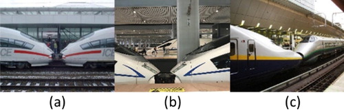
To increase the carrying capacity of railway transports, double-unit trains are often used, especially at rush hour. The proximity of these trains creates a special marshalling form in which the first tail car is coupled with the second head car, and thus, a gap appears in the middle of the train, as shown in Figure 1. Although this arrangement is commonly used, its effect on train aerodynamics has been rarely considered. Liu et al. (2019) investigated the influence of the train length and pressure propagation as well as the effects of the coupling structure on the train surface pressure and tunnel wall when a train operates in a tunnel. Niu et al. (2017) conducted simulations involving a running double-unit train and passing one another in a tunnel. However, the effect of this arrangement on the aerodynamic performance in the open air has been rarely studied in depth. Few experiments and simulations have been carried out to study the aerodynamic performance and slipstreams generated by double-unit trains (Baker et al., 2013a, 2013b; Guo et al., 2018). The focus of these studies was the effect of the coupling on the slipstream, but no attempt was made to study the aerodynamic forces. Therefore, the aim of this work is to investigate the effect double-unit trains on the aerodynamic forces with special emphasis on the drag force. A 1/20th scaled model of the Chinese high-speed train was employed in this study. Using the detached eddy simulation (DES) approach, flows were obtained around single- and double-unit trains, and the results were validated using wind tunnel tests.

Figure 1. Double unit train in different countries: (a) Germany, (b) China, and (c) Japan.

2. Methodology

2.1. Models

The shape of a popular high-speed train in China CRH2 is employed for this study. Two train models are constructed according to the research needs. Their total length is kept consistent to ensure that their aerodynamic differences are only resulted from the connecting way of the train. In this case, the whole train consists of six cars, as shown in Figure 2, the single-unit train consists of a head car, a tail car and four identical intermediate cars between them. The double-unit train can be regarded as a combination of two trains. Key parts that affect aerodynamics such as bogies and inter-car gaps are restored in the calculation model. For convenience of representation, the single- and double-unit trains are hereinafter denoted as “SUT” and “DUT,” respectively.

Figure 2. Train models employed in the numerical simulations.

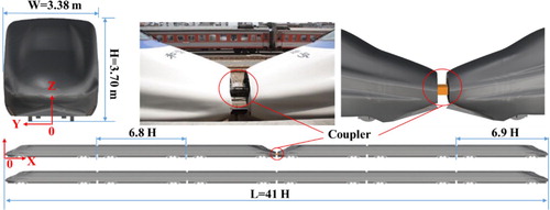
To have a dimensionless unit, the height of train models H was denoted as the characteristic dimension. Other important length parameters are shown in Figure 2.

2.2. Numerical methodology

As an efficient way to model the surrounding flow of a train (Hemida et al., 2012; Krajnović et al., 2012; Niu et al., 2020a), Large eddy simulation (LES) used in train aerodynamics are computationally costly. Reynolds Average Navier-Stokes (RANS) approach is not good to represent the real-flow characteristics around trains but much cheaper and faster. DES is the combination of LES and RANS. The time-dependent flow away from the wall boundaries is captured by LES and the mean boundary layer behavior in the area close to wall is approximated by RANS (Guo et al., 2020a). DES was commonly used in the existing previous research to simulate the turbulent flow around the trains. (Flynn et al., 2014; Guo et al., 2019; Guo et al., 2020b; Li et al., 2018, 2020; Muld et al., 2013; Niu et al., 2020b; Zhang et al., 2016).

The DES equations are based on a realizable k-ε double equation model and this work is solved in the FLUENT based on the finite volume method and a pressure-based solver. The near-wall flow is treated by the standard wall function. The time step was Δt = 5 × 10⁻⁵ s. The residual of each equation reached 10⁻⁶ in each time step. In simulations, the Reynolds number of this simulations was about 7.56 × 10⁵ according to the height of the train (H) and the train speed (60 m/s), meeting the requirement for Reynolds number in CEN (2011) standard, 2.5 × 10⁵. The value of the time-averaged results was sampled within 0.8 s.

2.3. Computational domain and boundary conditions

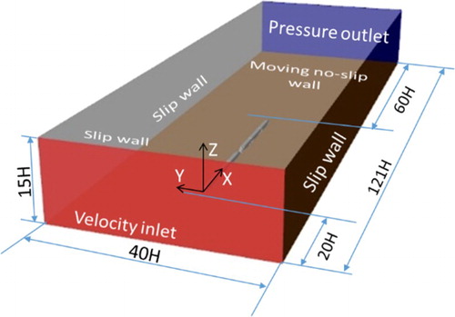
As shown in Figure 3, the upstream distance before the train nose was 20 H, the downstream distance from the outlet surface to the nose of tail car was 60 H. The domain had a width of 40 H and the train model was mounted centrally of width direction. The height of the domain was 15 H and a gap at 0.05 H was set between the wheels and the ground. A steady and uniform velocity inlet was adopted at the inlet boundary, where a speed numerically equal but opposite to the direction of the train was imposed. A zero-pressure condition was used for the outlet of the computational domain to represent the open-air condition. Slip wall conditions were used at the sides and roof to avoid the impact on the train model brought by these surfaces, who do not exist in the reality. A moving no-slip wall with a velocity equal to that of the train speed was used at the lower face of the computational domain to consider the relative motion of train to ground.

Figure 3. Computational domain, coordinate system, and boundary conditions.

2.4. Computational mesh

In this study, the meshing module included in OpenFOAM named SnappyHexMesh, was used to create unstructured hexahedral grids. To judge whether solutions were a function of the grid density or not, a grid-dependency study was conducted, in which three different meshes were used; coarse, medium, and fine meshes, consisting of 16, 25, and 37 million cells, respectively. Table 1 shows their details. Figure 4 shows the fine mesh around the train model, where an averaged y+ value of 42 was obtained.

Figure 4. Fine mesh employed in the simulations: (a) mesh density in the computational domain, (b) cell layers around head car, (c) mesh distribution around the head car, and (d) mesh distribution in the coupling region.

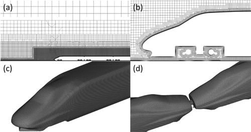
Table 1. Parameters of the three mesh configurations for the DUT model.

Items	Coarse	Medium	Fine
Total number of cells	15,945,364	25,368,422	36,845,448
The smallest cell size on train surface (mm)	4.6	2.3–4.6	2.3
Number of extra refined regions	2	2	3
Number of prism layers	6	8	10
Thickness of the first cell near the surface (mm)	0.77	0.29–0.58	0.23
Averaged dimensionless wall distance value (y^+)	140	73	42

The pressure coefficient, $c_p$ was employed to compare the results obtained by different meshes. Here, $c_p$ is defined as: (1) $c_p=\frac{P-P_0}{0.5\rho {u_{in}}^2}$(1) where $P_0$ denotes the reference pressure, $P$ is the absolute pressure, $\rho$ is air density at 20°C, and $u_{in}$ is the inlet velocity. Figure 5 shows the pressure coefficient obtained from the three meshes along curve 1, which denotes the surface curve of the head car nose along the symmetrical plane and is colored red in Figure 5.

Figure 5. Pressure distributions obtained using different meshes.

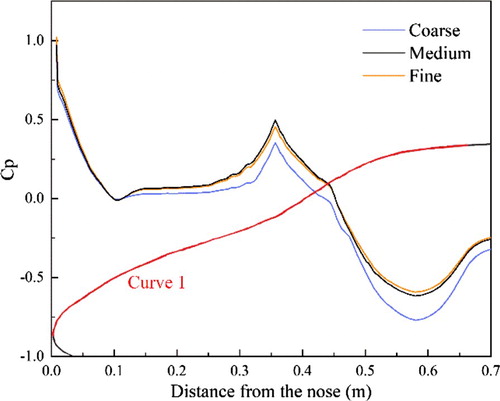
As illustrated in Figure 5, the medium mesh produced results similar with those of the fine mesh. Because only two simulations were calculated and compared in this study, which had been involved in the grid independence verification, the fine mesh configuration was used for the SUT and DUT.

3. Results

3.1. Verification

Wind tunnel test was carried out at the $8\text{m}\times 6\text{m}$ wind tunnel belonging to the China Aerodynamic Research and Development Center (Figure 6(a)). Based on the size of the cross section of wind tunnel, the three-car train model was set as a 1/8 scaling with a cross-sectional area of 0.175 m², the blockage ratio was far less than 5%. The same-scaled ballast with a rail model was installed on a rotatable disk. The force balance, piezometer, and pressure scan valve were placed in the hollow train model. Three force balances were used to capture the forces of each car. The measurement data were captured and stored by a VXI multi-channel recording system. A three-car train model was simulated to assess the reliability of numerical results (Figure 6(b)). The Reynolds numbers in the experiments and simulations were approximately 1.89 × 10⁶.

Figure 6. Wind tunnel tests and validation of simulation: (a) The train model used in the wind tunnel and (b) the simulation model with the same domain.

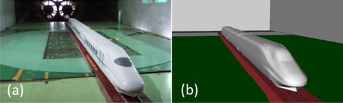
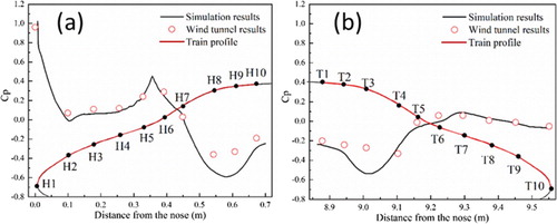
Figure 7 shows the value of $c_p$ obtained by fine mesh with DES and experiment on the symmetric plane of the train noses. These curves are colored red and the points are colored black corresponding to the red curve, which is the train profile. These points were also studied in Zhang et al. (2018). As shown in Figure 7, there was a good agreement between the simulations and experimental data. However, there were some discrepancies at points H9 and T3. These discrepancies could be related to the incomplete consistency in this transition area between the CFD models and the physical model.

Figure 7. Pressure coefficient obtained by the wind tunnel tests and simulations at: (a) symmetric line of the head nose and (b) symmetric line of the tail nose.

The values of the drag coefficient, $c_d$, obtained by fine mesh with DES and experiment are listed in Table 2. $c_d$ was defined as: (2) $c_d=\frac{D}{0.5\rho {u_{in}}^{2}A}$(2) where $D$ denotes the aerodynamic drag of the individual cars and $A$ is the cross-sectional area of the train model (11.29 m²). The discrepancy between the DES and experimental values of $c_d$ of each car was not more than 5%. This discrepancy occurred because of the irregularity of the physical model surface and some machining errors which lead to some inevitable small differences. These geometrical differences can modify the flow around the individual cars and thereby the surface pressure, as stated by Sicot et al. (2018). In addition, the turbulence of the inlet was difficult to control to achieve a similar turbulence to that in the wind tunnel, which could lead to some discrepancies in the drag coefficient. However, the difference between experimental data and the numerical results was less than 5% and this was deemed to be adequate to believe that numerical results can capture the flow features analyzed below.

Table 2. Comparison of the drag coefficient obtained from DES and the wind tunnel tests.

$c_d$ of head car			$c_d$ of intermediate car			$c_d$ of tail car
Test	Simulation	Error	Test	Simulation	Error	Test	Simulation	Error
0.147	0.140	4.8%	0.081	0.084	4.9%	0.162	0.160	1.2%

3.2. Aerodynamic drag

A train’s aerodynamic drag is contributed by the viscous resistance and pressure resistance. These two forces are likely to be generated quite differently on each section of the train, which results in various aerodynamic performances of the aerodynamic drag on each car.

Figure 8 shows the aerodynamic drag coefficient acting on each car of single- and double-unit train with the contributions of the pressure and viscous resistances in the total drag. The drag coefficients of the first and the last intermediate car (i.e. the second and the fifth car for the whole train) of the SUT were relatively higher than those of the other intermediate cars. This was due to the flow separation around the head and tail car that produced different flow fields around these two cars, which resulted in different surface pressures and boundary layers. The lowest $c_d$ for the SUT appeared to be on the second and third intermediate cars (i.e. the third and the fourth car for the whole train), which were attributed to the relatively stable flow around these two cars, and the air friction resistance dominated. Total drag of the head car of DUT and SUT was the same. This was expected, as they were exposed to the same flow conditions and were far from the coupler position. Some of the differences in the surrounding flow field, influenced by the downstream fake tail car (the third car of DUT), were present on the second car, causing a smaller differential pressure drag to be distributed on this car, the drag of the second car of DUT was lower. Like a tail car, the airflow converged under the guidance of the streamlined structure, a large positive pressure was supposed to form on the nose region, which was removed and linked by a coupler. This car therefore lost a huge contribution to the aerodynamic drag, and its $c_d$ was even lower than the second intermediate car of the SUT. The fourth car suffered from significant flow separation again, and thus, it had the largest drag among the cars. After a transition by the fourth car, the turbulence intensity of the surrounding flow was weakened around the fifth car, while it is plausible that its drag was still larger.

Figure 8. Drag coefficient and distribution of the drag composition of each car in the SUT and DUT.

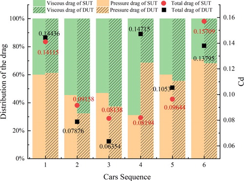
To explore the mechanism of aerodynamic drag generation, the percentage of viscous drag and pressure drag are also shown in Figure 8. As expected, the pressure drag dominated on the head and tail cars in which its contributions were about 60% and 70% of the total aerodynamic drag, respectively. This percentage for the DUT was slightly higher than that for the head car of the SUT and was lower at tail car. For the second and third cars, the air flows attaching the vehicle body again after separation, and as a result, viscous drag dominated and the proportion of the pressure drag decreased to about 48%, which was still 10% more than that of the DUT. The biggest difference found for drag distribution appeared at the fourth car, where pressure drag contributes 30% of overall drag of the fourth car for the SUT and 70% of that for the DUT. The fourth car was the most viscous-dominated car of the SUT and the most pressure-dominated car for the DUT. It has been investigated that this region has a significantly high turbulence intensity and this can be found in Guo et al. (2018). As a result, the aerodynamic drag of the fourth car was the largest among the DUT cars. After that, the pressure drag regained dominance and the fourth car of the SUT showed a higher proportion of pressure drag than that of the DUT. The tail car was found to have the highest proportion of pressure drag whether for SUT or DUT.

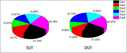
As to the overall train, $c_d$ value of DUT and SUT were 0.677 and 0.650, respectively. Thus, there was no obvious difference between the entire SUT and DUT, even though the distribution of the aerodynamic drag on each car was different. However, the use of DUT can increase the aerodynamic drag. As to the DUT, $c_d$ values of first and last three cars were 0.287 and 0.390, respectively. The pie charts, shown in Figure 9, provide the detailed proportions of the $c_d$ values of each car. The second, third, and last cars in the SUT had larger proportions of aerodynamic drag than those of the DUT, while the proportion of the fourth and fifth DUT cars were greater, where the most noticeable difference appeared at the fourth car.

Figure 9. Proportions of drag coefficient of each car.

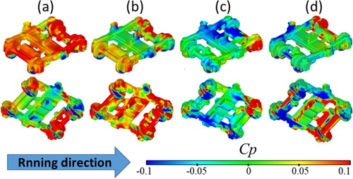
Various fatigue damage may occur during operation due to the different stress conditions. Affecting the air flow at the bottom of the train, bogies are of great importance to the aerodynamic drag on trains. Figure 10 shows the aerodynamic drag of 12 bogies in the SUT and DUT. As illustrated in Figure 10, $c_d$ values of bogies in head car was much larger than that of other bogies. Bogies of the SUT suffered from higher aerodynamic drag than those of the DUT, except for the fifth, sixth, and seventh bogies. In addition, the drag coefficients of these three bogies were larger than the adjacent two bogies (i.e. the fourth and eighth bogie) for the DUT, while it was opposite for the SUT. The difference in the drag coefficients of the bogies can be explained by the pressure distributions on their surfaces. Figure 11 shows the $c_p$ distribution on the fourth and seventh bogies, which shows the change in the $c_d$ values of the single- and double-unit train. As illustrated by Figure 11(a,b), for the fourth bogie of the SUT, there was an extensive positive pressure region on the area facing opposite to the train’s running direction, which was not found for the DUT. Thus, the SUT had a larger drag coefficient than that of the DUT. Correspondingly, more positive pressure areas and fewer negative pressure areas appeared on the same areas of the DUT, as shown in Figure 11(c,d), and as its result, the seventh bogie of SUT showed a smaller $c_d$ value.

Figure 10. Drag coefficient of the individual bogies of the SUT and DUT.

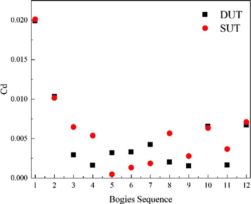
Figure 11. Distribution of the pressure on the surfaces of the bogies: (a) the fourth bogie of the SUT, (b) the fourth bogie of the DUT, (c) the seventh bogie of the SUT, and (d) the seventh bogie of the DUT.

3.3. Aerodynamic lift

The aerodynamic lift was mainly affected by the different pressure distribution on the top and bottom surfaces of a train. The dynamic axis weight of the train will increase if the negative lift is too large, intensifying the dynamic impact. However, a too large positive lift may make the contact forces generated by the train wheels and rail decrease, resulting in the phenomenon of floating, which can easily cause derailment. The lift force obtained was normalized to lift coefficient $c_l$: (3) $c_l=\frac{L}{0.5\rho {u_{in}}^{2}A}$(3) where $L$ is the aerodynamic lift for the different cars. The $c_l$ values of each car of single- and double-unit train are shown in Figure 12. The lift coefficients obtained from the SUT and DUT cars were almost the same except for those of the third car. Large pressure difference of top and bottom surfaces of head car resulted in large $c_l$ values. However, the separated flow above the tail car resulted in a large negative pressure on the top face, and this was reflected by the large positive $c_l$ value on this car. Figure 12 shows that the $c_l$ of the fourth car of single- and double-unit train were almost equal. To gain further understanding of the two lift forces, Figure 13 shows the distribution of pressure on top and bottom surfaces of the third and fourth car. Generally, a large negative lift was generated at head car while tail car experienced a positive lift. The third and fourth cars of DUT can be considered to be “fake” tail and head cars, respectively. However, as the fourth car was in a wake flow generated by the “fake” tail, the stagnation area on the nose was small compared to head car, thus a region of high surface pressure formed. Also, the flow underneath the fourth car was slower than that under the first car, resulting in a small region of negative pressure, which led to a similar value of $c_l$ of fourth car.

Figure 12. Lift coefficient of the SUT and DUT cars.

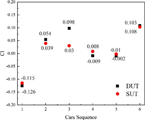
Figure 13. Distribution of the pressure on the top and bottom surfaces of the third and fourth cars.

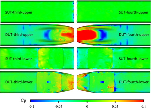
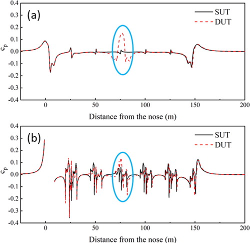
Figure 14 shows the pressure coefficient, $c_p$ above and below single- and double-unit trains at longitudinal center plane (the x–z plane at y = 0), where the height of the measurement points were 4.0 and 0.2 m, respectively. To focus on the features we concern and keep the axis range consistent, the larger measuring values at a distance around 0 were hidden in Figure 14(b). Affected by complex structures such as bogies, the bottom space of the train showed more complex flow patterns. The biggest difference appeared in the coupling region, which is marked by blue circles. For the SUT, this position is the gap downstream the third car, middle of train and far away from the nose and tail, which are known as flow-separation regions. While fort the DUT, before the coupler, between the abscissa in the 50–70 m range, the pressure decreased and a similar phenomenon appeared before the tail nose. However, this was not the real tail car, and there was still a streamlined car instead of the open air pushing the flow again and causing a sharp rise in the pressure. The upper pressure was even higher than that caused by the head nose, which was also found in Guo et al. (2019). For the bottom of the train, the maximum positive $c_p$ increased from 0.07 to 0.13 at the coupling area, and the maximum negative pressure was almost unchanged. For the top of the car, the maximum positive $c_p$ suddenly increased from 0 to 0.15, and the negative pressure also increased to a peak. The pressure change at the top was symmetric before and after the central region. However, before the central region, that is, at the lower part of the third car, the bottom pressure was always slightly positive. After the coupling region, at the lower part of the fourth car, the pressure was always slightly negative. This also created a completely different pressure distribution on the top and bottom surfaces of these two cars, which in turn formed different lift forces, as illustrated in Figure 12.

Figure 14. The pressure distribution at: (a) z = 4.0 m and (b) z = 0.2 m.

3.4. Slipstream

When the train moves at high speed, the surrounding air is dragged or squeezed and flows quickly to produce a slipstream, which is a potential safety hazard to the passengers on the platform. The value of the slipstream caused by trains is expressed in terms of the air speeds in the surrounding space and can be described as (4) $U=\frac{\sqrt{{\left(u_{in}-u\right)}^2+v^2+w^2}}{u_{in}}$(4) where $u,v,andw$ are the components of the velocity on the longitudinal, lateral, and vertical directions. There are two specific locations ($y=3.0\text{m}$ for $z$ values of $0.2$ and $1.44\text{m}$ in full-scale) mentioned by the CEN standard to assess the performance of the slipstream. The time-averaged value of U at these two positions was shown in Figure 15.

Figure 15. The value of U at measurement points required by the CEN standard: (a) y = 3.0 m, z = 0.2 m and (b) y = 3.0 m, z = 1.44 m.

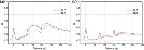
As shown in Figure 15(a), there is no difference shown on the U value of slipstream when the distance was less than 50 m, that is, this region was beyond the influence of the coupling structure. A slow increase of U value began to appear on the second car and the growth of the SUT was slightly larger than that of the DUT. When the tail of the third car passed, the DUT’s fake tail car brought a peak of U value, which is similar to the wake effect of the train. Then, the fourth car which can be regarded as a new head car pushed the air around and further increased the value of U and reached a local maximum at the end of the fourth car. Subsequently, when the last two cars of the DUT passed, the airflow velocity at this point slowly dropped until the streamline structure of the tail car passed. It is noted that the U value of the DUT was always greater than the SUT from the rear of the third car to the end of the domain, and was particularly noticeable when the latter half of the train passed. At the higher measuring point with a height of 1.44 m, except for the slipstream generated when the head car nose passed, the U value was not as large as 0.1. The main difference in U value occurred when the coupling structure passed, where the U value generated by the DUT was nearly three times that of the SUT.

3.5. Boundary layer

The boundary layer was obtained based on its definition, that is, the iso-surface where the velocity of airflow around the train body is 99% of the incoming flow velocity. The boundary layer distribution of the SUT and DUT was shown in Figure 16 in a top view (0.2 m in height) and a side view (on longitudinal symmetry plane). Only the contour of the DUT was given to mark the relative position. The black curve represented obtained boundary layer around SUT while the red represented DUT.

Figure 16. Cross-sectional profiles of the boundary layer around the SUT and DUT: (a) top view and (b) side view.

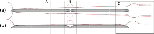
From Figure 16(a), in the width direction, the boundary layer of the SUT and DUT were kept almost the same around the first two cars. From the third car (marked by line A in the figure), the width of the boundary layer varied, the thickness of boundary layer of SUT continued to increase slowly and the width of boundary layer around DUT remained almost constant in the latter half car. As expected, the biggest difference was found around the coupling region. After passing through the nose of the third car, the width of boundary layer of DUT was sharply increased to form a spherical shape. At the fourth car right next to the coupler, the boundary layers overlapped once again, and then the thickness of the DUT began to exceed that of the SUT, and the gap became increasingly larger, except for the curved boundary layer caused by the nose of tail car. As present in Figure 16(b), the discrepancy in the height direction of the boundary layer between the SUT and DUT is not as obvious as that in width, and most of the positions are almost uniform except for a spherical boundary layer produced by the DUT in the coupling region.

3.6. Vortex structure

To understand the transient surrounding flow structure around single- and double-unit train, the vortex field must be analyzed, and the Q criterion was utilized for the purpose of identifying the vortex region, as defined in Guo et al. (2019). The iso-surfaces were established when Q is 100,000 according to the definition of Q, as shown in Figure 17. The iso-surface was rendered by the space speed coefficient, $U$, is given as: (5) $U=\frac{u_{local}}{u}$(5) where $u_{local}$ is the time-averaged velocity of train-induced slipstream and $u$ presents the speed of train.

Figure 17. Vortex structure around: (a) DUT, top view; (b) SUT, top view; (c) near wake of DUT, side view; and (d) near wake of SUT, side view.

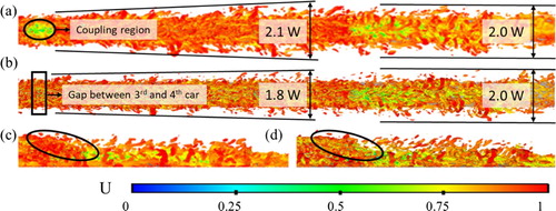
Figure 17(a,b) show the top views of the vortex structures of single- and double-unit train. When the train was moving at a constant speed, two counter-rotating vortices were generated on both sides of the head owing to the streamlined nose. No obvious differences were found between the SUT and DUT upstream the coupling structure so figures begin from the fourth car to obtain a better view. As illustrated in Figure 17(a), when the DUT was moving, a relative low speed zone was formed around the coupling region and is shown as green. The convergence of this airflow led to a pressure increase at the rear of the third car, which significantly changed its pressure resistance, making it the dominant component of the aerodynamic drag and offsetting some of the friction resistance. Therefore, the third car of the DUT showed a smaller drag, as shown in Figure 8. After the coupling structure, the vortex around the train began to shed to spanwise directions so the width of the vortex was much greater than that it was at half of the train, and this width reached 2.1 times of the train width (W) at the middle of tail car. The width of near wake vortex was unchanged at 2.0 W. As shown in Figure 17(b) for comparison, the width of the vortex was much thinner than that of the DUT, as well as the amplitude of the shedding. The vortex shedding width at the middle of tail car was 1.8 W and that of near wake was 2.0 W, which was the same of Figure 17(a). Figure 17(c,d) show the side view of the near wake vortex structure of the DUT and SUT. Higher-space speed was found attaching to the surface of tail car for the DUT, as shown in black circles. There was more complex and higher-vortex shedding behind the tail car of SUT.

4. Conclusions

DES models have been made to investigate the flow and aerodynamic forces of scaled models of the Chinese CRH2 trains for tow configurations. The single train consisted of six cars and the double-unit train consisted of two three-car trains connected by couplers. The conclusions below can be made by numerical results.

1.	The overall aerodynamic drag of double-unit train was found to be slightly larger than that of the single-unit train with the same lengths and numbers of cars. Due to the discrepancies of local pressure distribution and boundary layers, the drag coefficients of the individual cars of the DUT were different from those of the corresponding cars of the SUT. The bogies of the SUT suffered higher-aerodynamic drag than that of DUT, except for the fifth, sixth, and seventh bogies.
2.	Most of the cars of single- and double-unit trains suffered from approximately the same aerodynamic lift forces, while the lift of the front car closely upstream the coupler was more than three times that of single-unit train. This was result from large pressure under the bottom of the front car closely upstream the coupler.
3.	The coupling structure can bring an obvious increase in the time-averaged velocity magnitudes of the slipstream of the DUT. The value of U increased in the following regions (around the last three cars and the wake region).
4.	Up to the coupler, boundary layer’s thickness on two sides of double-unit train along its length was similar to that of the SUT. After the coupler, the DUT exhibited a larger boundary layer thickness. The boundary layer thicknesses above the two trains were almost the same except for a small region above the coupler, in which a large boundary layer thickness was found above the DUT.
5.	The development of the vortex structure around the train was similar with the law of the development of a boundary layer. The differences in the widths in the vortex region between the SUT and DUT were relatively obvious compared to the height, and there was greater vortex-shedding around the DUT.
6.	There are some points not well thought out, such as the sensitivity of the train configuration including head car shape, gaps between cars, or train length, and that they can indeed give a potential influence on surrounding flow around trains, especially double-unit trains. Although the length of trains we used in this study meets the criteria for simulation. However, due to the presence of the boundary layers, the longer the train, the more uncontrollable the vehicle drag is. The influence of the train length for the double unit trains will be studied next.

Disclosure statement

No potential conflict of interest was reported by the author(s).

Additional information

Funding

This work was supported by National Natural Science Foundation of China: [grant number 11902367]; Ministry of Science and Technology of the People's Republic of China: [grant number 2016YFB1200504].

References

- Akbarian, E., Najafi, B., Jafari, M., Faizollahzadeh Ardabili, S., Shamshirband, S., & Chau, K.-W. (2018). Experimental and computational fluid dynamics-based numerical simulation of using natural gas in a dual-fueled diesel engine. Engineering Applications of Computational Fluid Mechanics, 12(1), 517–534. https://doi.org/10.1080/19942060.2018.1472670
- Baker, C., Quinn, A., Sima, M., Hoefener, L., & Licciardello, R. (2013a). Full-scale measurement and analysis of train slipstreams and wakes. Part 1: Ensemble averages. Proceedings of the Institution of Mechanical Engineers, Part F: Journal of Rail and Rapid Transit, 228(5), 451–467. https://doi.org/10.1177/0954409713485944
- Baker, C., Quinn, A., Sima, M., Hoefener, L., & Licciardello, R. (2013b). Full-scale measurement and analysis of train slipstreams and wakes. Part 2 Gust analysis. Proceedings of the Institution of Mechanical Engineers, Part F: Journal of Rail and Rapid Transit, 228(5), 468–480. https://doi.org/10.1177/0954409713488098
- CEN. (2011). Railway applications – Aerodynamics – Part 4: Requirements and test procedures for aerodynamics on open track.
- Chen, Z., Liu, T., Zhou, X., & Su, X. (2016). Aerodynamic analysis of trains with different streamlined lengths of heads. In 2016 IEEE international conference on Intelligent Rail Transportation (ICIRT). https://doi.org/10.1109/ICIRT.2016.7588758
- Deng, E., Yang, W., Deng, L., Zhu, Z., He, X., & Wang, A. (2020). Time-resolved aerodynamic loads on high-speed trains during running on a tunnel–bridge–tunnel infrastructure under crosswind. Engineering Applications of Computational Fluid Mechanics, 14(1), 202–221. https://doi.org/10.1080/19942060.2019.1705396
- Deng, E., Yang, W., Lei, M., Zhu, Z., & Zhang, P. (2019). Aerodynamic loads and traffic safety of high-speed trains when passing through two windproof facilities under crosswind: A comparative study. Engineering Structures, 188, 320–339. https://doi.org/10.1016/j.engstruct.2019.01.080
- Flynn, D., Hemida, H., Soper, D., & Baker, C. (2014). Detached-eddy simulation of the slipstream of an operational freight train. Journal of Wind Engineering and Industrial Aerodynamics, 132, 1–12. https://doi.org/10.1016/j.jweia.2014.06.016
- Ghalandari, M., Shamshirband, S., Mosavi, A., & Chau, K.-W. (2019). Flutter speed estimation using presented differential quadrature method formulation. Engineering Applications of Computational Fluid Mechanics, 13(1), 804–810. https://doi.org/10.1080/19942060.2019.1627676
- Guo, Z., Liu, T., Chen, Z., Liu, Z., Monzer, A., & Sheridan, J. (2020a). Study of the flow around railway embankment of different heights with and without trains. Journal of Wind Engineering and Industrial Aerodynamics, 202, 104203. https://doi.org/10.1016/j.jweia.2020.104203.
- Guo, Z., Liu, T., Chen, Z., Xia, Y., Li, W., & Li, L. (2020b). Aerodynamic influences of bogie’s geometric complexity on high-speed trains under crosswind. Journal of Wind Engineering and Industrial Aerodynamics, 196, 104053. https://doi.org/10.1016/j.jweia.2019.104053.
- Guo, Z.-J., Liu, T.-H., Chen, Z.-W., Xie, T.-Z., & Jiang, Z.-H. (2018). Comparative numerical analysis of the slipstream caused by single and double unit trains. Journal of Wind Engineering and Industrial Aerodynamics, 172, 395–408. https://doi.org/10.1016/j.jweia.2017.11.022
- Guo, Z., Liu, T., Yu, M., Chen, Z., Li, W., Huo, X., & Liu, H. (2019). Numerical study for the aerodynamic performance of double unit train under crosswind. Journal of Wind Engineering and Industrial Aerodynamics, 191, 203–214. https://doi.org/10.1016/j.jweia.2019.06.014
- Hemida, H., Baker, C., & Gao, G. (2012). The calculation of train slipstreams using large-eddy simulation. Proceedings of the Institution of Mechanical Engineers, Part F: Journal of Rail and Rapid Transit, 228(1), 25–36. https://doi.org/10.1177/0954409712460982
- Hemida, H., & Krajnović, S. (2010). LES study of the influence of the nose shape and yaw angles on flow structures around trains. Journal of Wind Engineering and Industrial Aerodynamics, 98(1), 34–46. https://doi.org/10.1016/j.jweia.2009.08.012
- Krajnović, S., Ringqvist, P., Nakade, K., & Basara, B. (2012). Large eddy simulation of the flow around a simplified train moving through a crosswind flow. Journal of Wind Engineering and Industrial Aerodynamics, 110, 86–99. https://doi.org/10.1016/j.jweia.2012.07.001
- Li, C., Burton, D., Kost, M., Sheridan, J., & Thompson, M. (2017). Flow topology of a container train wagon subjected to varying local loading configurations. Journal of Wind Engineering and Industrial Aerodynamics, 169, 12–29. https://doi.org/10.1016/j.jweia.2017.06.011
- Li, T., Hemida, H., Zhang, J., Rashidi, M., & Flynn, D. (2018). Comparisons of shear stress transport and detached Eddy simulations of the flow around trains. Journal of Fluids Engineering, 140(11), Article 111108. https://doi.org/10.1115/1.4040672
- Li, T., Qin, D., & Zhang, J. (2019). Effect of RANS turbulence model on aerodynamic behavior of trains in crosswind. Chinese Journal of Mechanical Engineering, 32(1), 85. https://doi.org/10.1186/s10033-019-0402-2
- Li, T., Qin, D., Zhang, W., & Zhang, J. (2020). Study on the aerodynamic noise characteristics of high-speed pantographs with different strip spacings. Journal of Wind Engineering and Industrial Aerodynamics, 202, 104191. https://doi.org/10.1016/j.jweia.2020.104191
- Li, R., Xu, P., Peng, Y., & Ji, P. (2016). Multi-objective optimization of a high-speed train head based on the FFD method. Journal of Wind Engineering and Industrial Aerodynamics, 152, 41–49. https://doi.org/10.1016/j.jweia.2016.03.003
- Liu, T.-H., Jiang, Z.-H., Li, W.-H., Guo, Z.-J., Chen, X.-D., Chen, Z.-W., & Krajnovic, S. (2019). Differences in aerodynamic effects when trains with different marshalling forms and lengths enter a tunnel. Tunnelling and Underground Space Technology. https://doi.org/10.1016/j.tust.2018.10.016
- Mao, J., Xi, Y., & Yang, G. (2012). Numerical analysis on the influence of train formation on the aerodynamic characteristics of high-speed trains under crosswind. Zhongguo Tiedao Kexue/China Railway Science, 33, 78–85. https://doi.org/10.3969/j.issn.1001-4632.2012.01.12
- Mou, B., He, B.-J., Zhao, D.-X., & Chau, K.-W. (2017). Numerical simulation of the effects of building dimensional variation on wind pressure distribution. Engineering Applications of Computational Fluid Mechanics, 11(1), 293–309. https://doi.org/10.1080/19942060.2017.1281845
- Muld, T., Efraimsson, G., & Henningson, D. (2013). Wake characteristics of high-speed trains with different lengths. Proceedings of the Institution of Mechanical Engineers, Part F: Journal of Rail and Rapid Transit, 228(4), 333–342. https://doi.org/10.1177/0954409712473922
- Niu, J., Wang, Y., & Liu, F. (2020). Numerical study on the effect of damaged windows on aerodynamic characteristics of passenger trains under strong crosswind. Proceedings of the Institution of Mechanical Engineers, Part C: Journal of Mechanical Engineering Science. Article 095440622091139. https://doi.org/10.1177/0954406220911396
- Niu, J., Wang, Y., Liu, F., & Li, R. (2020a). Numerical study on the effect of a downstream braking plate on the detailed flow field and unsteady aerodynamic characteristics of an upstream braking plate with or without a crosswind. Vehicle System Dynamics, 1–18. https://doi.org/10.1080/00423114.2019.1708959.
- Niu, J., Wang, Y., Wu, D., & Liu, F. (2020b). Comparison of different configurations of aerodynamic braking plate on the flow around a high-speed train. Engineering Applications of Computational Fluid Mechanics, 14(1), 655–668. https://doi.org/10.1080/19942060.2020.175641.
- Niu, J., Zhou, D., Liu, T., & Liang, X.-F. (2017). Numerical simulation of aerodynamic performance of a couple multiple units high-speed train. Vehicle System Dynamics, 55(1), 1–23. https://doi.org/10.1080/00423114.2016.1277769
- Sicot, C., Delinacourt, F., Jacques, B., Aguinaga, S., & Bouchet, J.-P. (2018). Representativeness of geometrical details during wind tunnel tests. Application to train aerodynamics in crosswind conditions. Journal of Wind Engineering and Industrial Aerodynamics, 177, 186–196. https://doi.org/10.1016/j.jweia.2018.01.040
- Zhang, J., Li, J.-J., Tian, H.-Q., Gao, G.-J., & Sheridan, J. (2016). Impact of ground and wheel boundary conditions on numerical simulation of the high-speed train aerodynamic performance. Journal of Fluids and Structures, 61, 249–261. https://doi.org/10.1016/j.jfluidstructs.2015.10.006
- Zhang, L., Yang, M.-Z., & Liang, X.-F. (2018). Experimental study on the effect of wind angles on pressure distribution of train streamlined zone and train aerodynamic forces. Journal of Wind Engineering and Industrial Aerodynamics, 174, 330–343. https://doi.org/10.1016/j.jweia.2018.01.024