A numerical study for the assessment of air pollutant dispersion with chemical reactions from a thermal power plant

Abstract

In this work, a computational simulation of the pollutants spread generated during fuel combustion at Ekibastuz SDPP-1 and their chemical reaction in the atmosphere have been presented. Using the example of a real thermal power plant (Ekibastuz SDPP -1), the dispersion NO, NO₂, CO and products NO₂, HNO₃, CO₂ during a chemical reaction with oxygen was modeled. The numerical method was verified by solving three test problems and the received computational solutions were compared with data from the measurement and the computational data of other authors. The purpose of the work was to investigate the pollution level at various ranges from the source. As a result, the mass fraction of the concentration and product during a chemical reaction were determined. According to the obtained data, with increasing distance from the source, the concentration of pollution spreads more widely under the influence of diffusion. The farther the distance from the chimney, the lower the concentration of the substance and products. Thus, the obtained computational values may allow in the future predicting the optimal distance from residential areas for the construction of thermal power plants, at which the concentration of emissions will remain at a safe level.

KEYWORDS:

• Chemical reaction
• air pollutant dispersion
• thermal power plant
• jet in crossflow
• Reynolds averaged Navier-Stokes (RANS)

1. Introduction

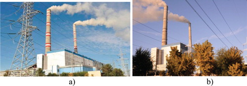
Atmospheric air is a vital component of the natural environment. The continuous negative impact on the atmosphere and the unsatisfactory resolution of issues related to its improvement negatively affect the health of the population. Air pollution is created from the activities of industrial enterprises, power plants, cars, which emit hundreds of tons of harmful substances into the atmosphere. Photochemical processes constantly occur in the air basin, leading to the emergence of new compounds, sometimes more harmful than the initial ones. Thermal power plants (TPPs) are one of the main sources of environmental pollution (Figure 1). Thermal power plants produce electricity (up to 75% of the total world electricity generation) and thermal energy. When burning, the bulk of the fuel is converted into waste that enters the environment in the gaseous and solid combustion products form. When burning fuel, a large amount of oxygen is consumed, and a significant amount of combustion products are released.

Figure 1. Ekibastuz SDPP-1, Kazakhstan.

Air pollutants can be divided into couple classes. The first class includes primary air pollutants (Akbarian et al., 2018; Ghalandari et al., 2019; Mayer, 1999; Mou et al., 2017), which are ejected into the environment directly from emission source (usually from fuel combustion) and mainly contain of particulate matter components, carbon monoxide (CO), volatile organic compounds (VOCs) and nitrogen oxides (NOx) – mainly NO (Dunmore et al., 2015). The next class is auxiliary air pollutants that form in the environment, while primary air pollutants undergo physical and chemical reactions (Jacobson, 2005). Chemical reactions lead to the dilution of reagents and the formation of secondary pollutants, which are functions of the pollutants concentration, temperature and chemical kinetics (Fiorina et al., 2015; Wu & Liu, 2018). One of the significant auxiliary air pollutant is Ozone (O₃), which is formed as a result of chemical reactions, containing basically the oxidation of NOx and VOCs in the sunlight presence. Reactive intermediates (hydroxyl (OH) and hydroperoxyl (HO₂) radicals) regulate the chemical decomposition cycle, converting NO to NO₂ and, consequently, the formation of O₃ (Bloss, 2009). In the papers (Li, Li et al., 2018, 2019; Muñoz et al., 2018) the formation mechanisms NO₂ in the chemical composition have been numerically investigated, which consisted of 45 species and 142 reactions. The approved model has been applied to form NO₂ from NO. So nitrogen oxides are greenhouse gases, but these pollutants also react with organic compounds to form smog (ground-level ozone). The sulfur dioxide and nitrogen oxides contribute to the appearance of acid rain. The share of combined heat and power (CHP) plant in anthropogenic emissions of these oxides is 15–45% and 45–65%, respectively (U.S. Environmental Protection Agency). When these pollutants mix with oxygen, water and other chemicals in the air, it forms acids. The oxygen is characterized by high chemical activity, and the air contains 21% oxygen. It should be borne in mind that many substances react with oxygen at room temperature. As a result of chemical interaction of substances with oxygen, new harmful ingredients that are more dangerous for humans can be synthesized. Therefore, the problems of atmospheric air pollution and the implementation of measures to clean it remain relevant today.

However, it should be taken into account that if TPPs are located inside or near a city, then one of the main factors affecting the distribution of concentration will be the surrounding buildings and the location of the building (Li et al., 2008b). Since constructions are man-made barriers to urban atmospheric flow and lead to limited ventilation, particularly for deep street canyons (Salim et al., 2011). The deterioration of urban air quality is due to the combined effects of traffic emissions, dynamics of emissions and chemical composition in the environment (Li et al., 2008b). The study on air pollution in street canyons due to their great practical importance has been examined experimentally, numerically and theoretically in many papers (Ahmad et al., 2005; Bright et al., 2013; Kwak et al., 2013; Li et al., 2012; Vardoulakis et al., 2003; Yazid et al., 2014; Zhong et al., 2016). In paper (Wegner & Huai, 2016) a chemical reactive pollutant was numerically investigated that relates to the dynamics of street canyons. Moreover, the LES model was used to study the dispersion and transfer of reactive O₃, NO₂, NO species in the deep canyon of a city street by connecting with simple NOx-O₃ chemical compounds (Li et al., 2008a; Zhong et al., 2015). Furthermore in works (Kikumoto & Ooka, 2012; Kim et al., 2012; Zhong et al., 2015), using the LES method, simulated the effects of bimolecular chemical reactions on concentration and transport pollutant gases to disperse air pollutants in the atmospheric boundary layer.

There are a several methods for solving like that kind of problems, among which one can distinguish a three dimensional experiment, computational simulation and theoretical investigations. The empirical approach includes conducting a real measurement on actual states, using the required devices and fixtures, making measurements of the required values. Nevertheless, this approach is very complex and very expensive way. Moreover, in densely populated places such experiments are extremely inconvenient, because of the air quality in urban conditions basically depends on the wind flow. Theoretical approaches could be determined by methods such as the semi-empirical model and the Gaussian model, but these are unsatisfactory for accurate pollutant prediction. Thus, for a more profitable and efficient investigation of environmental problems, computational simulation is preferred because of its flexibility in calculations, and so it is not so expensive viable method, which makes it much more convenient.

So from these works, the reactivity of air pollutants was revealed that have a significant effect on the concentration value, thus, the concentration of products in the canyon space was higher than the concentration value of the reactants. This effect is due to a stably circulating stream in the canyon, which promotes the reactive gases mixing, and the reactions take place during the time in which the reactors are held. So (Liu et al., 2017) simulated the formation of synthesis gases, such as CO, CO₂, H₂, CH₄ and C₂H₄. The results of transient processes simulation show that an excess of steam accelerates the gasification of coal and accelerates the reaction; therefore, an optimal steam flow should be chosen as a compromise between the reaction time and the quality of synthesis gas. While in the other works (Mărunţălu et al., 2015; Shi et al., 2006, 2007), gas-phase chemical reactions were simulated. Also in paper (Bulat et al., 2014) used the same strategy to study the production of CO and NOx. So the mechanisms and kinetics of gas-phase reactions O₃ have been the subject of numerical investigations over the past years (Atkinson & Carter, 1984; Atkinson, 1989, 1990; Bahta et al., 1984; Bennett et al., 1987; Gillies et al., 1988; Grosjean, 1990; Hatakeyama &  Akimoto, 1990; Horie & Moortgat, 1991; Izumi et al., 1988; Martinez & Herron, 1988; Niki et al., 1983; Nolting et al., 1988; Paulson et al., 1992; Shorees et al., 1991; Yokouchi & Ambe, 1985; Zozom et al., 1987). Currently, one of the main uncertainties relates to reactions in the atmospheric conditions of biradicals, the degree and nature of decomposition products. There is evidence of product and kinetic studies that reactive radical species are formed during these reactions (Atkinson et al., 1990a; Herron & Huie, 1978; Martinez et al., 1981; Martinez & Herron, 1988; Niki et al., 1987; Paulson et al., 1992), and OH radicals play an important role in this chemical reaction.

However, it should be noted that in order for these elements to enter a chemical reaction, certain atmospheric conditions will be necessary. And another thing to remember is certain conditions during the combustion of fuel. So at the moment, various technologies of oxygen combustion are used in order to reduce carbon dioxide (CO₂) emissions from chimneys. This method is also a promising method for eliminating NOx emissions (Andersson & Johnsson, 2006, 2007; Habib et al., 2017). The combustion process using CFD (Al-Abbas et al., 2011) is a very important process, since the investigation of the combustion reaction mechanisms and the emission model are very important for accurate prediction of the combustion characteristics (Ditaranto & Oppelt, 2011; Khalil & Gupta, 2017a; Khalil & Gupta, 2017b; Kim et al., 2007; Li, Shi et al., 2018; Smith et al., 1999). However, taking into account the entire combustion process in modeling is currently very resource-intensive and a set of simplified chemical mechanisms is usually used to reduce computational efforts (Andersen et al., 2009; Frassoldati et al., 2009). However, it should be noted that carbonyl sulphide (COS), carbon disulphide (CS₂) and carbon monoxide (CO) chemical compounds are formed in reactions involving carbon dioxide (CO₂) and hydrocarbons present in the acid gas stream (Goar, 1989; Goar & Hyne, 1996; Maddox, 1998).

A detailed review of works presented the investigating of the substances flow leaving the pipe in a transverse flow was found in work (Denev et al., 2006). In papers (Andreopoulos & Rodi, 1984; Kelso et al., 1996; Muppidi & Mahesh, 1999; Muppidi & Mahesh, 2008) numerically investigated the velocity field, and in works (Crabb et al., 1981; Majander & Siikonen, 2006; Sherif & Pletcher, 1989) modeled a passive scalar field of concentration. In the article (Yuan et al., 1999; Ziefle & Kleiser, 2009), numerical simulation is performed using the large eddy simulation (LES) method, which gives best values than other methods. The simulation was carried out at two ratios of jet velocity to transverse flow, 2.0 and 3.3, and two different Reynolds numbers (1050, 2100) based on the transverse flow velocity and jet diameter. In paper (Keffer & Baines, 1963), jet trajectories and velocity along it were measured. A complete study was conducted in (Crabb et al., 1981), which measured the mean and fluctuating velocity values using a laser Doppler anemometer near the jet exit. In paper (Wegner & Huai, 2004) turbulent mixing was studied using the LES method. They changed the angle between the stream and the cross flow. The mixing intensified as the angle increased, that is, when the jet was directed against the cross flow. The received numerical data were compared with measurement data (Andreopoulos & Rodi, 1984).

To simulate such real size problems, it is necessary to solve test problems. By these test problems were verified the accuracy of the numerical algorithm. For this objective, in this work, 2D and 3D test problems of the pollutants movement which is exiting from the pipe, perpendicular to the main flow in the channel were investigated. The calculations were performed using the ANSYS Fluent. The obtained data were compared with values from the experiment. Satisfactory agreement with data from measurement was obtained. The values showed a closer agreement with the measurement values than the values of simulations by other authors.

Then, modeling of atmospheric pollution at Ekibastuz SDPP-1 was performed (Figure 1). This power plant is the biggest TPP in the Republic of Kazakhstan Ekibastuz city, Pavlodar region, located on the northern side of the Zhyngyldy Lake, 16 km north of Ekibastuz city. The operating capacity of Ekibastuz SDPP-1 is about 3,500 MW. Construction dimensions: height – 64.0 m, length – 500.0 m and width – 132.0 m. Chimney height: 300.0 m (built in 1980) and 330.0 m (built in 1982). The various heights of chimneys allowed studying the influence of the source height on the pollution dispersion.

2. Mathematical model

CFD modeling of these processes is based on the Navier – Stokes equations, consisting of the continuity and momentum equations (Chung, 2002; Ferziger & Peric, 2013; Issakhov, 2014, 2016; Issakhov et al., 2018; Issakhov & Imanberdiyeva, 2019).

• The continuity equation: (1) $\frac{\mathrm{\partial }{u}_j}{\mathrm{\partial }{x}_j}=0$(1) • The momentum equation: (2) $\begin{array}{rl}& \frac{\mathrm{\partial }\rho u_i}{\mathrm{\partial }t}+\frac{\mathrm{\partial }}{\mathrm{\partial }{x}_j}\left(\rho u_i{u}_j\right)\\ & =-\frac{\mathrm{\partial }{p}^{\mathrm{\prime }}}{\mathrm{\partial }{x}_i}+\frac{\mathrm{\partial }}{\mathrm{\partial }{x}_j}\left({\mu }_{eff}\left(\frac{\mathrm{\partial }{u}_i}{\mathrm{\partial }{x}_j}+\frac{\mathrm{\partial }{u}_j}{\mathrm{\partial }{x}_i}\right)\right)-\rho \overrightarrow{g}\stackrel{⌢}{n}\end{array}$(2) where $p^{\mathrm{\prime }}$ is the modified pressure and ${\mu }_{eff}$ the effective viscosity. Here $p^{\mathrm{\prime }}=p+\left(2/3\right)\rho k+\left(2/3\right){\mu }_{eff}\left(\mathrm{\partial }{u}_k/\mathrm{\partial }{x}_k\right)$ and ${\mu }_{eff}=\mu +{\mu }_t$, where ${\mu }_t=C_{\mu }\rho \left(k^2/\epsilon \right)$ the turbulence viscosity, $u_i$ velocity components, $\rho$ density, $\overrightarrow{g}$ gravitational force, $\stackrel{⌢}{n}$ normal vector. To carry out this simulation, the temperature dependence was not used, and the temperature was taken as T = 300 K. In order to close the system of the equation a different turbulent models have been applied.

• Chemical reaction:

To account for the chemical reaction, substance B is used, coming out of the pipe, which reacts with substance A of the main flow, as a result substance C is formed. This chemical reaction can be written in this form: $A+B\stackrel{k}{\to }C$where k is the kinetic reaction rate, which is determined by the Arrhenius equation, which is given by $k=A{T}^{b}ex{p}^{\frac{-E_a}{RT}}$where A is the pre-exponential reaction coefficient (${10}^{15}$), T is the temperature in Kelvin, b is the temperature coefficient, R is the universal gas constant, $E_a$ is the activation energy for the reaction (${10}^8$).

• The species equations:

To calculate the species transfer with the chemical reaction, equations for the components $Y_1$ and $Y_2$ taking into account the chemical kinetics of the reaction were used. (3) $\frac{\mathrm{\partial }\rho Y_i}{\mathrm{\partial }t}+\frac{\mathrm{\partial }}{\mathrm{\partial }{x}_j}\left(\rho u_i{Y}_i\right)=\frac{\mathrm{\partial }}{\mathrm{\partial }{x}_j}\left(D_{eff}\left(\frac{\mathrm{\partial }{Y}_i}{\mathrm{\partial }{x}_j}\right)\right)+{\omega }_i$(3) where ${\omega }_i=-k_i{Y}_1{Y}_2$.

The resulting product concentration $Y_3$ is calculated according to the Dalton law: (4) $Y_3=1-Y_1-Y_2$(4) The system of equations is used the Cartesian coordinate system $x_i$ (i = 1, 2, 3), in physical space; $Y_i$ the components of species, three components of velocity $u_i,$ p – pressure; μ is the dynamic viscosity, $\vartheta =\mu /\rho$ – is the kinematic viscosity, ρ is the density, μ is the diffusion coefficient, t is the dimensionless time, $D_{eff}=\left(\rho D_{i,m}+\left({\mu }_t/S{c}_t\right)\right)$, where $S{c}_t=\left({\mu }_t/\rho D_t\right)$ – turbulent Schmidt number ($D_t$ – the turbulent diffusivity). The $S{c}_t$ by default is 0.7.

3. Turbulent models

In order to close the system Equations (1)–(4) several turbulent models have been used. It was used different turbulent model:

1. For $k-\epsilon$ turbulent model (k – kinetic turbulent energy and ϵ – turbulent dissipation rate) (Issakhov et al., 2019a, 2019b; Issakhov et al., 2020; Issakhov & Mashenkova, 2019; Issakhov & Omarova, 2020; Launder & Spalding, 1974).

2. For SST $k-\omega$ turbulent model (k- kinetic turbulent energy and ω – the specific dissipation rate) (Issakhov & Mashenkova, 2019; Issakhov & Omarova, 2020; Issakhov & Zhandaulet, 2020a, 2020b, 2020c; Menter, 1993, 1994).

4. Numerical method

The SIMPLE numerical algorithm (semi-explicit method for pressure related equations) by Patankar and Spalding (Patankar, 1980) was used to numerical solve the equations system (1)–(4). The use of this numerical algorithm is described in detail (Issakhov & Baitureyeva, 2019; Issakhov & Mashenkova, 2019; Issakhov & Zhandaulet, 2019; Issakhov et al., 2019a; Muhammad et al., 2020).

5. Test problem for the velocity field

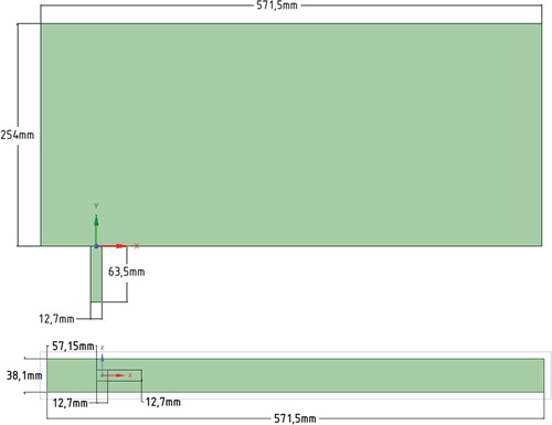
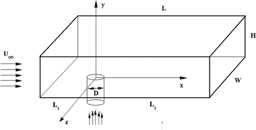
For a more accurate implementation of the selected problem study, the values were first obtained on the basis of the available data from the papers (Ajersch et al., 1995; Keimasi & Taeibi-Rahni, 2001). The test problem area was the 3D channel with a pipe inside it. The area’s parameters as follows: the main channel height 20D, the main channel length 45D, the main channel width 3D, the height of the vertical channel 5D, and the center of the vertical channel is at a distance of 5D from the inlet. The vertical channel was square, with the diameter D = 12.7 mm (Figure 2).

Figure 2. Parameters of the calculated area.

Furthermore, the structured grid was constructed in order to obtain an accurate value: the transverse channel consists of 315 × 140 × 21 nodes, the vertical channel consists of 7 × 35 × 7 nodes, the total number of elements is 926031 (Figure 3).

Figure 3. The computational domain grid.

5.1. Boundary conditions

In paper (Keimasi and Taeibi-Rahni) considered different ratios of jet velocity to transverse flow R (0.5, 1.0, and 1.5). In this study, the ratio R = 0.5 was used; at this ratio, the jet velocity was 5.5 m/s, the cross flow velocity was 11.0 m/s. The air was selected as the medium. The diameter of vertical channel (D) was 12.7 mm. The Reynolds number was determined like that: $Re=\left(\right(\rho V_{jet}D\left)/\mu \right)=4700$. To represent the inlet velocity profile of the transverse flow the 1/7 power law of the wind in the boundary layer was used. $\frac{u}{u_r}={\left(\frac{z}{z_r}\right)}^{\alpha }$At a height more than 2D, the U-velocity was set to a stationary and determined like 11.0 m/s. The V-velocity for the vertical channel was set to a stationary and determined like 5.5 m/s (Figure 4). Here u is the wind speed at the height z, and $u_r$ is the known wind speed at the reference height $z_r$. $\alpha$ _– empirically derived coefficient, which changes depending on the atmosphere stability. Here $\alpha =1/7$ for conditions of neutral stability (Figures 4 and 5).

Figure 4. Boundary conditions of the reactor (OXY plane).

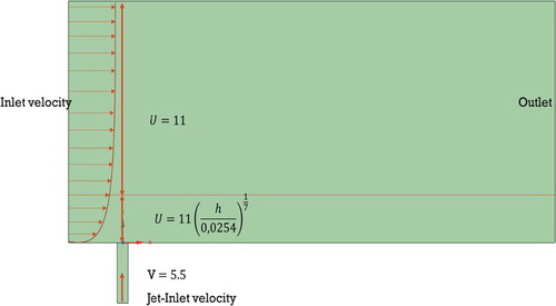
Figure 5. Boundary conditions of the reactor (OYZ plane).

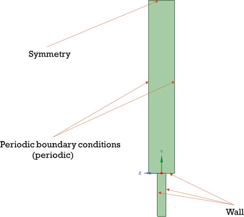
These velocity values were set to repeat the measurement done by (Ajersch et al., 1995). At the entrance boundary of the horizontal flow, conditions were set on the components of the (k-ω)/(k-ϵ) models.

During calculations using the k-ϵ turbulent model, the following initial condition were specified. For turbulent kinetic energy profile was occurred that relies on the initial velocity in order to receive closest agreement with the experiment by (Ajersch et al., 1995). $k=\left\{\begin{array}{ll}\left(0.3+0.3{\left(\frac{0.008-y}{0.0254}\right)}^{\frac{1}{7}}\right)V_{hor}& y<0.008\\ 0.3\cdot V_{hor}& y=0.008\\ 0.3-0.3\cdot {\left(\frac{y-0.008}{0.0254}\right)}^{\frac{1}{7}}{V}_{hor}& \begin{array}{c}0.008<y\\ <0.0254\end{array}\\ 0.0012\cdot V_{hor}& y>0.0254\end{array}\right.$The boundary conditions for dissipate turbulent energy was used like in paper (Versteeg & Malalasekera, 1996): ${\epsilon }_{in}=C_{\mu }^{\frac{3}{4}}\left(k^{\frac{3}{2}}/L_m\right)$where C_μ = 0.09 is an empirical constant.

For the boundary conditions operating as a ‘wall’, the standard conditions were selected, which are offered by the ANSYS Fluent. The periodic boundary conditions for the horizontal channel on the Z axis were established.

The following initial conditions were used for simulation the k-ω turbulent model. For the dissipation rate of turbulent energy, a formula was set that was proposed by (Menter, 1994): $\omega =(1\to 10)\left(V_{hor}/L\right),$where L is the reactor length. The horizontal acceleration at the outlet boundary was determined as 0.

5.2. Comparison of numerical results

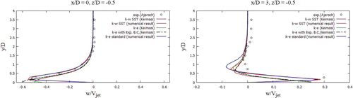
The received computational values were compared with the computational values (Keimasi & Taeibi-Rahni, 2001) and values from the measurement studies (Ajersch et al., 1995). In Figure 6, the U-velocity profiles for various turbulent models were matched, the received computational values agree well with the measured values for the transverse section x/D = 0, z/D = 0 (Ajersch et al., 1995), but for the transverse section x/D = 3, z/D = 0 as it can be seen there are several differences in a data. From Figure 7, it could be noted that the V-velocity profiles for various turbulent models characterize the flow behavior well, but, however, deviations from empirical values appear in all turbulence models (Ajersch et al., 1995), except for the SST k-w turbulent model. Among the received computational data using various turbulent models (Figure 7), it is worth highlighting the SST k- w turbulent model, the computational data of this model are closest to the measured values for all cross sections (Ajersch et al., 1995). From Figure 8 it can be noted that the received computational data by the SST k-w model for the V-velocity agree well with the measured values (Ajersch et al., 1995).

Figure 6. Comparison of the profile of U-velocity for various transverse sections.

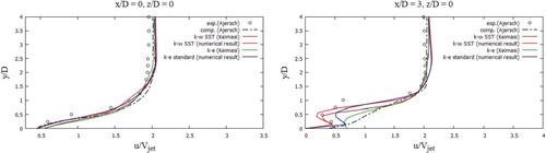
Figure 7. Comparison of the profile of V-velocity for various transverse sections.

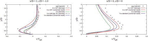
Figure 8. Comparison of the profile of W-velocity for various transverse sections.

During verification of turbulent models (Figures 6–8), the SST k-w model turned out to be the closest and optimal model. In the future, the turbulent SST k-w model was applied for the problem in real sizes, since the LES turbulent model captures low-frequency parameter changes, unlike RANS, when constant average values are obtained, and large computational power is expended.

6. Test problem for the velocity field and concentration components

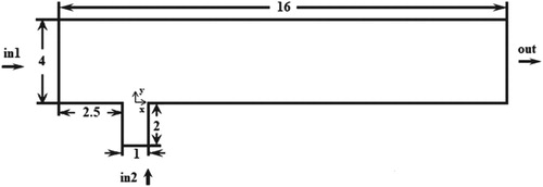
This section discusses the following test problem. A detailed description of this test problem and experiment is given in (Crabb et al., 1981; Majander & Siikonen, 2006). The test problem area was 3D channel with a pipe inside it. The pipe diameter (jet width) was D = 12.7 mm, which was used as a unit of length. The height of the transverse channel H = 7D, the height of the pipe 2D, the length of the transverse channel L = 13D, the width of the channel W = 8D, and the center of the vertical channel is at a distance $L_1$ = 3D from the entrance (Figure 9).

Figure 9. Map of the calculated area.

Air was chosen as the computational material for the transverse flow, and water vapor for the jet. For the numerical simulation of this problem, the following parameters were taken: dynamic air viscosity was $\mu =1.7894\times {10}^{-5}$ kg·${\text{m}}^2$/sec, density ρ = 1.225 kg/${\text{m}}^3$; the dynamic viscosity of water vapor is $\mu =1.34\times {10}^{-5}$ kg·${\text{m}}^2$/sec, density ρ = 0.5542 kg/${\text{m}}^3$. The initial temperature was selected as 300 K. The Reynolds number was defined as $R{e}_{jet}=\rho V_{jet}D/\mu =46700$ (Crabb et al., 1981; Majander & Siikonen, 2006).

6.1. Construction of the computational grid

An unstructured grid was built for the simulation and was thickened near the wall, around the exit of the pipe and along the ejection path (the size of the computational grid is up to 17 cm). The total number of three-dimensional cells is more than 1054656 elements (Figures 10 and 11).

Figure 10 Computational grid of the computational domain.

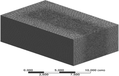
Figure 11. (a) horizontal section and (b) vertical section in the central plane, z/D = 0.

6.2. Boundary conditions

To describe the initial velocity profile of the jet, the profile of the substance in the form of an exponent was used. $v_y=v\ast (1-e^{-1510\zeta }),\zeta =min(x;L_x-x)$The initial velocity profile of the transverse flow is given as a constant. The ratio of jet velocity to cross flow velocity was determined like $R=V_{jet}/V{}_{crossflow}$. For this test problem, the ratio is taken as R = 2.3, so the jet velocity was 53.7 m/s, the cross-flow velocity was 23.35 m/s. The remaining boundary conditions are displayed in Figure 12. So the boundary conditions for the jet are taken as the concentration of water vapor is 1, and the concentration of the transverse air flow is taken as 0. And for the cross-flow, the boundary conditions are taken as the concentration of water vapor is taken as 1.

Figure 12. Boundary conditions of the reactor (OYZ plane).

6.3. Comparison of numerical results

Figure 13 compares the mean horizontal velocity profiles with experimental data (Crabb et al. (1981)) and numerical data that were solved using the LES turbulent model (Majander & Siikonen,  2006) with the obtained numerical data in this work for different sections x/D = {−1, 0, 0.5, 0.75, 1, 1.5, 4, 6, 8} and z/D = 0. In Figure 14, the mean concentration profiles were compared with measured values (Crabb et al., 1981) and numerical values that were solved using the LES turbulent model (Majander & Siikonen, 2006) with obtained numerical data in this work for different sections x/D = {1, 2, 4, 6, 8, 10} and z/D = 0. From all the obtained computational values, it can be noted that the received values using the SST k-w turbulent model for the U-velocity agree adequately with the empirical data (Crabb et al., 1981).

Figure 13. Mean flow rates in the central plane, z/D = 0: (Crabb et al., 1981) (o), Majander & Siikonen (2006) (-) LES (-).

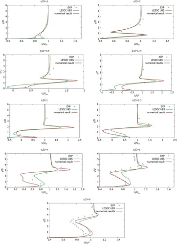
Figure 14. The mean proportion of the mixture in the central plane, z/D = 0: (Crabb et al., 1981) (o), Majander & Siikonen (2006) (-) LES (-).

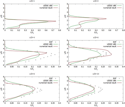
Thus, the obtained numerical results for the concentration component showed much better results than the obtained results using the LES turbulent model. Thus, the obtained values from the computation using the turbulent SST k-w model showed good agreement with the measured values and computational data for both the velocity components and the concentration components.

7. Test problem for a chemical reaction

To implement the test problem for a chemical reaction, a 2D model of a microreactor was constructed based on the data provided by Falconi et al. (2007). A similar work was done by foreign researchers (Schonauer & Adolph, 2005). The microreactor consisted of two channels. The diameter of the pipe (jet width) was D = 1 m, which was used as a unit of length. The height of the transverse channel 4D, the height of the pipe 2D, the length of the transverse channel 16D. The vertical channel was located precisely at the center of the vertical channel along the X-axis and was shifted by a range equal to 2.5D from the origin of the horizontal channel (Figure 15). Here the jet inlets from the pipe, perpendicular to the main flow in the channel. The flow conditions for the jet and the transverse flow were set by two various predetermined velocity profiles. Chemical component B inlets perpendicular to the flow (in 2), component A through the side channel (in 1). Figure 13 shows the configuration of the microreactor under study. Here, it was considered an incompressible fluid with $Re=\left(\right(\rho V_{\mathrm{\infty }}D\left)/\mu \right)=25$, where the chemical components A and B react and form a new substance C. ($A+B\stackrel{k}{\to }C$). The ratio of speeds was expressed through a coefficient $R=U_{jet}/U_{crossflow}=1.5$.

Figure 15. Scheme of the calculated area.

7.1. Initial and boundary conditions

Boundary conditions were determined like: the outlet – ‘Pressure-outlet’, the inlet 1 and inlet 2 – ‘Velocity-inlet’, the walls – ‘Wall’.

The velocity profile in the main channel was described as follows: $u_x=u_{wind}(1-e^{-5\zeta })$, where $\zeta =\text{min}(z,L_z-z)$. The remaining parameters were set constant: w = 0, $Y_A$ = 1, $Y_B$ = 0.

In the inlet pipe: u = 0, $w=2R{u}_{wind}(1-4r^2)$, where r = x, $Y_A$ = 0, $Y_B$ = 1. The remaining boundary conditions are specified as indicated in Table 1 and in Figure 16.

Figure 16. Numbering the outer boundaries of the solution domain.

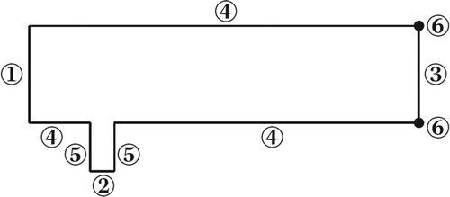
Table 1. Sequence of variables and equations at the boundaries of the $◯1$–$◯6$ domain.

Var.	$◯1$	$◯2$	$◯3$	$◯4$	$◯5$	$◯6$
u	$u_{wind}(1-e^{-5\zeta })$	u = 0	${\displaystyle \frac{\mathrm{\partial }u}{\mathrm{\partial }x}}=0$	u = 0	u = 0	u = 0
W	w = 0	Equation (1)	${\displaystyle \frac{\mathrm{\partial }w}{\mathrm{\partial }x}}=0$	w = 0	w = 0	w = 0
P	Equation (2)	p = $p_{atm}$	Equation (2)	Equation (2)	Equation (2)	Equation (2)
$Y_A$	$Y_A=0$	$Y_A=0$	${\displaystyle \frac{\mathrm{\partial }{Y}_A}{\mathrm{\partial }x}}=0$	${\displaystyle \frac{\mathrm{\partial }{Y}_A}{\mathrm{\partial }y}}=0$	${\displaystyle \frac{\mathrm{\partial }{Y}_A}{\mathrm{\partial }x}}=0$	${\displaystyle \frac{\mathrm{\partial }{Y}_A}{\mathrm{\partial }y}}=0$
$Y_B$	$Y_B=1$	$Y_B=1$	${\displaystyle \frac{\mathrm{\partial }{Y}_B}{\mathrm{\partial }x}}=0$	${\displaystyle \frac{\mathrm{\partial }{Y}_B}{\mathrm{\partial }y}}=0$	${\displaystyle \frac{\mathrm{\partial }{Y}_B}{\mathrm{\partial }x}}=0$	${\displaystyle \frac{\mathrm{\partial }{Y}_B}{\mathrm{\partial }y}}=0$

Here $u_{wind}$ varies depending on the selected substance. For substances A and B were indicated as oxygen O₂. For the numerical simulation of this problem, the following parameters were taken: the dynamic viscosity of oxygen was $\mu =1.919\times {10}^{-5}$ kg ${\text{m}}^2$/sec, density ρ = 1.299874 kg/${\text{m}}^3$, speed $u_{wind}=\text{0}\text{.000369074233}\text{m/s}$, hydraulic diameter D = 1 m, the diffusion coefficient was set, as 1.4762674052 m/${\text{s}}^2$. To satisfy the $Sc=1$, the diffusion coefficient was determined like $\text{0}\text{.677}{\text{m}}^{\text{2}}/s$. The rate of chemical reaction was taken as 1. In ANSYS Fluent, all calculations were made in actual sizes, so in this case the actual parameters were indicated.

7.2. A computational grid

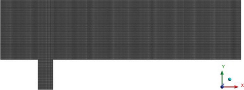
To obtain an accurate result, a structured computational grid was constructed. The main part of the channel consists of 641 × 141 computational points, the dimensions of the computational grid for the pipe are 41 × 81 and total the number of nodes is 638,886. The appreciate parameters for computational mesh generation is based on the computational data of Falconi et al. (2007) (Figure 17).

Figure 17. Calculate computational grid.

7.3. Comparison of computational values

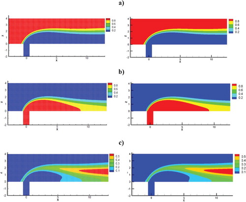
The computational values and a comparative analysis for the mass fraction and the velocity field are performed below. Values were matched with numerical values by Schonauer and Adolph (2005) and illustrated a good match. Figure 18 shows a comparison of the velocity streamlines with the computational values received by calculations of Schonauer and Adolph (2005). Figure 19 illustrates a comparative analysis of the velocity contour with the data from computations obtained by calculations of Schonauer and Adolph (2005) for horizontal velocity u and vertical velocity v. Figure 20 presents a comparative analysis of the of the concentrations distribution results obtained of this work and the results obtained by Falconi et al. (2007); Schonauer and Adolph (2005). As can be seen from the obtained data, the contours for the horizontal velocity u and the vertical velocity v showed good values in comparison with the calculations of Schonauer and Adolph (2005). The vortex length behind the pipe for both cases was l = 6.2D. It should also be noted that the distribution of the concentration component and the new concentration component also showed good agreement with numerical calculations (Schonauer & Adolph, 2005) (Figure 20).

Figure 18. The velocity streamlines comparison: the upper result is the calculations of Schonauer and Adolph (2005), the lower result is the obtained results in this work.

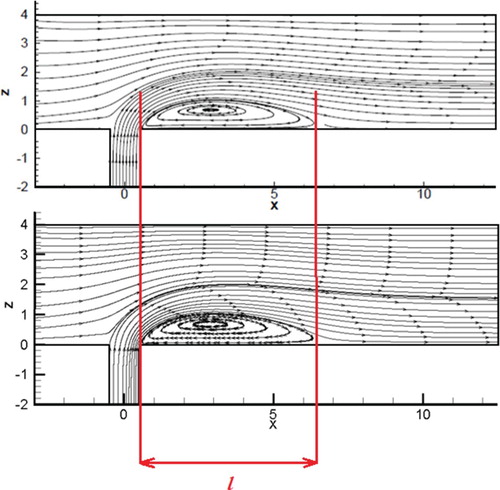
Figure 19. Comparative velocity contour analysis: left plots – results from Schonauer and Adolph (2005), the right-hand plots are the values obtained in the course of this work: (a) horizontal speed u (b) vertical speed v.

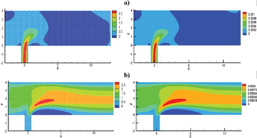
Figure 20. Comparative analysis of the results of the substance distribution: the left graphs – the values of Schonauer and Adolph (2005), the right-hand plots are the obtained results in this work: (a) concentration of substance A, (b) concentration of substance B, (c) concentration of substance C.

Thus, the obtained values from the computation using the turbulent SST k-w model showed good agreement with the measured values and computational data for both the velocity components, the concentration components and the concentration of product from the chemical reaction.

8. Real size problem

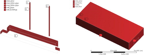
Next, the distribution of pollutants from Ekibastuz SDPP-1 in real sizes was considered (Figure 1). The computational domain is a 3D box with two chimneys inside it (Figure 21). At this Ekibastuz SDPP-1, pollution is produced from 2 chimneys, which have various altitudes of 300.0 and 330.0 m, respectively. The range between the two chimneys is 200.0 m (Figure 22). The diameters of the chimney holes are about 10.0 m. The NO, NO₂, CO, etc. are emitted in large quantities as pollutants from Ekibastuz SDPP-1. These pollutants in the atmosphere react with oxygen and water vapor. This paper discusses 3 major chemical reactions.

1. $2\text{CO}+{\text{O}}_2\to 2\text{C}{\text{O}}_2$

2. $2\text{NO}+{\text{O}}_2\to 2\text{N}{\text{O}}_2$

3. $4\text{N}{\text{O}}_2+2{\text{H}}_2\text{O}+{\text{O}}_2\to 4\text{HN}{\text{O}}_3$

Figure 21. Configuration of computing area for thermal power plant.

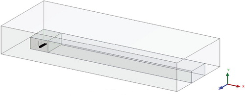
Figure 22. Parameters and dimensions of the calculated area.

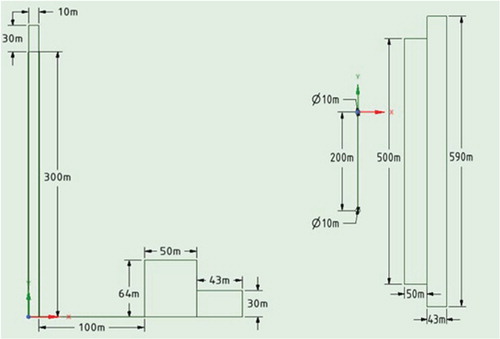
(1) The chemical reaction of carbon monoxide (CO) with oxygen produces carbon dioxide (CO₂) (carbon dioxide). Because of its toxicity, carbon monoxide is very dangerous for the human body. This danger is exacerbated by the fact that it is odorless and poisoning can occur unnoticed. Carbon monoxide interacts with blood hemoglobin (carboxyhemoglobin is formed), which is 200 times more active than oxygen and reduces the ability of blood to be its carrier. Therefore, even with low concentrations of CO in the air, it has a detrimental effect on health. When a chemical reaction with oxygen forms carbon dioxide. Carbon dioxide easily transmits radiation in the ultraviolet and visible parts of the spectrum, which comes to the earth from the sun and heats it. At the same time, it absorbs infrared radiation emitted by the earth and is one of the greenhouse gases, as a result of which it takes part in the process of global warming.

Besides the greenhouse properties of carbon dioxide, the fact that it is heavier than air is significant. Since the average relative molar mass of air is 28.98 g/mol and the molar mass of CO₂ is 44.01 g/mol, an increase in the proportion of carbon dioxide leads to an increase in air density and, accordingly, to a change in its pressure profile depending on height. Due to the physical nature of the greenhouse effect, such a change in the properties of the atmosphere leads to an increase in the average temperature on the surface (Stamler & Gow, 1998). Since, with an increase in the proportion of this gas in the atmosphere, its large molar mass leads to an increase in density and pressure, at the same temperature an increase in CO₂ concentration leads to an increase in the air capacity and to an increase in the greenhouse effect due to the large amount of water in the atmosphere. Increasing the proportion of water in the air to achieve the same level of relative humidity – due to the low molar mass of water (18 g/mol) – reduces the density of air, which compensates for the increase in density caused by the presence of elevated levels of carbon dioxide in the atmosphere.

(2) As a result of the chemical reaction of nitric oxide (NO) with oxygen, nitrogen dioxide (NO₂) is formed. Nitrogen oxide (II) is odorless, but when inhaled, it can bind to hemoglobin, like carbon monoxide gas converting it into a form (methemoglobin) that cannot transport oxygen (Stamler & Gow, 1998). Combined with oxygen in the air, it forms nitrogen dioxide. The NO₂ impurities paint industrial smokes brown. NO₂ irritates the lungs and can lead to serious health consequences. A concentration of NO₂ above 200 ppm is considered lethal, but already at a concentration above 60 ppm, discomfort and burning in the lungs can occur. NOx emissions are considered one of the main reasons for photochemical smog formation. Elevated concentrations of NOx have a detrimental effect on human health, therefore, standards have been adopted in various countries that limit the maximum allowable concentrations of NOx in the exhaust of power plants boilers, gas turbines, cars, airplanes and other devices. Improving combustion technologies is largely aimed at reducing NOx emissions while improving the energy efficiency of devices.

(3) As a result of the chemical reaction of nitrogen dioxide (NO₂) with oxygen and water vapor, nitric acid (HNO₃) is formed. As mentioned earlier, the resulting products are more harmful than the original. Nitric acid (HNO₃), together with sulfur oxides (SOx), is the cause of the formation of acid rain. Nitric acid is poisonous. According to the degree of impact on the body, it belongs to substances of the 3rd class of danger. It dissolves in fat and can penetrate into the capillaries of the lungs, where it causes inflammation and asthmatic processes, irritates the respiratory tract (Table 2).

Table 2. Parmameters of species.

	Parameters
Species	Density (kg/m^3)	Viscosity (w/m-K)	Cp (Specific Heat) (j/kg-K)	Thermal Conductivity (w/m-K)	Molecular Weight (kg/kmol)	Standard State Entropy (j/kgmol-K)
O2	1.2999	1.919 × 10^−5	piecewise-polynomial	0.0246	31.9988	205026.9
NO	1	1.72 × 10^−5	piecewise-polynomial	0.0454	30.0061	210640
NO2	1	1.72 × 10^−5	piecewise-polynomial	0.0454	46.0055	239909.6
H2O	0.5542	1.34 × 10^−5	piecewise-polynomial	0.0261	18.01534	188696.4
HNO3	1504	0.011	piecewise-polynomial	0.0454	63.01287	266389.2
Air	1.225	1.7894 × 10^−5	1006.43	0.0242	28.966	194336
CO	1.1233	1.75 × 10^−5	piecewise-polynomial	0.025	28.01055	197531.6
CO2	1.7878	1.37 × 10^−5	piecewise-polynomial	0.0145	44.00995	213720.2

8.1. Grid construction

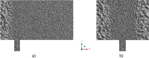
The computational grid was condensed in the area of the pollution trajectory, in which the area where the buildings are located (the size of the computational cell is up to 20 m) and then the concentration of the building (the size of the computational cell is up to 5 m) and the chimneys (the size of the computational cell is up to 2 m) (Figures 23–25). The computational grid consists of 218915 nodes and 1244098 elements (Table 3).

Figure 23. (a) computational grid and (b) bottom view of the grid.

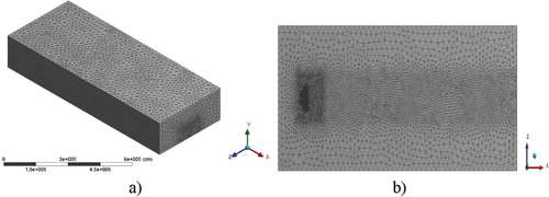
Figure 24. (a) section along the axis OXY and (b) section along the axis OYZ.

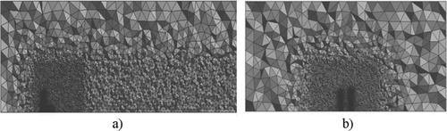
Figure 25. View of the chimneys and buildings.

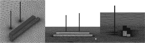
Table 3. Parmameters of geometry.

Geometry parameters (m)	First chimney coordinates (300 m)	Second chimney coordinates (330 m)
X = 10,000	X = 1000	X = 1000
Y = 1800	Y = 0	Y = 0
Z = 4000	Z = 2100	Z = 1900

8.2. Boundary conditions

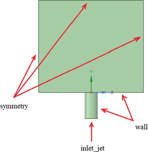
The boundary conditions were determined like: for the side walls and the top wall – the ‘Symmetry’, for the wind inlet and the chimney hole – the ‘Velocity inlet’, for the outlet – the ‘Pressure Outlet’ and for chimney walls, the ground – the ‘Wall’ (Figure 26).

Figure 26. Boundary conditions of the computational domain.

To represent the inlet velocity profile of the transverse flow the 1/7 power law of the wind in the boundary layer was used, as in Keimasi and Taeibi-Rahni (2001). The jet velocity was 1.5 m/s, the velocity of the transverse flow was 3 m/s. So the ratio of the jet velocity to the velocity of the transverse flow is R = 0.5. The ambient temperature is taken as 300 K. So the boundary conditions for the chimneys are taken as the concentration of different species like 1, and the concentration for different species of the transverse flow is taken as 0. And for all other domain sides are taken as no-flux boundary.

8.3. Numerical results

The numerical modeling was done in the ANSYS Fluent, where all modeling were performed in actual scales. For the computational solution SIMPLE approach was chosen.

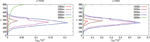
Figure 27 shows the concentration distribution of pollution, which is visualized using Volume Rendering. So Figure 27(a-d) displays the distribution of CO and CO₂ concentrations and for different angles of view. From Figure 27(e-h) one can see the spread of concentration for different angles of view. Figure 27(i-l) shows the distribution of concentration NO₂, HNO₃ for different angles of view. So from the obtained results it can be noted that the emitted concentrations and products from a chemical reaction extend very far. But it can also be noted that heavy elements obtained by a chemical reaction quickly precipitate near Ekibastuz SDPP-1. It can also be noted that with increasing distance from the source, a diffusion effect is observed for all kinds of concentration. Figures 28–30 show a comparison of the mass fraction profiles CO, CO₂, NO, NO₂, H₂O, NO₂, HNO₃ for different points: 1500, 2000, 2500, 3000, 10,000 and z = 2000.

Figure 27. Visualization of the spread of concentrations: (a-d) CO and CO₂, (e-h) NO and NO₂, (i-l) NO₂ and HNO₃.

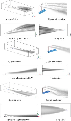
Figure 28. Comparison of profiles of the CO, CO₂ mass fractions in points: x = 1500, 2000, 2500, 3000, 10,000 and z = 2000.

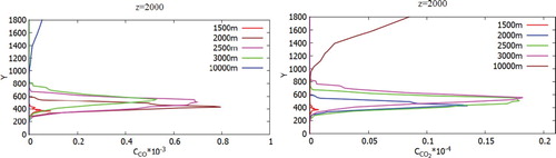
Figure 29. Comparison of profiles of the NO, NO₂ of mass fractions in points: 1500, 2000, 2500, 3000, 10,000 and z = 2000.

Figures 31–33 represent the comparison of the mass fractions of CO, NO, H₂O, NO₂ from two chimneys (300 and 330 m) at different distances at a wind speed of 3 m/s: 1000, 1500, 2500, 3000 and 10,000 m from the origin. As can be seen in the graphs, the mass fraction for a chimney with an altitude of 330 m is higher compared to a chimney of 300 m. Accordingly it can be concluded that the altitude of the chimneys essentially affects the contaminants spreading. Construction of higher chimney is more suitable for environmental safety.

Figure 30. Comparison of profiles of the H₂O, NO₂, HNO₃ mass fraction in points: 1500, 2000, 2500, 3000, 10,000 and z = 2000.

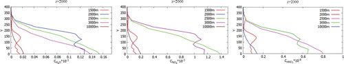
Figure 31. Comparison of profiles of the CO mass fraction at specified points for two various heights of chimneys (300.0 and 330.0 m).

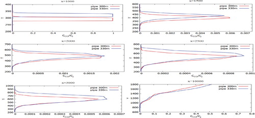
Figure 32. Comparison of profiles of the NO mass fraction at specified points for two various heights of chimneys (300.0 and 330.0 m).

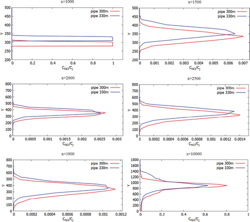
Figure 33. Comparison of profiles of the H₂O mass fraction at the specified points for two various heights of chimneys (300.0 and 330.0 m).

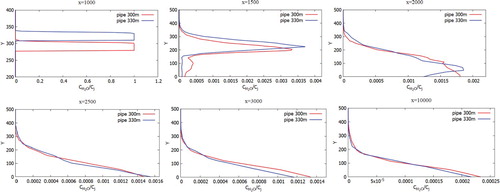
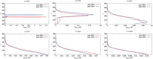
Figures 34–37 show the mass fractions of the products of a chemical reaction CO₂, NO₂, HNO₃ of two chimneys (300 and 330 m) compared at different distances at a wind speed of 3 m/s: 1000, 1500, 2500, 3000 and 10,000 m from the origin. From Figures 34–36 it can be noted that the pollutants do not immediately mix and enter into a chemical reaction, and the reaction process takes place through a certain distance from the chimneys. So active mixing starts from 500 m from the source. However, it should be noted that the concentration of CO and CO₂ practically does not have or has a very small value of concentration on the surface of the earth. This phenomenon is due to the fact that the density of CO is less than the density of air. And the concentration of CO₂, despite the fact that it matters more than the density of the air, could be explained by the fact that the impurity value CO₂ has a very small value. And also an important factor is that the formation of concentration CO₂ occurs around the distribution of CO. So from the data it can be concluded that the concentration of CO and CO₂ almost not deposited on the surface of the earth and goes down to about a height of 180 m.

Figure 34. Comparison of profiles of the CO₂ mass fraction at specified points for two various heights of chimneys (300.0 and 330.0 m).

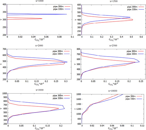
Figure 35. Comparison of profiles of the NO₂ mass fraction at specified points for two various heights of chimneys (300.0 and 330.0 m).

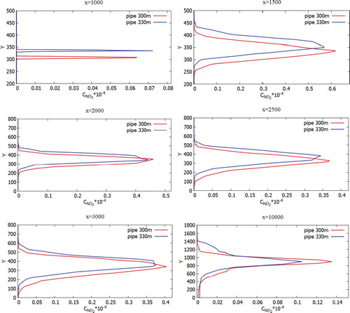
Figure 36. Comparison of profiles of the NO₂ mass fraction at the specified points for two various heights of chimneys (300.0 and 330.0 m).

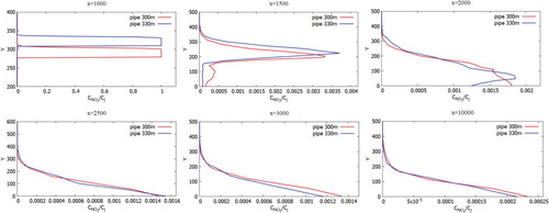
Figure 37. Comparison of profiles of the HNO₃ mass fraction at the specified points for two various heights of chimneys (300.0 and 330.0 m).

However, for the concentration of NO and NO₂ it can be noted that these concentrations descend a little below 100 m despite the fact that NO and NO₂ are lighter than air and than concentrations of CO and CO₂, this is due to the fact that these effects can be observed only in remote sections, since there is observed both the transfer process and the diffusion process. This process is due to turbulent vortex dissipation, which leads to the fact that the concentration of NO and NO₂ distributed in all directions evenly.

However, for concentration HNO₃, it can be seen the opposite situation, that most of the concentration settles on the ground surface and not too far from the Ekibastuz SDPP-1 chimney itself, and only a small part of the concentration HNO₃ remains on the atmospheric boundary layer. This rapid deposition of the most part HNO₃ could be explained that the density of the concentration HNO₃ is many times greater than the density of air. So from the obtained results it can be concluded that nitric acid (HNO₃) pollutes not only near the surface of the earth, but also the surface of the atmospheric layer. In the first case, the nearby territories of Ekibastuz SDPP-1 are polluted, and in the second case, a small part of the concentration of nitric acid (HNO₃) not only pollutes the air, but also lagging behind the small concentration in the atmosphere together with sulfur oxides (SOx) lead to cause and risk in the future the formation of acid rain.

In all the obtained pollution profiles, both the diffusion process and transfer process are seen. Because of the diffusion reason by turbulent vortex dissipation, the gas concentration sets to be higher at ground level by 20.0 m (where diffusion has smoother values). From the computational values, it could be noticed that the concentration rate that is releasing from two chimneys performs the significant role in the impurity distribution. Accordingly, having determined ground-based measurement points of concentrations CO₂, NO₂, HNO₃ in the regions, will be of significant interest in next study.

From the obtained computational values, it could also be noted that behind the chimneys as such, flow vortex regions of different sizes are not formed. Since with this movement of air, inertial forces predominantly prevail, which leads to the fact that the ejected concentration is not concentrated in the areas around the chimneys. And further from the chimneys, a clear dispersion of the allowed concentration is seen. So, in general, flow vortices of various sizes are visible in the concentration plume. Due to these processes, it can be seen from the results that the concentration of emissions is dissipated and expand downstream.

9. Conclusion

This paper presents the results obtained by numerical simulation using the software ANSYS FLUENT for the spread of pollutants formed during the combustion of fuel in an thermal power plant, and their chemical reaction in the atmosphere. The numerical method were tested using three test problems. Using several test problems for determination of the optimal turbulent model (k−ϵ and k–ω). Moreover, the analysis of the received computational values with the data of modeling other authors and measured data was done. As a result, the k – ω turbulent model was defined as the appreciate for the transfer to actual size problem.

Ekibastuz SDPP-1 was used to simulate an actual problem. A remarkable feature of this TPP is that the difference between the chimneys allows us to study the affect of the source height on the dispersion of pollution. The aim of the study was to study the dynamics of the emissions distribution and their chemical reaction with oxygen in the air. Using the example of a real thermal power plant, dispersions of CO, NO, H₂O, NO₂ and products CO₂, NO₂, HNO₃, were simulated during a chemical reaction with oxygen. From the values of the computation it can be concluded that the altitude of the chimneys essentially affects the gases spreading. In the analysis, it was found that it is necessary to simulate the process of locating a source that spreads harmful impurities from a TPP to the atmospheric boundary layer in such a way as to minimize air pollution and surrounding areas. The construction of higher chimneys for a TPP is most suitable for environmental safety.

It has to be noticed that in this work there are some limitations. The major limitation is the size of the computational grid. Computer resources are limited in the size of the computational grid, while a very huge computational grid is necessary to obtain an accurate simulation result. In addition, a further increase in computer resources will be followed by the requirements of researchers to increase the resolution of the grid and the extra physical parameters inclusion that will lead to actual size problem. The next limitation of the study is the complicacy of the analysis of computational studies on the distribution of chemical compounds in the atmosphere from the TPPs activities (size, shape, environmental factors). As well as the third limitation of this work is an accurate description of chemical reaction processes, since under real conditions the number of chemical reactions exceeds more than hundred reactions, and in modeling, a set of simplified chemical mechanisms is usually used to save computer resources. This work is useful for whose interested in the spreading of chemical compounds in the atmosphere from the TPPs activities.

Acknowledgements

This work is supported by grant from the Ministry of education and science of the Republic of Kazakhstan.

Disclosure statement

No potential conflict of interest was reported by the author(s).

Additional information

Funding

This work is supported by grant from the Ministry of Education and Science of the Republic of Kazakhstan.

References

- Ahmad, K., Khare, M., & Chaudhry, K. K. (2005). Wind tunnel simulation studies on dispersion at urban street canyons and intersections—a review. Journal of Wind Engineering and Industrial Aerodynamics, 93(9), 697–717. https://doi.org/10.1016/j.jweia.2005.04.002
- Ajersch, P., Zhou, J. M., Ketler, S., Salcudean, M., & Gartshore, I. S. (1995, June). Multiple jets in a cross flow: Detailed measurements and numerical simulations. In International gas turbine and aeroengine congress and exposition, ASME Paper 95-GT-9 (pp. 1–16). ASME.
- Akbarian, E., Najafi, B., Jafari, M., Faizollahzadeh Ardabili, S., Shamshirband, S., & Chau, K.-W. (2018). Experimental and computational fluid dynamics-based numerical simulation of using natural gas in a dual-fueled diesel engine. Engineering Applications of Computational Fluid Mechanics, 12(1), 517–534. https://doi.org/10.1080/19942060.2018.1472670
- Al-Abbas, A. H., Naser, J., & Dodds, D. (2011). CFD modelling of air-fired and oxy-fuel combustion of lignite in a 100 KW furnace. Fuel, 90(5), 1778–1795. https://doi.org/10.1016/%20j.fuel.2011.01.014
- Andersen, J., Rasmussen, C. L., Giselsson, T., & Glarborg, P. (2009, June 19–22). Global combustion mechanisms for use in CFD modeling under oxy-fuel conditions. Energy & Fuels, 23(3), 1379–1389. https://doi.org/10.1021/ef8003619
- Andersson, K., & Johnsson, F. (2006). Combustion and flame characteristics of oxy-fuel combustion-experimental activities within the Encap project. Proceedings of the GHGT-8 Conference, Trondheim, 2006.
- Andersson, K., & Johnsson, F. (2007). Flame and radiation characteristics of gas-fired O2/CO2 combustion. Fuel, 86(5-6), 656–668. https://doi.org/10.1016/j.fuel.2006.08.013
- Andreopoulos, J., & Rodi, W. (1984). Experimental investigation of jets in a crossflow. Journal of Fluid Mechanics, 138, 93–127. https://doi.org/10.1017/S0022112084000057
- Atkinson, R. (1989). Kinetics and mechanisms of the gas-phase reactions of the hydroxyl radical with organic compounds. Journal of Physical and Chemical Reference. Data, 1, 1–246. ISBN-10: 0883187205, ISBN-13: 978-0883187203
- Atkinson, R. (1990). Gas-phase tropospheric chemistry of organic compounds: A review. Atmospheric Environment. Part A. General Topics, 24(1), 1–41. https://doi.org/10.1016/0960-1686(90)90438-S
- Atkinson, R., & Carter, W. P. L. (1984). Kinetics and mechanisms of the gas-phase reactions of ozone with organic compounds under atmospheric conditions. Chemical Reviews, 84(5), 437–470. https://doi.org/10.1021/cr00063a002
- Atkinson, R., Hasegawa, D., & Aschmann, S. M. (1990a). Rate constants for the gas-phase reactions of O3 with a series of monoterpenes and related compounds at 296 ± 2 K. International Journal of Chemical Kinetics, 22(8), 871–887. https://doi.org/10.1002/kin.550220807
- Bahta, A., Simonaitis, R., & Heicklen, J. (1984). Reactions of ozone with olefins: Ethylene, allene, 1,3-butadiene, and trans-1,3-pentadiene. International Journal of Chemical Kinetics, 16(10), 1227–1246. https://doi.org/10.1002/kin.550161006
- Bennett, P. J., Harris, S. J., & Kerr, J. A. (1987). A reinvestigation of the rate constants for the reactions of ozone with cyclopentene and cyclohexene under atmospheric conditions. International Journal of Chemical Kinetics, 19(7), 609–614. https://doi.org/10.1002/kin.550190703
- Bloss, W. J. (2009). Atmospheric chemical processes of importance in cities. In R. M. Harrison & R. E. Hester (Eds.), Air quality in urban environments (pp. 42–64). The Royal Society of Chemistry.
- Bright, V. B., Bloss, W. J., & Cai, X. M. (2013). Urban street canyons: Coupling dynamics, chemistry and within-canyon chemical processing of emissions. Atmospheric Environment, 68, 127–142. https://doi.org/10.1016/j.atmosenv.2012.10.056
- Bulat, G., Jones, W. P., & Marquis, A. J. (2014). No and co formation in an industrial gas-turbine combustion chamber using LES with the Eulerian sub-grid PDF method. Combustion and Flame, 161(7), 1804–1825. https://doi.org/10.1016/j.combustflame.2013.12.028
- Chung, T. J. (2002). Computational fluid dynamics. Cambridge University Press. p. 1012.
- Crabb, D., Durao, D., & Whitelaw, J. (1981). A round jet normal to a crossflow. Transactions of the ASME: Journal of Fluids Engineering, 103(1), 568–580. https://doi.org/10.1115/1.3240764
- Denev, J. A., Fröhlich, J., & Bockhorn, H. (2006). Direct numerical simulation of mixing and chemical reactions in a round jet into a crossflow – a benchmark. In W. E. Nagel, W. Jaeger, & M. Resch (Eds.), Transaction of the high performance computing center Stuttgart (HLRS) 2006 (pp. 237–251). Springer.
- Ditaranto, M., & Oppelt, T. (2011). Radiative heat flux characteristics of methane flames in oxyfuel atmospheres. Experimental Thermal and Fluid Science, 35(7), 1343–1350. https://doi.org/10.1016/j.expthermflusci.2011.05.002
- Dunmore, R. E., Hopkins, J. R., Lidster, R. T., Lee, J. D., Evans, M. J., Rickard, A. R., Lewis, A. C., & Hamilton, J. F. (2015). Diesel-related hydrocarbons can dominate gas phase reactive carbon in megacities. Atmospheric Chemistry and Physics, 15(17), 9983–9996. https://doi.org/10.5194/acp-15-9983-2015
- Falconi, C. J., Denev, J. A., Frohlich, J., & Bockhorn, H. (2007). A test case for microreactor flows – a two-dimensional jet in crossflow with chemical reaction, Internal Report. “2d test case for microreactor flows. Internal report”. http://www.ict.uni-karlsruhe.de/index.pl/themen/dns/index.html.
- Ferziger, J. H., & Peric, M. (2013). Computational methods for fluid dynamics (3rd ed.). Springer. p. 426.
- Fiorina, B., Veynante, D., & Candel, S. (2015). Modeling combustion chemistry in large Eddy simulation of turbulent flames. Flow, Turbulence and Combustion, 94(1), 3–42. https://doi.org/10.1007/s10494-014-9579-8
- Frassoldati, A., Cuoci, A., & Faravelli, T. (2009). Simplified kinetic schemes for oxy-fuel combustion. In 1st International Conference of Sustain. Foss. Fuels Futur Energy (pp. 6–10).
- Ghalandari, M., Bornassi, S., Shamshirband, S., Mosavi, A., & Chau, K.-W. (2019). Investigation of Submerged Structures’ flexibility on Sloshing frequency using a boundary element method and finite element analysis. Engineering Applications of Computational Fluid Mechanics, 13(1), 519–528. https://doi.org/10.1080/19942060.2019.1619197
- Gillies, J. Z., Gillies, C. W., Suenram, R. D., & Lovas, F. J. (1988). The ozonolysis of ethylene: Microwave spectrum, molecular structure, and dipole moment of ethylene primary ozonide (1,2,3- trioxolane). Journal of the American Chemical Society, 110(24), 7991–7999. https://doi.org/10.1021/ja00232a007
- Goar, B. G. (1989, March 6–8). Emerging new sulfur technologies. Proceedings of the Laurance Reid Gas Conditioning Conference.
- Goar, B. G., & Hyne, J. B. (1996). Proceedings of the Laurance Reid Gas Conditioning Conference.
- Grosjean, D. (1990). Gas-phase reaction of ozone with 2-methyl-2-butene: Dicarbonyl formation from Criegee biradicals. Environmental Science & Technology, 24(9), 1428–1432. https://doi.org/10.1021/es00079a019
- Habib, M. A., Rashwan, S. S., Nemitallah, M. A., & Abdelhafez, A. (2017). Stability maps of non-premixed methane flames in different oxidizing environments of a gas turbine model combustor. Applied Energy, 189, 177–186. https://doi.org/10.1016/j.apenergy.2016.12.067
- Hatakeyama, S., & Akimoto, H. (1990). Reactions of ozone with 1-methylcyclohexene and methylenecyclohexane in air. Bulletin of the Chemical Society of Japan, 63(9), 2701–2703. https://doi.org/10.1246/bcsj.63.2701
- Herron, J. T., & Huie, R. E. (1978). Stopped-flow studies of the mechanisms of ozone-alkene reactions in the gas phase: Propene and isobutene. International Journal of Chemical Kinetics, 10(10), 1019–1041. https://doi.org/10.1002/kin.550101003
- Horie, O., & Moortgat, G. K. (1991). Decomposition pathways of the excited Criegee intermediates in the ozonolysis of simple alkenes. Atmospheric Environment Part A, 25, 1881–1896. https://doi.org/10.1016/0960-1686
- Issakhov, A. (2014). Modeling of synthetic turbulence generation in boundary layer by using Zonal RANS/LES method. International Journal of Nonlinear Sciences and Numerical Simulation, 15, 115–120. http://doi.org/10.1515/ijnsns-2012-0029
- Issakhov, A. (2016). Mathematical modeling of the discharged heat water effect on the aquatic environment from thermal power plant under various operational capacities. Applied Mathematical Modelling, 40(2), 1082–1096. https://doi.org/10.1016/j.apm.2015.06.024
- Issakhov, A., & Baitureyeva, A. (2019). Modeling of a passive scalar transport from thermal power plants to atmospheric boundary layer. International Journal of Environmental Science and Technology, 16(8), 4375–4392. https://doi.org/10.1007/s13762-019-02273-y
- Issakhov, A., Bulgakov, R., & Zhandaulet, Y. (2019a). Numerical simulation of the dynamics of particle motion with different sizes. Engineering Applications of Computational Fluid Mechanics, 13(1), 1–25. https://doi.org/10.1080/19942060.2018.1545253
- Issakhov, A., Bulgakov, R., & Zhandaulet, Y. (2019b). Numerical study of the dynamics of particles motion with different sizes from coal-based thermal power plant. International Journal of Nonlinear Sciences and Numerical Simulation, 20(2), 223–241. https://doi.org/10.1515/ijnsns-2018-0182
- Issakhov, A., & Imanberdiyeva, M. (2019). Numerical simulation of the movement of water surface of dam break flow by VOF methods for various obstacles. International Journal of Heat and Mass Transfer, 136, 1030–1051. https://doi.org/10.1016/j.ijheatmasstransfer.2019.03.034
- Issakhov, A., & Mashenkova, A. (2019). Numerical study for the assessment of pollutant dispersion from a thermal power plant under the different temperature regimes. International Journal of Environmental Science and Technology, 16(10), 6089–6112. https://doi.org/10.1007/s13762-019-02211-y
- Issakhov, A., & Omarova, P. (2020). Numerical simulation of pollutant dispersion in the residential areas with continuous grass barriers. International Journal of Environmental Science and Technology, 17(1), 525–540. https://doi.org/10.1007/s13762-019-02517-x
- Issakhov, A., Omarova, P., & Issakhov, A. (2020). Numerical study of thermal influence to pollutant dispersion in the idealized urban street road. Air Quality, Atmosphere & Health, https://doi.org/10.1007/s11869-020-00856-0
- Issakhov, A., & Zhandaulet, Y. (2019). Numerical simulation of thermal pollution zones’ formations in the water environment from the activities of the power plant. Engineering Applications of Computational Fluid Mechanics, 13(1), 279–299. https://doi.org/10.1080/19942060.2019.1584126
- Issakhov, A., & Zhandaulet, Y. (2020a). Numerical simulation of dam break waves on movable beds for various forms of the obstacle by VOF method. Water Resources Management, 34(8), 2269–2289. https://doi.org/10.1007/s11269-019-02480-9
- Issakhov, A., & Zhandaulet, Y. (2020b). Numerical study of dam break waves on movable beds for various forms of the obstacle by VOF method. Ocean Engineering, 209. Article 107459. https://doi.org/10.1016/j.oceaneng.2020.107459
- Issakhov, A., & Zhandaulet, Y. (2020c). Numerical study of technogenic thermal pollution zones’ formations in the water environment from the activities of the power plant. Environmental Modeling & Assessment, 25(2), 203–218. https://doi.org/10.1007/s10666-019-09668-8
- Issakhov, A., Zhandaulet, Y., & Nogaeva, A. (2018). Numerical simulation of dam break flow for various forms of the obstacle by VOF method. International Journal of Multiphase Flow, 109, 191–206. https://doi.org/10.1016/j.ijmultiphaseflow.2018.08.003
- Izumi, K., Murano, K., Mizuochi, M., & Fukuyama, T. (1988). Aerosol formation by the photooxidation of cyclohexene in the presence of nitrogen oxides. Environmental Science & Technology, 22(10), 1207–1215. https://doi.org/10.1021/es00175a014
- Jacobson, M. Z. (2005). Fundamentals of atmospheric modeling. Cambridge University Press.
- Keffer, J., & Baines, W. (1963). The round turbulent jet in a cross-wind. Journal of Fluid Mechanics, 15(4), 481–496. https://doi.org/10.1017/S0022112063000409
- Keimasi, R. M., & Taeibi-Rahni, M. (December 2001). Numerical simulation of Jets in a crossflow using different turbulence models. AIAA Journal, 39(39), 2268–2277. https://doi.org/10.2514/2.1264
- Kelso, R. M., Lim, T. T., & Perry, A. E. (1996). An experimental study of round jets in cross-flow. Journal of Fluid Mechanics, 306, 111–144. https://doi.org/10.1017/S0022112096001255
- Khalil, A. E. E., & Gupta, A. K. (2017a). Acoustic and heat release signatures for swirl assisted distributed combustion. Applied Energy, 193, 125–138. https://doi.org/10.1016/j.apenergy.2017.02.030
- Khalil, A. E. E., & Gupta, A. K. (2017b). Flame fluctuations in Oxy-CO2-methane mixtures in swirl assisted distributed combustion. Applied Energy, 204, 303–317. https://doi.org/10.1016/j.apenergy.2017.07.037
- Kikumoto, H., & Ooka, R. (2012). A numerical study of air pollutant dispersion with bimolecular chemical reactions in an urban street canyon using large-eddy simulation. Atmospheric Environment, 54, 456–464. https://doi.org/10.1016/j.atmosenv.2012.02.039
- Kim, H. K., Kim, Y., Lee, S. M., & Ahn, K. Y. (2007). Studies on combustion characteristics and flame length of turbulent oxy-fuel flames. Energy & Fuels, 21(3), 1459–1467. https://doi.org/10.1021/ef060346g
- Kim, M. J., Park, R. J., & Kim, J.-J. (2012). Urban air quality modeling with full O3–NOx–VOC chemistry: Implications for O3 and PM air quality in a street canyon. Atmospheric Environment, 47, 330–340. https://doi.org/10.1016/j.atmosenv.2011.10.059
- Kwak, K. H., Baik, J. J., & Lee, K. Y. (2013). Dispersion and photochemical evolution of reactive pollutants in street canyons. Atmospheric Environment, 70, 98–107. https://doi.org/10.1016/j.atmosenv.2013.01.010
- Launder, B. E., & Spalding, D. B. (1974). The numerical computation of turbulent flows. Computer Methods in Applied Mechanics and Engineering, 3(2), 269–289. https://doi.org/10.1016/0045-7825(74)90029-2
- Li, X. X., Britter, R. E., Norford, L. K., Koh, T. Y., & Entekhabi, D. (2012). Flow and pollutant transport in urban street canyons of different aspect ratios with ground heating: Large-eddy simulation. Boundary-Layer Meteorology, 142(2), 289–304. https://doi.org/10.1007/s10546-011-9670-9
- Li, X.-X., Leung, D. Y. C., Liu, C.-H., & Lam, K. M. (2008a). Physical modeling of flow field inside urban street canyons. Journal of Applied Meteorology and Climatology, 47(7), 2058–2067. https://doi.org/10.1175/2007JAMC1815.1
- Li, Y., Li, H., Guo, H., Li, Y., & Yao, M. (2018). A numerical investigation on NO2 formation in a natural gas–diesel dual fuel engine. Journal of Engineering for Gas Turbines and Power, 140(9), 092804. https://doi.org/10.1115/1.4039734
- Li, X.-X., Liu, C.-H., & Leung, D. Y. C. (2008b). Large-eddy simulation of flow and pollutant dispersion in high-aspect-ratio urban street canyons with wall model. Boundary-Layer Meteorology, 129(2), 249–268. https://doi.org/10.1007/s10546-008-9313-y
- Li, B., Shi, B., Zhao, X., Ma, K., Xie, D., Zhao, D., & Li, J. (2018). Oxy-fuel combustion of methane in a swirl tubular flame burner under various oxygen contents: Operation limits and combustion instability. Experimental Thermal and Fluid Science, 90, 115–124. https://doi.org/10.1016/j.expthermflusci.2017.09.001
- Li, Z., Xu, H., Yang, W., Xu, M., & Zhao, F. (2019). Numerical investigation and thermodynamic analysis of syngas production through chemical looping gasification using biomass as fuel. Fuel, 246, 466–475. https://doi.org/10.1016/j.fuel.2019.03.007
- Liu, G., Liao, Y., Wu, Y., Ma, X., & Chen, L. (2017). Characteristics of microalgae gasification through chemical looping in the presence of steam. International Journal of Hydrogen Energy, 42(36), 22730–22742. https://doi.org/10.1016/j.ijhydene.2017.07.173
- Maddox, R. N. (1998). Gas conditioning and processing: gas and liquid sweetening. Campbell petroleum series.
- Majander, P., & Siikonen, T. (2006). Large-eddy simulation of a round jet in a cross-flow. International Journal of Heat and Fluid Flow, 27(3), 402–415. https://doi.org/10.1016/j.ijheatfluidflow.2006.01.004
- Martinez, R. I., & Herron, J. T. (1988). Stopped-flow studies of the mechanisms of ozone-alkene reactions in the gas-phase: Trans-2- Butene. The Journal of Physical Chemistry, 92(16), 4644–4648. https://doi.org/10.1021/j100327a017
- Martinez, R. I., Herron, J. T., & Huie, R. E. (1981). The mechanism of ozone-alkene reactions in the gas phase: A mass spectrometric study of the reactions of eight linear and branched-chain alkenes. Journal of the American Chemical Society, 103(13), 3807–3820. https://doi.org/10.1021/ja00403a031
- Mărunţălu, O., Lăzăroiu, G., Manea, E., Bondrea, D., & Robescu, L. (2015). Numerical simulation of the air pollutants dispersion emitted by CHP using ANSYS CFX. World Academy of Science, Engineering and Technology, International Journal of Environmental, Chemical, Ecological, Geological and Geophysical Engineering, 9(9), 951–957. http://doi.org/10.5281/zenodo.1108252
- Mayer, H. (1999). Air pollution in cities. Atmospheric Environment, 33(24-25), 4029–4037. https://doi.org/10.1016/S1352-2310(99)00144-2
- Menter, F. R. (1993). Zonal two equation k-ω turbulence models for aerodynamic flows. AIAA Paper, 93–2906. https://doi.org/10.2514/6.1993-2906
- Menter, F. R. (1994). Two-equation eddy-viscosity turbulence models for engineering applications. AIAA Journal, 32(8), 1598–1605. https://doi.org/10.2514/3.12149
- Mou, B., He, B.-J., Zhao, D.-X., & Chau, K.-W. (2017). Numerical simulation of the effects of building dimensional variation on wind pressure distribution. Engineering Applications of Computational Fluid Mechanics, 11(1), 293–309. https://doi.org/10.1080/19942060.2017.1281845
- Muhammad, N., Nadeem, S., & Issakhov, A. (2020). Finite volume method for mixed convection flow of Ag–ethylene glycol nanofluid flow in a cavity having thin central heater. Physica A: Statistical Mechanics and its Applications, 537. Article 122738. https://doi.org/10.1016/j.physa.2019.122738
- Muñoz, V., Casado, C., Suárez, S., Sánchez, B., & Marugán, J. (2018). Photocatalytic NOx removal: Rigorous kinetic modelling and ISO standard reactor simulation. Catalysis Today, https://doi.org/10.1016/j.cattod.2018.09.001
- Muppidi, S., & Mahesh, K. (1999). Study of trajectories of jets in crossflow using direct numerical simulations. Journal of Fluid Mechanics, 530, 81–100. https://doi.org/10.1017/S0022112005003514
- Muppidi, S., & Mahesh, K. (2008). Direct numerical simulation of passive scalar transport in transverse jets. Journal of Fluid Mechanics, 598, 335–360. https://doi.org/10.1017/S0022112007000055
- Niki, H., Maker, P. D., Savage, C. M., & Breitenbach, L. P. (1983). Atmospheric ozone-olefin reactions. Environmental Science & Technology, 17(7), 312A–322A. https://doi.org/10.1021/es00113a720
- Niki, H., Maker, P. D., Savage, C. M., Breitenbach, L. P., & Hurley, M. D. (1987). FTIR spectroscopic study of the mechanism for the gas-phase reaction between ozone and tetramethylethylene. The Journal of Physical Chemistry, 91(4), 941–946. https://doi.org/10.1021/j100288a035
- Nolting, F., Behnke, W., & Zetzsch, C. (1988). A smog chamber for studies of the reactions of terpenes and alkanes with ozone and OH. Journal of Atmospheric Chemistry, 6(1-2), 47–59. https://doi.org/10.1007/BF00048331
- Patankar, S. V. (1980). Numerical heat transfer and fluid flow. Taylor & Francis.
- Paulson, S. E., Flagan, R. C., & Seinfeld, J. H. (1992). Atmospheric photooxidation of isoprene part II: The ozone-isoprene reaction. International Journal of Chemical Kinetics, 24(1), 103–125. https://doi.org/10.1002/kin.550240110
- Salim, S. M., Buccolieri, R., Chan, A., & Di sabatino, S. (2011). Numerical simulation of atmospheric pollutant dispersion in an urban street canyon: Comparison between RANS and LES. Journal of Wind Engineering and Industrial Aerodynamics, 99(2-3), 103–113. https://doi.org/10.1016/j.jweia.2010.12.002
- Schonauer, W., & Adolph, T. (2005). FDEM: The evolution and application of the finite difference element method (FDEM) program package for the solution of partial differential equations, Abschlussbericht des Verbundprojekts FDEM, Universitä Karlsruhe. http://www.rz.uni-karlsruhe.de/rz/docs/FDEM/Literatur/fdem.pdf.
- Sherif, S. A., & Pletcher, R. H. (June 1989). Measurements of the flow and turbulence characteristics of round jets in crossflow. Journal of Fluids Engineering, 111(2), 165–171. https://doi.org/10.1115/1.3243618
- Shi, S., Guenther, C., & Orsino, S. (2007). Numerical study of coal gasification using Eulerian-Eulerian Multiphase model. ASME 2007 power Conference. https://doi.org/10.1115/power2007-22144
- Shi, S.-P., Zitney, S. E., Shahnam, M., Syamlal, M., & Rogers, W. A. (2006). Modelling coal gasification with CFD and discrete phase method. Journal of the Energy Institute, 79(4), 217–221. https://doi.org/10.1179/174602206x148865
- Shorees, B., Atkinson, R., & Arey, J. (1991). Kinetics of the gas-phase reactions of/3-phellandrene with OH and NO 3 radicals and 03 at 297. 2 K. International Journal of Chemical Kinetics, 23(10), 897–906. https://doi.org/10.1002/kin.550231005
- Smith, G. P., Golden, D. M., Frenklach, M., Moriarty, N. W., Eiteneer, B., Goldenberg, M., Bowman, C. T., Hanson, R. K., Song, S., Gardiner, W. C., Lissianski, V. V., & Qin, Z. (1999). GRI-Mech 3.0. 51:55. http://www.me.berkeley.edu/gri-mech.
- Stamler, J. S., & Gow, A. J. (1998). Reactions between nitric oxide and haemoglobin under physiological conditions. Nature, 391(6663), 169–173. https://doi.org/10.1038/34402
- U.S. Environmental Protection Agency. Clean air markets division. https://ampd.epa.gov/ampd/
- Vardoulakis, S., Fisher, B. E. A., Pericleous, K., & Gonzalez-flesca, N. (2003). Modelling air quality in street canyons: A review. Atmospheric Environment, 37(2), 155–182. https://doi.org/10.1016/S1352-2310(02)00857-9
- Versteeg, H. K., & Malalasekera, W. (1996). An introduction to computational fluid dynamics—the finite volume method, Logman Malaysia, reprinted, Chaps. 5–7.
- Wegner, B., Huai, Y., & Sadiki, A. (2004). Comparative study of turbulent mixing in jet in cross-flow configurations using les. International Journal of Heat and Fluid Flow, 25(5), 767–775. https://doi.org/10.1016/j.ijheatfluidflow.2004.05.015
- Wu, Z., & Liu, C.-H. (2018). Budget analysis for reactive plume transport over idealised urban areas. Geoscience Letters, 5(1), https://doi.org/10.1186/s40562-018-0118-7
- Yazid, A. W. M., Sidik, N. A. C., Salim, S. M., & Saqr, K. M. (2014). A review on the flow structure and pollutant dispersion in urban street canyons for urban planning strategies. Simulation, 90(8), 892–916. https://doi.org/10.1177/0037549714528046
- Yokouchi, Y., & Ambe, Y. (1985). Aerosols formed from the chemical reaction of monoterpenes and ozone. Atmospheric Environment (1967), 19(8), 1271–1276. https://doi.org/10.1016/0004-6981(85)90257-4
- Yuan, L. L., Street, R. L., & Ferziger, J. H. (1999). Large-eddy simulations of a round jet in crossflow. Journal of Fluid Mechanics, 379, 71–104. https://doi.org/10.1017/S0022112098003346
- Zhong, J., Cai, X.-M., & Bloss, W. J. (2015). Modelling the dispersion and transport of reactive pollutants in a deep urban street canyon: Using large-eddy simulation. Environmental Pollution, 200, 42–52. https://doi.org/10.1016/j.envpol.2015.02.009
- Zhong, J., Cai, X.-M., & Bloss, W. J. (2016). Coupling dynamics and chemistry in the air pollution modelling of street canyons: A review. Environmental Pollution, 214, 690–704. https://doi.org/10.1016/j.envpol.2016.04.052
- Ziefle, J., & Kleiser, L. (2009). Large-Eddy simulation of a round jet in crossflow. AIAA Journal, 47(5), 1158–1172. https://doi.org/10.2514/1.38465
- Zozom, J., Gillies, C. W., Suenram, R. D., & Lovas, F. J. (August 1987). Microwave detection of the primary ozonide of ethylene in the gas phase. Chemical Physics Letters, 140(1), 64–70. https://doi.org/10.1016/0009-2614(87)80418-9