Coupling analysis of transient aerodynamic and dynamic response of cars in overtaking under crosswinds

Abstract

The aerodynamic performance and dynamic response of two cars in overtaking maneuver under crosswind were investigated using a multi-car two-way coupling method. The coupling was achieved by exchanging aerodynamic forces obtained by computational fluid dynamic and vehicle dynamic responses acquired by multi-body dynamics in real time. The change rules of the aerodynamic force, moment, yaw angle, and lateral displacement of overtaking and overtaken cars were revealed on the basis of coupling computation. The coupling effect between aerodynamics and dynamics and the interplay between overtaking and overtaken cars were also illustrated. Moreover, the necessity of the two-way coupling was verified. Final results indicated that the posture of the body and the lateral space of the two vehicles are crucial to the stability of the vehicles during the overtaking maneuver, and the interaction between the aerodynamic forces and the dynamic response should be considered.

KEYWORDS:

• Multi-car two-way coupling
• vehicle dynamics
• transient aerodynamics
• multi-body dynamics
• overtaking

1. Introduction

As one vehicle passes another during an overtaking maneuver in crosswinds at high speed, the transient aerodynamic forces are generated due to changes in the flow fields around the two vehicles. The additional aerodynamic forces acting on the vehicle may induce sudden lateral displacements and yaw velocity, thereby adversely affecting vehicle handling stability, and even safety. Meanwhile, the deteriorative dynamic response will further influence the aerodynamic performance of vehicles. Self-driving and active safety technologies have been receiving increasing attention, but sudden changes in lateral displacements and yaw velocity will complicate the path correction or even cause loss of control. Therefore, revealing the aerodynamic characteristics and dynamic response of vehicles during overtaking maneuvers under crosswinds is important.

Early studies related to the aerodynamic performance of vehicles in overtaking were conducted by wind tunnel tests. For instance, the effects of the longitudinal and lateral space between two vehicles on the aerodynamic characteristics during overtaking maneuver were revealed by a 1/10 scale model (Azim, 1994). A car–truck overtaking wind tunnel test indicated that the pressure field around the front of a truck greatly influences the forces experienced by the overtaking car, and the influence is mainly dependent on the truck velocity. The dynamic changes in the side force and the yaw moment are also important concerns (Howell et al., 2014; Noger & Grevenynghe, 2011). A further wind tunnel test also revealed the influence of velocity ratio between the two overtaking vehicles on their aerodynamic performance (Telionis et al., 1984; Yamamoto et al., 1997). However, in the traditional wind tunnel, the tests are steady, thereby concealing the transient characteristics. Moreover, the wind tunnel test is costly and difficult to evaluate the aerodynamic performance of vehicles under complex environments in the early stages of vehicle development.

With the development of computational fluid dynamics (CFD) and high-performance computers, numerical simulation has been used to reveal the aerodynamic characteristics of vehicles in overtaking. Quasi-static computational methods were traditionally applied to analyse the aerodynamic performance of two vehicles in various relative positions during the overtaking maneuver (Gu, 2008; Sun et al., 2019). These studies showed that the force and the yaw moment change remarkably as the overtaking vehicle moves from the rear of the overtaken vehicle to the front. Meanwhile, a computational method using a discontinuous interface grid and moving boundaries was developed to analyze the transient aerodynamic phenomenon (Clarke & Filippone, 2007; Liu et al., 2018; Okumura & Kuriyama, 2010; Uystepruyst & Krajnović, 2013). The results showed that the yaw moment experienced by an overtaken car is almost twice than that obtained by the quasi-static computation, and the increase in the relative velocity or acceleration of the two cars and the reduction in lateral space will increase the aerodynamic forces acting on the car. Invariably, the vehicle's path in overtaking are predetermined and the dynamic responses, such as the changes in yaw velocity, lateral displacement and body posture, are ignored in the above-mentioned research. However, the amplitude and direction of the aerodynamic forces on vehicles will be changed constantly with changes in yaw velocity, lateral displacement even body posture so that the movement of the vehicle during overtaking maneuver will be inevitably affected further. Meanwhile, the aerodynamic performance will be influenced by the dynamic response again. Therefore, considering the interaction between the dynamic response and aerodynamic in overtaking is necessary. Moreover, in traditional numerical simulation about the overtaking, the overtaken vehicles were assumed to be stationary with a relative velocity added to the overtaking vehicle, and the dynamic response and the change in the aerodynamic forces of the overtaken vehicle were not considered. However, the aerodynamic characteristics and movement of the overtaken vehicle are severely affected by overtaking maneuver especially in sedan–sedan overtaking(Liu et al., 2018). Conversely, the change in the aerodynamic forces and dynamic response of the overtaken vehicle will further influence the overtaking vehicle. Therefore, simultaneously maintaining the dynamic movement of the two vehicles in the overtaking maneuver is necessary to accurately capture the aerodynamic characteristics and dynamic response changes.

In view of the importance of the dynamic response to the aerodynamic performance, considerable attention has recently been provided to the interaction between aerodynamics and motions of vehicle in overtaking. Initially, the one-way coupling method, where the aerodynamic forces are exerted to the dynamic model to obtain the response, was proposed. For instance, Nakashima et al. (Nakashima et al., 2010; Nakashima et al., 2011) investigated the aerodynamic performance of a heavy-duty truck in sudden crosswinds by coupling a three-degrees-of-freedom or six-degrees-of-freedom vehicle dynamic model with an aerodynamics model. Lewington et al.(Lewington et al., 2017) and (Zhang et al., 2020) applied the output of aerodynamic forces and moments from a CFD model directly to a multi-body dynamics (MBD) model to compute the dynamic response of the vehicle in crosswind. In the one-way coupling method, unlike the predetermined motion in the quasi-static method, the motion locus could be obtained by the dynamic model. However, the aerodynamic inputs to the dynamic model remained quasi-static. Thus, the influence of the dynamic responses of the vehicles on the aerodynamic performance was not considered. The one-way coupling method cannot update vehicle motion in real time to truly capture the changes in vehicle aerodynamic forces.

Hence, a two-way coupling method, which can compute the interaction between aerodynamic and vehicle dynamic response accurately, is proposed by Nakashima et al. (Nakashima et al., 2013). The results clearly demonstrated the necessity of considering transient aerodynamic forces in dynamic response analysis. The real-time dynamic response and aerodynamic forces could be computed by the kinetics model and the aerodynamic model by using the two-way coupling method (Nakasato et al., 2017; Winkler et al., 2016; Wang et al. 2020; Zhang et al. 2020). At present, this approach has been used to analyse the aerodynamic performance and dynamic response of the vehicle in crosswinds (Huang et al., 2018; Li et al., 2018). The results demonstrated that the influence of the aerodynamic forces on the vehicle motion in the two-way coupling method is greater than that in the one-way coupling method.

The coupling effect between aerodynamics and dynamics during overtaking will influence the aerodynamic characteristics and dynamic response of two cars. Therefore, in current research, a multi-cars two-way coupling method was developed to investigate the aerodynamic characteristics and dynamic response of vehicles during overtaking maneuver under crosswinds. The absolute velocity, rather than the relative velocity, was imposed to vehicles to obtain the aerodynamic performance and dynamic response of the overtaken vehicle and improve the applicability of the numerical simulation. The necessary of coupling analysis of aerodynamic and dynamic response during the overtaking is demonstrated by comparing the results obtained by the uncoupling approach. Finally, the aerodynamic characteristics and dynamic response of the overtaking and overtaken cars during overtaking under crosswinds are revealed.

2. Methodology

A schematic diagram of the two-way coupling method performed in current research is plotted in Figure 1. The computational platform is constructed by coupling CFD commercial solver Ansys Fluent with MBD commercial solver MSC ADAMS. Meanwhile, an interface program was compiled to achieve the data exchange between the two solvers in real time. The aerodynamic forces computed by the CFD model were sent to the MBD model, and the dynamic responses computed by the MBD were fed back to the CFD model.

Figure 1. Coupling system of CFD and MBD.

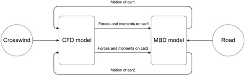
Moreover, given that the location of the wind pressure center is not constant in time and space, a reference point for computing the aerodynamic forces must be defined. The aerodynamic force acted at the center of the pressure can be equivalent to the force and moment acted at the reference point. In current research, the reference point was positioned at the center of the four wheel hubs. The aerodynamic forces in the MBD model were also applied to the reference point.

2.1. Governing equations for aerodynamic load computation

The flow field around the sedan during overtaking is three-dimensional, non-stationary, turbulent and incompressible. The mass and momentum conservation equations are solved by Fluent using the Reynolds-averaged Navier-Stokes equations in general non-steady coordinates system ${\xi }^j$ (Margot et al., 2010; Salih et al., 2019; Warsi, 1981).

The continuity conservation equation is: (1) $\frac{\mathrm{\partial }}{\mathrm{\partial }{\xi }^j}(\overline{u_{mj}})=0$(1)

The momentum conservation equation is: (2) $\frac{\mathrm{\partial }\overline{u_i}}{\mathrm{\partial }t}+\frac{\mathrm{\partial }(\overline{u_{mj}}\overline{u_i})}{\mathrm{\partial }{\xi }^j}=-\frac{1}{\rho }\frac{\mathrm{\partial }\overline{P}}{\mathrm{\partial }{\xi }^j}+\frac{1}{\rho }\frac{\mathrm{\partial }}{\mathrm{\partial }{\xi }^j}\left(\mu \frac{\mathrm{\partial }\overline{u_i}}{\mathrm{\partial }{\xi }^j}-\rho \overline{{u_i}^{\mathrm{\prime }}{u_j}^{\mathrm{\prime }}}\right)$(2) where the overbar indicates the Reynolds average, ${\xi }^i$ is the non-steady coordinates system (i = 1, 2, 3), ρ is the fluid density, P is the pressure, ${u_i}^{\mathrm{\prime }}$ is the fluctuations of the velocity, t is time, $u_i$ is the absolute fluid velocity component in direction ${\xi }^i$, $u_{mj}=u_j-u_{gj}$ is the relative velocity between the fluid velocity $u_j$ and the grid moving velocity $u_{gj}$, and $-\overline{{u_i}^{\mathrm{\prime }}{u_j}^{\mathrm{\prime }}}$ is the Reynolds-stress tensor, which is modeled by the Boussinesq assumption. (3) $-\overline{{u_i}^{\mathrm{\prime }}{u_j}^{\mathrm{\prime }}}=v_t\left(\frac{\mathrm{\partial }{u}_i}{\mathrm{\partial }{x}_j}+\frac{\mathrm{\partial }{u}_j}{\mathrm{\partial }{x}_i}\right)-\frac{2}{3}{\delta }_{ij}k$(3) where $v_t$ is the turbulence kinematic viscosity and $k$ is the turbulence kinetic energy. (4) $k=\frac{1}{2}\overline{{u_i}^{\mathrm{\prime }}{u_i}^{\mathrm{\prime }}}$(4)

To make the aforementioned conservation equations be closure, the $k-\epsilon$ turbulence model is widely employed, e.g. standard $k-\epsilon$ model (Akbarian et al., 2018; Blocken & Toparlar, 2015), and RNG $k-\epsilon$ model (Clarke & Filippone, 2007; Wang & Hu, 2012). Considering the good overall performance to predict vortices on the windward and leeward sides (Koutsourakis et al., 2012) and computational accuracy, a three-dimensional, incompressible, unsteady RNG $k-\epsilon$ two-equation turbulent model is utilized. The turbulent kinetic energy dissipation rate $\epsilon$ are determined by: (5) $\begin{array}{rl}& \frac{\mathrm{\partial }}{\mathrm{\partial }t}(\rho k)+\frac{\mathrm{\partial }}{\mathrm{\partial }{x}_i}(\rho k{u}_i)\\ & =\frac{\mathrm{\partial }}{\mathrm{\partial }{x}_j}\left({\alpha }_k{\mu }_{eff}\frac{\mathrm{\partial }k}{\mathrm{\partial }{x}_i}\right)+G_k+G_b-\rho \epsilon \end{array}$(5) (6) $\begin{array}{rl}& \frac{\mathrm{\partial }}{\mathrm{\partial }t}(\rho \epsilon )+\frac{\mathrm{\partial }}{\mathrm{\partial }{x}_i}(\rho \epsilon u_i)\\ & =\frac{\mathrm{\partial }}{\mathrm{\partial }{x}_j}\left({\alpha }_{\epsilon }{\mu }_{eff}\frac{\mathrm{\partial }\epsilon }{\mathrm{\partial }{x}_j}\right)+C_{1\epsilon }\frac{\epsilon }{k}(G_k+C_{3\epsilon }{G}_b)\\ & -C_{2\epsilon }\rho \frac{{\epsilon }^2}{k}-R_{\epsilon }\end{array}$(6) where $G_k$ is the turbulent flow energy from the laminar velocity gradient, and $G_b$ is the turbulent flow energy from buoyancy. Additional details about the governing equations can be found in the reference (Yakhot & Orszag, 1986).

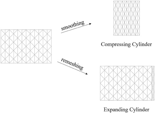
Generally, to enable the motion of the vehicles, the dynamic mesh technology is often employed (Salati et al., 2018). For the dynamic mesh model, the mesh is adjusted according to the movement of the region boundaries, and the mesh is automatically updated according to the position of the boundaries. At present, there are several strategies for the mesh update in dynamic mesh technology (Du et al., 2010). In current research, the smoothing method and the re-meshing technique were used to update the grids in the moving area according to the movement of the boundaries (Fluent, 2009), as shown in Figure 2. The smoothing method was used for a small movement of the boundary. The topology of the mesh does not change when the interior nodes move. Thus, the interior nodes absorb the movement of the boundary. When the boundary displacement exceeds certain value, the qualities of some of the morphed cells may be detreated to an unacceptable level. The re-meshing technique was adopted to re-mesh the agglomerated cells or faces which do not meet the criteria of the skewness or size locally.

Figure 2. Two methods of mesh motion.

For a scalar in dynamic mesh, the equation can be written as follows:: (7) $\begin{array}{rl}& \frac{d}{dt}{\int }_V\rho \varphi dV+{\int }_{\mathrm{\partial }V}\rho \varphi (\overrightarrow{u}-{\overrightarrow{u}}_g)\cdot d\overrightarrow{A}\\ & ={\int }_{\mathrm{\partial }V}\mathrm{\Gamma }\mathrm{\nabla }\varphi \cdot d\overrightarrow{A}+{\int }_V{S}_{\varphi }dV\end{array}$(7) where $\overrightarrow{u}$ is the flow velocity, ${\overrightarrow{u}}_g$ is the moving velocity of the sedan, which is obtained from multi-body dynamics calculations, $\mathrm{\Gamma }$ is the diffusion coefficient, $S_{\varphi }$ is the source term of $\varphi$, and $\mathrm{\partial }V$ denote surface area vector and the boundary of the control volume $V$ respectively.

The time derivative in Equation (7) can be written as: (8) $\frac{d}{dt}{\int }_V\rho \varphi dV=\frac{3{(\rho \varphi V)}^{n+1}-4{(\rho \varphi V)}^n+{(\rho \varphi V)}^{n-1}}{2\mathrm{\Delta }t}$(8) where n+1, n, n-1 are successive time levels, $V^{n+1}$ is the (n+1)th time level volume. (9) $\begin{array}{rl}{V}^{n+1}& =V^n+\frac{dV}{dt}\mathrm{\Delta }t\end{array}$(9) (10) $\begin{array}{rl}\frac{dV}{dt}& ={\int }_{\mathrm{\partial }V}\overrightarrow{u_g}\cdot d\overrightarrow{A}=\sum _j^{n_f}\overrightarrow{u_{g,j}}\cdot \overrightarrow{A_j}\end{array}$(10) The dot product on each face is calculated by: (11) $\begin{array}{rl}(\overrightarrow{u_{g,j}}\cdot \overrightarrow{A_j}{)}^{n+1}& =\frac{3}{2}(\overrightarrow{u_{g,j}}\cdot \overrightarrow{A_j}{)}^n-\frac{1}{2}(\overrightarrow{u_{g,j}}\cdot \overrightarrow{A_j}{)}^{n-1}\\ & =\frac{3}{2}{\left(\frac{\delta V_j}{\mathrm{\Delta }t}\right)}^n-\frac{1}{2}{\left(\frac{\delta V_j}{\mathrm{\Delta }t}\right)}^{n-1}\end{array}$(11) where $(\delta V_j{)}^n$ and $(\delta V_j{)}^{n\text{ - }1}$ are the volumes swept out by control volume faces at two adjacent time levels.

2.2. Governing equations for dynamic response

The multi-body dynamic model used to compute the dynamic response is based on the Lagrangian motion equations (Ortiz & Bir, 2012). For each rigid body, there are six Lagrangian equations with multipliers and corresponding constraint equations.

The kinetic equations are: (12) $\{\begin{array}{l}{\displaystyle \frac{d}{dt}\left(\frac{\mathrm{\partial }K}{\mathrm{\partial }{\dot{q}}_j}\right)-\frac{\mathrm{\partial }K}{\mathrm{\partial }{q}_j}+\sum _{i=1}^n\frac{\mathrm{\partial }{\psi }_i}{\mathrm{\partial }{q}_j}{\lambda }_i-F_j=0}\\ q=(x,y,z,\varphi ,\theta ,\phi )\end{array}$(12)

The kinematic equation is: (13) $\{\begin{array}{l}\dot{x}-V_x=0\\ \dot{y}-V_y=0\\ \dot{z}-V_z=0\\ \dot{\varphi }-{\omega }_x=0\\ \dot{\theta }-{\omega }_y=0\\ \dot{\phi }-{\omega }_z=0\end{array}$(13) where K is the kinetic energy, $q_j$ is the generalized coordinate, ${\psi }_i$ is the constraint equation of the system,${\lambda }_i$ is the Lagrange multiplier array of m×1, and $F_j$ is the generalized force in the generalized coordinate direction. For a complete vehicle model, $F_j$ includes the contact forces between the tire and the ground and the aerodynamic forces obtained by the governing equations of CFD.

2.3. Geometry

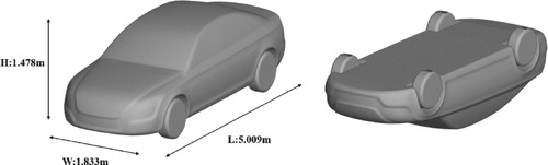
A simplified full-size model of an actual sedan was introduced. The overtaken sedan (Car 1) is the same as the overtaking sedan (Car 2). The shape and main geometrical parameters of the sedan model are shown in Figure 3. The frontal projection area of the car is 2.334 m². At a velocity of 20 m/s, the Reynolds number of the sedan is 6.846$\times$10⁶. Some accessories, such as the side-view mirrors, wipers and door handles were ignored to improve the computational efficiency.

Figure 3. Simplified car model.

2.4. Computational setup for aerodynamics

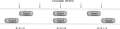
The computational domain for the aerodynamic forces computation is shown in Figure 4. Car 1 and Car 2 move forward at velocities of 20 and 30 m/s, respectively. The crosswind is perpendicular to the inlet wall and the velocity is constant at 10 m/s. As shown in Figure 5, a proportionality factor X / L was introduced to describe the relative position of the sedans in the longitudinal direction conveniently, where X is the distance between the rear and front sedans, and L is the length of the sedan. The initial relative position, X / L was set to −6, and the lateral spacing between the two sedans was set to 1 m.

Figure 4. Computational domain.

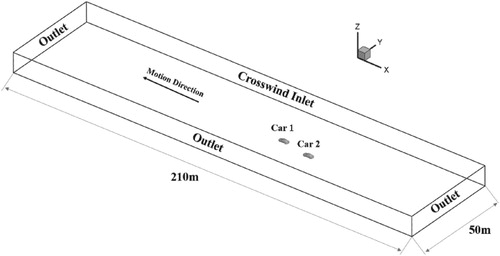
Figure 5. X / L in overtaking maneuver.

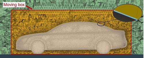
With consideration for good adaptability, the tetrahedral grid was applied to the entire computational domain (Figure 6). A moving box wrapping the car was created to avoid computational divergence due to the mesh distortion around the car, and the motion of the moving box is synchronous with the car.

Figure 6. Part of the computational mesh.

The mesh independence was performed by the comparison of the aerodynamic drag at different mesh schemes. Five different grid schemes were formed by adjusting the grid size of the moving box and the body surface. The overtaking car and the overtaken car move along a straight line without coupling. The aerodynamic forces of the overtaken car at X / L = −3 is the criteria, as shown in Table 1. The results show that when the number of elements is more than 11 million, the changes in the aerodynamic drag is very small. Considering the computational resources, the scheme 3 is chosen. The vehicle surface resolution ranged from 2 to 10 mm after adjusting the grid around the A-pillar, fenders and wheels. In order to make the simulation results more accurate, the mesh topology is divided into several regions in spatial resolution. The finest region is the boundary layers, there are 6 prism layers generated near the surface of sedan to capture the boundary layer and obtain the wall y+ around 30. The thickness of the first layer is 1 × 10⁻⁵ m and the growth rate is 1.2. The second region is the moving box, which captures details of the structure of the flow around the sedan. The third region is outside the moving box and simulates the flow in the entire computing domain.

Table 1. Aerodynamic forces of car 1 in different mesh strategies.

	Scheme 1	Scheme 2	Scheme 3	Scheme 4	Scheme 5
Number of elements	6168964	8685879	11188356	14571645	17876983
Drag (N)	229.6	224.3	220.4	219.3	219.0
Lateral force (N)	−360.9	−353.5	−349.2	−348.4	−348.0

The SIMPLE algorithm was selected for the iterative solution of the RANS equations. A hybrid second-order upwind/bounded central-differencing scheme for spatial discretization and a second-order scheme for temporal discretization were used (Mou et al., 2017).

The grid will be continuously updated with the movement of the car model, and the time step will determine the scale of the grid update. Therefore, a suitable time step must be selected to ensure the quality of the updated grid. In similar studies, the time step of the simulation is usually between 0.0002s and 0.005s (Clarke & Filippone, 2007; Liu et al., 2018; Salati et al., 2018). The grid is updated at each time step, thus a smaller time step will greatly increase the computation time, and the grid will have a large displacement in a long time step, which will increase the difficulty of re-meshing or even cause the failure of re-meshing. By considering the difficulty of re-meshing and the computation time, the time step was finally set to 0.001s.

2.5. Computational setup for multi-body dynamics

To obtain the dynamic response, a multi-body dynamics model was constructed according to the structure and performance parameters. As shown in Figure 7, the dynamic model was divided into ten subsystems, including rigid body, front and rear suspension, power, steering, and tire. The front suspensions are MacPherson suspensions, whereas the rear are multi-link suspensions. The magic formula tire model was introduced to obtain the accurate forces and moments of the tires (Pacejka & Bakker, 1992). Finally, the dynamic model which has 68 moving components, 62 constraints, and 160 degrees of freedom was constructed. In this study, a 2d_flat road with friction factor of 0.7 was used. The detailed parameters about the sedan are listed in Table 2.

Figure 7. MBD model.

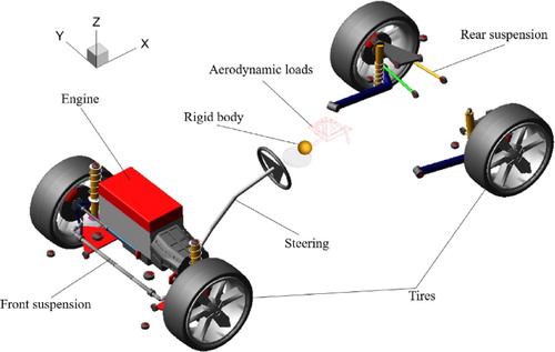
Table 2. Main parameters of the MBD model.

Parameter	Value	Units
Mass	1792	kg
Distance from the CM to the front wheel	1.227	m
Distance from the CM to the rear wheel	1.593	m
Height of CM	0.538	m
Wheel track	1.552	m
Moment of inertia about X axis	901	kg·m^2
Moment of inertia about Y axis	5910	kg·m^2
Moment of inertia about Z axis	5584	kg·m^2

3. Model validation

3.1. Verification of numerical model

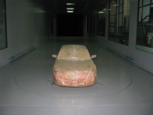
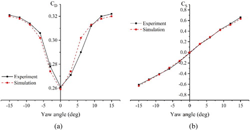
A 1:3 scale model wind tunnel test is performed in the HD-2 wind tunnel of Hunan University to verify the turbulence model and discretization scheme selection in the aerodynamic calculation (Figure 8). In the wind tunnel, the velocity of the airflow is 30 m/s. The aerodynamic drag and lateral force at different yaw angles are measured. The yaw angle varies from −15° to 15°, and the data are collected every 3°.

Figure 8. Scale model in wind tunnel test.

Meanwhile, the corresponding numerical simulation were performed. The results comparison with the wind tunnel test plotted in Figure 9 revealed that the aerodynamic drag coefficient and aerodynamic lateral force coefficient obtained by numerical computation are in good agreement with the experimental results.

Figure 9. The comparisons between experiment and computational results: (a) The drag force coefficient, (b) The lateral force coefficient.

3.2. Robustness of multi-body dynamics model

The motion of the car changes constantly during the overtaking process in crosswinds. Thus, the dynamic model should be robust. The input parameters to the dynamic model is uncertain due to the real-time aerodynamic forces. Hence, a parameter study, where the step forces with different magnitudes and directions were imposed at the reference point of the body, was performed to demonstrate the robustness of the dynamics model. Then, the dynamic response was obtained with the sedan driving at a constant velocity and fixed steering wheel (Figure 10). Finally, the robustness was confirmed by comparing the output of the MBD model with the theoretical expectation.

Figure 10. Response of the MBD model under different inputs: (a) Yaw angle, (b) roll angle, and (c) – (d) pitch angle.

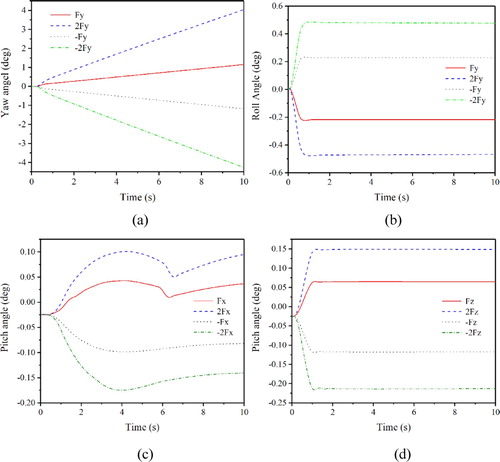
Figure 10(a) shows that the yaw angle changes with different side forces (Fy) imposed at the reference point. As the force doubled, the yaw angle not only increased accordingly, but also continuously increased due to the insufficient lateral adhesion. In addition, the roll angle of the car body plotted in Figure 10(b) showed that the roll angle increases as the side force increases. When the direction of the force changed, the direction of the yaw angle and the roll angle will also change accordingly.

Theoretically, because the reference point was located at the longitudinal symmetry plane of the car, the longitudinal force (Fx) and vertical force (Fz) affect the pitch angle of the car. The positive Fx or Fz imposed at the reference point induces positive pitch angle because the reference point is located at the northwest of the pitch center (Figures 10(c) and (d)). As the forces increase, the pitch angle also has the same changes as the theoretical expectation. The magnitude and trend of the positive and negative pitch angles are different when the direction of the forces changes because the stiffness of the front and rear suspensions is different. Therefore, the results of the parameter study show that the proposed dynamic model has good robustness and can accurately capture the dynamic response.

4. Results and analyses

4.1. Aerodynamic performance

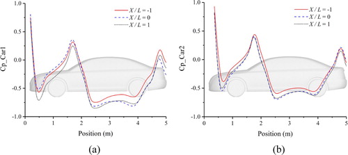
The variation of aerodynamic forces during overtaking maneuver plotted in Figure 11 showed that, in the overtaking maneuver, the aerodynamic drag of Car 1 starts to increase from X / L = −1 and peaks at approximately X / L = 0. The change of the aerodynamic drag can be explained by the pressure coefficient distribution on the body surface plotted in Figure 12. When Car 2 is parallel to Car 1, the pressure in front of Car 1 is the maximum while the rear is the minimum. The change in the pressure difference between the front and rear of the body can account for the variation in aerodynamic drag. The lateral force reaches the minimum at approximately X / L = −0.6. The pressure on the leeward side of Car 1 gradually increases as Car 2 approaches, thereby resulting in a decrease in lateral force. Moreover, the position, where the minimum lateral force occurs, is related to the velocity of the car and the crosswind. The magnitude of the yaw moment is related to the position of the reference point, but the variation is consistent with the lateral force.

Figure 11. Aerodynamic forces in overtaking: (a) Aerodynamic drag, (b) Lateral force, (c) Yaw moment.

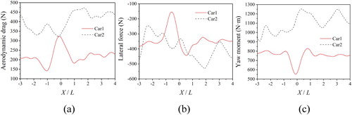
Figure 12. Pressure coefficient along longitudinal symmetry plane: (a) Car 1, (b) Car 2.

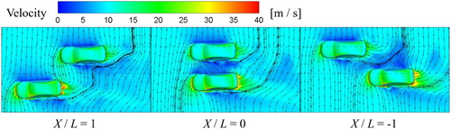
The flow fields at different positions during overtaking are shown in Figure 13. Contrary to Car 1, Car 2 is always in the unstable flow field induced by Car 1(Premoli et al., 2016). Thus, the variation of the aerodynamic forces and moments of Car 2 is relatively complex. In summary, the aerodynamic drag of Car 2 is much greater than that of Car 1 due to the faster velocity Car 2. As the pressure difference between the front and rear of the car decreases, the drag of Car 2 reaches the minimum at approximately X / L = 0. When Car 2 exceeds Car 1, the aerodynamic drag of Car 1 considerably increases due to the reduction of the influence of the flow field of Car 1. The results also show that the yaw moment of Car 2 generally increases, which can be interpreted by the movement of the pressure center induced by the increase in the yaw angle.

Figure 13. Snapshots of velocity distributions.

4.2. Dynamic response

The snapshots of velocity distributions at different moments plotted in Figure 13 showed that, due to the crosswind and flow field interaction between two cars, the lateral displacement and yawing motion are induced during overtaking. The posture of the car body is changed substantially as the overtaking maneuver progressed. The increase in the lateral space of the two cars weakens the interaction between the flow fields around the two cars, thereby resulting in a smaller variation of aerodynamic forces.

The vehicle displacements, such as the lateral displacement and yaw angle, are plotted in Figure 14. Generally, the yawing motion changes the posture of the car and the pressure center and further influences the aerodynamic performance. The lateral displacement affects the lateral space between two cars and the flow field around cars. When Car 2 gradually approaches to Car 1, the lateral force of the rear section of the car 1 decreases by the high-pressure area in the front end of Car 2. Thus, the lateral force difference between the front and rear sections of Car 1 is further increased. As a result, the yaw and lateral velocity of Car 1 are correspondingly increased compared with the single cars in crosswind. Otherwise, when Car 1 is overtaken by Car 2, the lateral force at the front of car 1 is reduced due to the external flow field at the rear of Car 2, thereby reducing the difference of the lateral force between the front and rear sections.

Figure 14. Dynamic response of Car 1 and Car 2: (a) Yaw angle, (b) Lateral displacement.

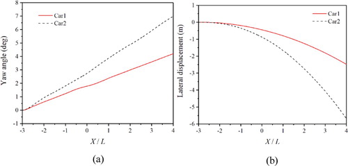
Moreover, the results show that the dynamic response of Car 2 is more intense than that of Car 1 due to its faster velocity. Hence, considering the influence of dynamic response is necessary when studying the aerodynamic performance of high-velocity vehicles.

4.3. Verification of the necessity of two-way coupling in overtaking

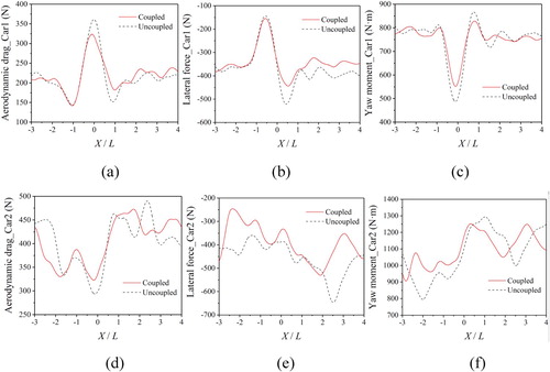
The aerodynamic forces obtained by the coupling method are compared with the results obtained by the uncoupling method to evaluate the effect of the two-way coupling on the simulation results (Figure 15). Notably, the aerodynamic forces obtained by the two methods are substantially different. In the case of coupling simulation, the fluctuations in aerodynamic drag, lateral force, and yaw moment of Car 1 are smaller than those in the uncoupling simulation. This discrepancy could be explained by the change in the aerodynamic performance induced by the feedback of the dynamic response. The aerodynamic forces acting on Car 2 are also substantially different from that of the uncoupled simulation, in the amplitude and phase. The result proved that the interaction between aerodynamics and vehicle dynamic response has a certain significance in ensuring the reliability of predicting the aerodynamic performance in overtaking under crosswind.

Figure 15. Aerodynamic forces in different method: (a)-(c) Aerodynamic drag, Lateral force, Yaw moment of Car 1; (d)-(f) Aerodynamic drag, Lateral force, Yaw moment of Car 2.

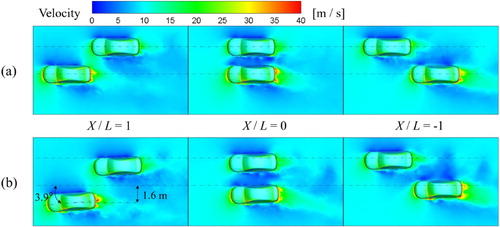
To further confirm the necessity of two-way coupling, several snapshots of velocity distribution at different moments are extracted (Figure 16). The posture and relative position of the two cars are considerably changed in the two-way coupling simulation. The interaction between the two cars is weakened, given that the increase in lateral spacing of the two cars is induced by crosswinds. However, in other situations, such as in an opposite crosswind, the lateral spacing of the two cars gradually decreases during the overtaking maneuver, and the interaction becomes increasingly intense, thereby resulting in serious accident.

Figure 16. Snapshots of velocity distributions: (a) uncoupled, (b) two-way coupled.

5. Conclusions

A multi-cars two-way coupling method is proposed to investigate the aerodynamic performance and dynamic response of two cars during overtaking maneuver under crosswind. The dynamic mesh technology was used to realize the movement of the vehicles. In each time step, the aerodynamic forces in the CFD model and the dynamic responses in the MBD model were exchanged in real time. The corresponding results were compared with the results obtained by the uncoupling method to investigate the necessity of the two-way coupling and the absolute velocity setup in overtaking maneuver under crosswind.

The results showed that the aerodynamic drag of the overtaken car increases and the lateral force decreases when the overtaking car gradually approaches the overtaken car during overtaking. However, the aerodynamic forces of the overtaking car are relatively complex because it is located at the unstable wake of the overtaken car. The yaw angle and lateral displacement of the overtaking car are much larger than the overtaken car. Moreover, the aerodynamic and dynamic response are considerably influenced by the changes of the posture and relative position of the overtaking and overtaken car. Therefore, using a multi-car two-way coupling method is necessary to avoid an unrealistic result when these responses are ignored.

The current research also revealed that the crosswinds cause the two cars to become distant from each other, thereby weakening the influence of the overtaking maneuver. Actually, when the direction of the crosswind or the relative position of the two cars changes, the overtaking maneuver greatly affects the aerodynamic performance and dynamic response of the two cars. Moreover, in real driving environment, the driver will respond to any external disturbance. Adding the driver model in the simulation is more realistic. Therefore, the influence of the crosswind direction and the driver response should be further revealed in future work.

Acknowledgements

The research was supported by the National Natural Science Foundation of China (grant number 51775395), State's Key Project of Research and Development Plan (grant number 2018YFB0105301) and the Fundamental Research Funds for the Central Universities (WUT: 2017II18XZ).

Disclosure statement

No potential conflict of interest was reported by the author(s).

Additional information

Funding

The research was supported by the National Natural Science Foundation of China [grant number 51775395], State's Key Project of Research and Development Plan [grant number 2018YFB0105301] and the Fundamental Research Funds for the Central Universities [WUT: 2017II18XZ].

References

- Akbarian, E., Najafi, B., Jafari, M., Ardabili, S. F., Shamshirband, S., & Chau, K. W. (2018). Experimental and computational fluid dynamics-based numerical simulation of using natural gas in a dual-fueled diesel engine. Engineering Applications of Computational Fluid Mechanics, https://doi.org/10.1080/19942060.2018.1472670
- Azim, A. F. A. (1994). An experimental study of the aerodynamic interference between road vehicles. SAE Technical Paper. https://doi.org/10.4271/940422
- Blocken, B., & Toparlar, Y. (2015). A following car influences cyclist drag: CFD simulations and wind tunnel measurements. Journal of Wind Engineering and Industrial Aerodynamics. https://doi.org/10.1016/j.jweia.2015.06.015
- Clarke, J., & Filippone, A. (2007). Unsteady computational analysis of vehicle passing. Journal of Fluids Engineering. https://doi.org/10.1115/1.2427085
- Du, T.-Z., Huang, C.-G., Wang, Y.-W., & Fang, X. (2010). Investigation of dynamic mesh technique and unsteady cavitation flows. Shuidonglixue Yanjiu Yu Jinzhan/Chinese Journal of Hydrodynamics Ser. A. https://doi.org/10.3969/j.issn.1000-4874.2010.02.008
- Fluent, a. (2009). ANSYS Fluent 12.0 user’s guide. https://doi.org/10.1016/0140-3664(87)90311-2
- Gu, Z. (2008). Numerical simulation analysis of external flow field of wagon-shaped car at the moment of passing. Chinese Journal of Mechanical Engineering (English Edition). https://doi.org/10.3901/cjme.2008.04.076
- Howell, J., Garry, K., & Holt, J. (2014). The aerodynamics of a small car overtaking a truck. SAE International Journal of Passenger Cars - Mechanical Systems. https://doi.org/10.4271/2014-01-0604
- Huang, T., Gu, Z., Feng, C., & Zeng, W. (2018). Transient aerodynamics simulations of a road vehicle in the crosswind condition coupled with the vehicle’s motion. Proceedings of the Institution of Mechanical Engineers, Part D: Journal of Automobile Engineering. https://doi.org/10.1177/0954407017704609
- Koutsourakis, N., Bartzis, J. G., & Markatos, N. C. (2012). Evaluation of Reynolds stress, k-ε and RNG k-ε turbulence models in street canyon flows using various experimental datasets. Environmental Fluid Mechanics. https://doi.org/10.1007/s10652-012-9240-9
- Lewington, N., Ohra-aho, L., Lange, O., & Rudnik, K. (2017). The Application of a one-way coupled aerodynamic and multi-body dynamics simulation process to predict vehicle response during a severe crosswind event. SAE Technical Paper Series. https://doi.org/10.4271/2017-01-1515
- Li, S., Gu, Z., Huang, T., Chen, Z., & Liu, J. (2018). Coupled analysis of vehicle stability in crosswind on low adhesion road. International Journal of Numerical Methods for Heat and Fluid Flow. https://doi.org/10.1108/HFF-01-2018-0013
- Liu, L. n., Wang, X. s., Du, G. s., Liu, Z. g., & Lei, L. (2018). Transient aerodynamic characteristics of vans during the accelerated overtaking process. Journal of Hydrodynamics. https://doi.org/10.1007/s42241-018-0029-2
- Margot, X., Hoyas, S., Fajardo, P., & Patouna, S. (2010). A moving mesh generation strategy for solving an injector internal flow problem. Mathematical and Computer Modelling, https://doi.org/10.1016/j.mcm.2010.03.018
- Mou, B., He, B. J., Zhao, D. X., & Chau, K. W. (2017). Numerical simulation of the effects of building dimensional variation on wind pressure distribution. Engineering Applications of Computational Fluid Mechanics. https://doi.org/10.1080/19942060.2017.1281845
- Nakasato, K., Tsubokura, M., Ikeda, J., Onishi, K., Ota, S., Takase, H., Akasaka, K., Ihara, H., Oshima, M., & Araki, T. (2017). Coupled 6DoF motion and aerodynamic crosswind simulation incorporating driver model. SAE International Journal of Passenger Cars - Mechanical Systems. https://doi.org/10.4271/2017-01-1525
- Nakashima, T., Tsubokura, M., Ikenaga, T., & Doi, Y. (2010). HPC-LES for unsteady aerodynamics of a heavy duty truck in wind gust - 2nd report: Coupled Analysis with Vehicle Motion. https://doi.org/10.4271/2010-01-1021
- Nakashima, T., Tsubokura, M., Ikenaga, T., Kitoh, K., & Doi, Y. (2011). Coupled analysis of unsteady aerodynamics and vehicle motion of a heavy duty truck in wind gusts. https://doi.org/10.1115/fedsm-icnmm2010-30646
- Nakashima, T., Tsubokura, M., Vázquez, M., Owen, H., & Doi, Y. (2013). Coupled analysis of unsteady aerodynamics and vehicle motion of a road vehicle in windy conditions. Computers and Fluids. https://doi.org/10.1016/j.compfluid.2012.09.028
- Noger, C., & Grevenynghe, E. V. (2011). On the transient aerodynamic forces induced on heavy and light vehicles in overtaking processes. International Journal of Aerodynamics. https://doi.org/10.1504/ijad.2011.038851
- Okumura, K., & Kuriyama, T. (2010). Transient aerodynamic simulation in crosswind and passing an automobile. SAE Technical Paper Series. https://doi.org/10.4271/970404
- Ortiz, J., & Bir, G. (2012). Verification of new MSC.ADAMS linearization capability for wind turbine applications. https://doi.org/10.2514/6.2006-785
- Pacejka, H. B., & Bakker, E. (1992). The magic formula tyre model. Vehicle System Dynamics. https://doi.org/10.1080/00423119208969994
- Premoli, A., Rocchi, D., Schito, P., & Tomasini, G. (2016). Comparison between steady and moving railway vehicles subjected to crosswind by CFD analysis. Journal of Wind Engineering and Industrial Aerodynamics. https://doi.org/10.1016/j.jweia.2016.07.006
- Salati, L., Schito, P., Rocchi, D., & Sabbioni, E. (2018). Aerodynamic study on a heavy truck passing by a Bridge Pylon under crosswinds using CFD. Journal of Bridge Engineering, https://doi.org/10.1061/(ASCE)BE.1943-5592.0001277
- Salih, S. Q., Aldlemy, M. S., Rasani, M. R., Ariffin, A. K., Ya, T. M. Y. S. T., Al-Ansari, N., Yaseen, Z. M., & Chau, K. W. (2019). Thin and sharp edges bodies-fluid interaction simulation using cut-cell immersed boundary method. Engineering Applications of Computational Fluid Mechanics. https://doi.org/10.1080/19942060.2019.1652209
- Sun, H., Karadimitriou, E., Li, X. M., & Mathioulakis, D. (2019). Aerodynamic Interference between Two road vehicle models during overtaking. Journal of Energy Engineering. https://doi.org/10.1061/(asce)ey.1943-7897.0000601
- Telionis, D. P., Fahrner, C. J., & Jones, G. S. (1984). An experimental study of highway aerodynamic interferences. Journal of Wind Engineering and Industrial Aerodynamics. https://doi.org/10.1016/0167-6105(84)90021-7
- Uystepruyst, D., & Krajnović, S. (2013). Numerical simulation of the transient aerodynamic phenomena induced by passing manoeuvres. Journal of Wind Engineering and Industrial Aerodynamics. https://doi.org/10.1016/j.jweia.2012.12.018
- Wang, J. Y., & Hu, X. J. (2012). Application of RNG k-ε turbulence model on numerical simulation in vehicle external flow field. Applied Mechanics and Materials. https://doi.org/10.4028/www.scientific.net/amm.170-173.3324
- Wang, Y., Zhang, Z., Zhang, Q., Hu, Z., & Su, C. (2020). Dynamic Coupling Analysis of Aerodynamic Performance of a Sedan Passing through a Bridge Pylon in Crosswind. Applied Mathematical Modelling. https://doi.org/10.1016/j.apm.2020.07.003
- Warsi, Z. U. A. (1981). Conservation form of the navier-stokes equations in general nonsteady coordinates. AIAA Journal. https://doi.org/10.2514/3.7763
- Winkler, N., Drugge, L., Trigell, A. S., & Efraimsson, G. (2016). Coupling aerodynamics to vehicle dynamics in transient crosswinds including a driver model. Computers and Fluids. https://doi.org/10.1016/j.compfluid.2016.08.006
- Yakhot, V., & Orszag, S. A. (1986). Renormalization group analysis of turbulence. I. Basic theory. Journal of Scientific Computing. https://doi.org/10.1007/BF01061452
- Yamamoto, S., Yanagimoto, K., Fukuda, H., China, H., & Nakagawa, K. (1997). Aerodynamic influence of a passing vehicle on the stability of the other vehicles. JSAE Review. https://doi.org/10.1016/S0389-4304(96)00063-X
- Zhang, Q, Su, C, & Wang, Y. (In press). Numerical Investigation on Aerodynamic Performance and Stability of a Sedan under Wind-Bridge-Tunnel Road Condition. Alexandria Engineering Journal. https://doi.org/10.1016/j.aej.2020.07.004
- Zhang, Q., Su, C., Zhou, Y., Zhang, C., Ding, J., & Wang, Y. (2020). Numerical Investigation on Handling Stability of a Heavy Tractor Semi-trailer under Crosswind. Applied Sciences. https://doi.org/10.3390/app10113672