Potential of kernel and tree-based machine-learning models for estimating missing data of rainfall

Abstract

In this study, two kernel-based models were used which include Support Vector Regression (SVR) and Gaussian Process Regression (GPR) and were compared with two tree-based models that are M5 and Random Forest (RF) for estimating missing monthly precipitation data in Antakya, Dortyol, Iskenderun and Samandag stations, which are the important precipitation stations in the Eastern Mediterranean region, Turkey. For this purpose, firstly 10% random precipitation data were assumed as missing data for the period 1980-2019. Secondly, the missing data in each station was estimated with the data of other stations within the framework of four data combinations scenarios. In Kernel-based SVR and GPR methods, the RBF kernel gave suitable results for the selected study area. While SVR and RF methods gave very close estimation results, the SVR method gave relatively better results than the other methods especially in error minimizing aspects. Gaussian function based GPR model generally tries to estimate missing data closer to means. This is the main disadvantage of the GPR model and therefore it is unsuccessful in the estimation process. Finally, the results showed that the algorithms based on machine learning are successful in estimating the missing precipitation data.

KEYWORDS:

• Missing data
• rainfall
• machine learning
• random Forest
• Eastern Mediterranean
• Turkey

Introduction

With the increase in the population recently, it is seen that the rains show a more irregular pattern as a result of climate change. In this case, meeting the nutritional needs of the increasing population may be possible with an effective agricultural irrigation management activity depending on precipitation.

Rainfall is one of the most important inputs of hydrological systems and plays a key role in all water management studies. Accurate measurement of precipitation is very important in flood prediction and control, drought analysis, flow modeling, sediment control and management, basin management, agricultural irrigation planning, and water quality studies. Accurate detection of precipitation in cities and rural areas is also important for the prevention and management of flood disasters.

The amount of precipitation is measured at certain period intervals at precipitation observation (or synoptic) stations like other climate variables. However, measurement errors based on human or device reasons, or the fact that precipitation is not measured for any reason at any given time, may disrupt the water managers’ plans. Robust precipitation data are indispensable for all kinds of forecasts and calculations in hydrology and meteorology studies. Missing data can lead to incorrect planning. Estimating the missing data in the precipitation time series is the first stage of each scientific study.

In the past studies, missing data was generally replaced by simple statistical methods such as arithmetic average. However, with the help of models such as artificial intelligence and machine learning based on data, more accurate estimations can be made with rainfall data measured in the same region and at the same period in neighboring stations with the same climate conditions, regardless of the physics of the precipitation event (Sattari et al., 2018).

In neighboring and similar meteorological stations, the precipitation measured in the same period can be defined as the input of the machine learning models and the measured precipitation data of the target station as output, and the model can be trained. Then, with the help of models that pass the test process successfully, the missing precipitation values in the target station can be estimated.

Today, with the increase of data banks and the advancement of computer technology, the use of data-based models has increased in all scientific fields in predictive aims. In the case that there is a significant statistical connection and correlation between the input and output data of each system, the data entering and leaving the system can be trained to the machine and future predictions can be made without considering the physics of the event.

Machine learning algorithms applied in almost all fields of hydrology and meteorology sciences. ML utilized in modeling the amount of pan evaporation (Shabani et al., 2020), reservoir operation (Rouzegari et al., 2019), the modeling of groundwater levels (Sattari et al. 2018), on the forecasting maximum precipitation for long terms (Nourani et al., 2017), surface water quality parameters estimation (Sattari et al., 2016), classification of groundwater quality (Saghebian et al., 2014), daily river flows (Apaydin et al., 2020, Sattari et al., 2012, 2013) have been studied.

Nkuna and Odiyo (2011) completed the missing rainfall data based on the measured values in the precipitation observation station in the Luvuvhu river basin in South Africa by using the Radial based ANN method. More recently, Rajab Homsi et al. (2020) utilized a multi-criteria decision analysis and symmetrical uncertainty to recognize the suitable general circulation models for precipitation projections. Another survey paper proposed by Fotovatikhah et al. (2018) applied computational intelligence in terms of single and hybrid methods for the flood management system to identify the best ensemble ML methods for flood debris forecasting and management. Shamshirband et al. (2020) applied three machine learning methods such as SVM, GEP, and MT for the prediction of Standardized Precipitation Index (SPI), Standardized Streamflow Index (SSI), and Standardized Precipitation Evapotranspiration Index (SPEI). Ghorbani et al. (2018) made use of a quantum behaved PSO which embedded in MLP to forecast the evaporation rates over a daily forecast horizon. Qasem et al. (2019) investigated the efficiency of combined SVR with wavelet for predicting evaporation rates at Tabriz (Iran) and Antalya (Turkey) stations. Moazenzadeh et al. (2018) used a firefly algorithm integrated with support vector regression (SVR) to predict evaporation in northern Iran. A study by Che Ghani et al. (2014) successfully estimated the missing data in precipitation datasets with the genetic programming method in Malaysia. A research conducted by Bakiş and Göncü (2015), estimated the inflow missing data in the Zap basin, in Turkey by using linear and nonlinear multivariate regression methods based on the correlation values between hydrometric stations.

Githungo et al. (2016) successfully found 153 missing precipitation data from 9 precipitation observation stations in arid and semi-arid climates of Kenya by using satellite data.

A study carried out by Sattari et al. (2018) estimated monthly precipitation data by using data mining and traditional statistical methods at 6 precipitation observation stations in East Azerbaijan province, northwest of Iran. The decision tree method showed successful performance according to the results of their study.

Bielenki Junior et al. (2018) determined the missing monthly precipitation data in Brazil's Rio das Cinzas basin using GIS-based techniques. They successfully filled the gaps in the Python software environment by coding based on Thiessen polygons and inverse distance weights (IDW) approaches.

Research by Nelsen et al. (2018) found the missing temperature data in Utah, the USA for a period of 3 months to 5 years, based on the empirical Mode Decomposition (EMD) approach. They developed the estimation model based on the correlations between the stations and the periodic behavior of data in each station.

Kamwaga et al. (2018) completed the missing data in 19-year time-series flow data by using experimental, univariate, and multivariate regression methods in a basin in Tanzania. In Tanzania basins, missing data is a common problem inflow data sets. In these conditions, the use of regression methods for completing missing flow data emphasized by researchers.

A study by Vega-Garcia et al. (2019) tried to estimate the missing daily flow data in Spain by using the cascade-correlation ANN method for filling the gaps. According to their results, the model is more successful for short periods before and after the gap. The model showed that the correlation coefficient ranged from 0.75 to 0.80 in low-water-flow periods.

Canchala-Nastar et al. (2019) completed the missing data in the flow data of 1983–2016 in 45 hydrometric stations in the southwest of Colombia with Principal Component Analysis based ANN method. In the study, it was seen that the nonlinear Principal Component Analysis based ANN method gave successful results.

Dembélé et al. (2019) found daily missing flow data in the Volta river basin in West Africa with Direct Sampling (DS) used as a non-parametric stochastic method. They emphasized that the developed method can be used in similar areas and conditions.

Ozen and Bal (2020) estimated missing flow data via Random Forest (RF) and K-Nearest Neighborhood (KNN) methods in their study. They first produced artificial data with the Monte Carlo simulation and then estimated the missing data by using the RF method under various scenarios and compared the results with the results of the KNN method. The results showed that the KNN method could make a more accurate prediction for the structures with medium and low correlations.

Different studies applied kernel-based SVR-GPR and RF techniques to hydrology research, but these techniques were applied for few types of research to predict the missing precipitation data. This study aims to evaluate the performance of two groups of machine learning (kernel-based SVR and GPR, tree-based M5, and RF) methods for the estimation of monthly rainfall data in Antakya, Dortyol, Samandag and Iskenderun precipitation stations in the eastern Mediterranean region, Turkey.

Material and methods

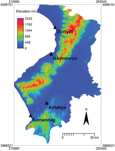
This study was conducted in Turkey's eastern Mediterranean region (Figure 1). In this region, summers are hot and dry, winters are warm and rainy. It has snowfall only a few days in a year. The temperature ranges from −6°C to + 43°C. At the higher points of the mountains, the temperature is lower than in the lowlands (URL1).

Figure 1. The map of study area.

In this study, monthly rains between January 1980 and December 2019 belonging to Antakya, Dortyol, Iskenderun, and Samandag precipitation stations were considered. The geographical locations of these stations and the statistical properties of the precipitation are given in Table 1.

Table 1. Statistics of precipitation data and geographic position of selected rain gauge stations.

	Antakya	Dortyol	Iskenderun	Samandag
Minimum (mm)	0	0	0	0
Maximum (mm)	298	285.3	283	433.6
Mean (mm)	90.18	80.1	62.9	75.01
Standard deviation (mm)	94.78	61.7	52.4	76.72
Aridity index	29.81	33.16	25.08	32.14
Elevation (m)	100	28	4	40
Latitude (Y)	36˚ 12’ 32'’ N	36˚ 51’ 31'’ N	36˚ 35’ 05'’ N	36˚ 05’ 29'’ N
Longitude (X)	36˚ 09’ 09'’ E	36˚ 11’ 53'’ E	36˚ 10’ 03'’ E	35˚ 59’ 26'’ E

The climate at each station was determined using the De Martonne (1923) aridity index (I) shown in Equation (1). (1) $\begin{array}{r}I=\frac{P}{T+10}\end{array}$(1) where P and T are the annual average precipitation (mm) and temperature (The conclusion section improved based on the reviwers comments.), respectively. According to the aridity index values (25–33) given in Table 1, the study area shows similarity in terms of climate. As can be seen from Table 1, very high precipitation occurred in some periods at all 4 stations and therefore standard deviations are seen to be high. Since these high rainfall values occur rarely, therefore machine-learning models are thought to be troublesome in learning these high and rare precipitation data.

Correlations between stations were considered in defining input and output variables in machine learning models. In this study, different combinations of inputs were considered in various scenarios. In Figure 2, the correlation matrix of the precipitation data at 4 stations is given visually.

Figure 2. Visual correlation matrix in precipitation data for study area stations.

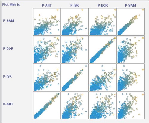
Figure 2 shows significant correlation between precipitation data in visualized format. All stations under study are located in the same climatic condition and are close and adjacent to each other. Also as can be seen in Figure 2, the data of Dortyol and İskenderun stations have been compared relatively compared to the other two stations. On the other hand the, points on the diagonal line shows that the precipitation of each station is in a 100% correlation with its precipitation values.

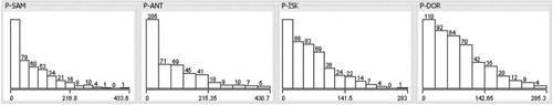
Histograms of precipitation data for all stations are given in Figure 3. It is represented in Figure 3 that naturally low precipitation cases are dominant and the number of extreme precipitation is very low.

Figure 3. The histogram of rainfalls in all stations.

Besides, to analyze the data, the linear projection graph for all stations is given in Figure 4 which is prepared through a linear projection method with explorative data analysis. As can be seen from Figure 4, except for some extreme rain values that appear naturally, other precipitation data fit into a cluster for each of the stations, so there are no outlier values.

Figure 4. Linear projection graph for selected stations rainfalls.

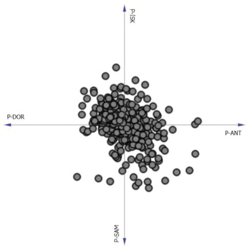
In this study, all four stations are located in the same region and under the same climatic conditions. Therefore, precipitation of all four stations shows a similar pattern. If outlier data is found at any station, the Linear projection graph can also show itself. In this study, it has been proven that there is no such situation, as a result of statistical tests in the XLSTAT environment. If the referee insists, these test results can be added to the study.

In this study, four different machine-learning techniques were utilized. Each technique is briefly discussed below.

Gaussian process regression (GPR)

Gaussian process regression is a full Bayesian learning algorithm which applied widely in practical application in terms of model training, hyperparameter estimation, and uncertainty estimation. Generally, in regression models, observed/measured values (x_i) and predicted values (y_i) are expected to be close to each other. This similarity expected in Gauss processes is presented by the covariance function. In the GPR models, the covariance function between two latent variables (x_i) and f(x_j) is determined for i≠j. In GPR models, the values of the noise are independent with mean zero and σ² variance, and the Gaussian explained with f(.) as a latent (unknown) function. The latent function that must be determined in the GPR model is f. In GPR studies after the data set is trained, the measured/observed input data turns into output with the help of f function (Rasmussen & Williams, 2005).

It was applied in the Missouri River for the modeling of daily water temperature from air temperature (Zhu et al., 2018).

Support vector regression (SVR)

Support Vector Machines are machine-learning algorithms developed by Vapnik and other researchers (Vapnik et al., 1997). This approach was originally developed as a way of interpreting sensor data and includes a two-layer structure. The first layer is a weightless nonlinear core on support vectors containing the input variable series, and the second is a weighted sum of core outputs. They are machine learning approaches in data-oriented research fields and are based on statistical learning theory. SVM is used to best distinguish two data classes. For this purpose, decision boundaries or hyperplanes are determined. Models of the SVM are divided into two main sections (a) the classifier models of the SVM and (b) the SVR model. An SVM model is used to solve the classification of data in various classes, and the SVR model is used for prediction purpose. Regression is used to obtain a hyperplane suitable for the data utilized. The distance to any point in this hyperplane indicates the error of that point.

In this study, four different kernel functions (polynomial, radial-basis function, Pearson VII function (PUK) and normalized polynomial kernels) that are most frequently included in the literature were used (Demirci, 2019).

M5

M5 decision tree method, which is one of the machine learning methods and is an effective, non-parametric, intensive computational method that can be applied to classification and regression problems. A decision tree is a model that can predict the value of a dependent variable by using the values of the independent variable set. There are two types of decision trees: (1) classification trees are the most common and a symbolic class used to estimate the value of a nominal attribute. (2) Regression trees used to predict numerical values. If each leaf in the tree contains a linear regression model used to predict the target variable in that leaf, then it is called a model tree (Witten & Frank, 2005). Quinlan (1992) originally developed the M5 decision tree algorithm. The M5 algorithm creates a regression sequence by repeatedly dividing the sample space using tests on a single attribute that maximizes the variance in the target space. If the obtained tree model is translated into ‘If-Then' format and is written as rules, it is also called the M5 Rule model.

Random Forest (RF)

Random Forest is an ensemble learning method that combines the results of decision trees generated by selecting samples from the same data set by a bootstrap method and can be used for both classification and regression purposes. It is commonly used in areas such as ecology, genetics, bioinformatics where the high-dimensional data takes place and can perform supervised or unsupervised learning. RF uses m variables, where m is less than the number of all predictor variables p, while splitting the nodes to create different trees and overcome the overfitting problem. It can give a generalization error for all trees in the forest and provides not only an intuitive measure of variable importance but also a proximity matrix that gives the distances between the observations (Özen & Bal, 2019).

Evaluation metrics

In this study, some common statistical parameters used in the comparison and selection of machine learning models were used. Differences between the measured and predicted precipitation data were determined by the Mean Absolute Error (MAE) and Root Mean Square Error (RMSE). The agreement between the observed and predicted values was measured by the correlation coefficient (R). (2) $\begin{array}{rl}\text{MAE}& =\frac{1}{N}\sum _{i=1}^N|X_i-Y_i|\end{array}$(2) (3) $\begin{array}{rl}\text{RMSE}& =\sqrt{\frac{1}{N}\sum _{i=1}^N{\left(X_i-Y_i\right)}^2}\end{array}$(3) (4) $\begin{array}{rl}R& =\frac{N\sum X_i{Y}_i-\left(\sum X_i\right)\left(\sum Y_i\right)}{\sqrt{N(\sum {X_i}^2)-{(\sum X_i)}^2}\sqrt{N(\sum {Y_i}^2)-{\left(\sum Y_i\right)}^2}}\end{array}$(4) where X_i and Y_i are the observed and predicted values, and N is the number of observations. Also, Taylor diagrams were utilized to check the accuracy of the applied models. In this diagram, measured and some corresponding statistical parameters can be observed simultaneously. Moreover, different points in the polar graph are used to investigate the differences between the observed and predicted values in the Taylor diagrams (Taylor, 2001).

Results

Since the meteorological stations used in this study have similar climatic conditions, the estimations made are based on the principle of the neighborhood between meteorological stations, which is well known in hydrology. In this study, four different scenarios of the measured data in the other station were taken into account for the estimation of missed precipitation data in each station, and estimations were made according to all methods used for each precipitation station. The precipitation data of each station was taken randomly as 10% missing data and this missing data was estimated with the help of Weka software according to GPR, SVR, M5, and RF machine learning techniques. As in the literature analysis we have done, in all hydrological studies, generally, the accuracy rate of the models is tested with parameters such as R, RMSE, and MAE. In this study, we used the Taylor diagram to evaluate model results. The compatibility between historical measured and predicted meteorological data is evaluated by scatter plot and time series graphics. This study took into account all the above-mentioned criteria similar to previous studies. The calculations of the Antakya station are given in Table 2.

Table 2. The results of modeling for Antakya station.

	Scenario	Inputs			Output	R	MAE (mm)	RMSE (mm)
GPR	1	İskenderun	Dortyol	Samandag	Antakya	0.93	58.35	73.07
	2	İskenderun	Dortyol		Antakya	0.89	64.45	80.63
	3	Dortyol	Samandag		Antakya	0.91	64.22	80.38
	4	İskenderun	Samandag		Antakya	0.92	64.52	80.13
SVR	1	İskenderun	Dortyol	Samandag	Antakya	0.93	34.41	49.22
	2	İskenderun	Dortyol		Antakya	0.90	42.47	58.49
	3	Dortyol	Samandag		Antakya	0.92	38.39	55.34
	4	İskenderun	Samandag		Antakya	0.92	35.92	51.99
M5	1	İskenderun	Dortyol	Samandag	Antakya	0.92	29.16	43.40
	2	İskenderun	Dortyol		Antakya	0.89	36.40	50.11
	3	Dortyol	Samandag		Antakya	0.92	32.16	44.81
	4	İskenderun	Samandag		Antakya	0.92	29.25	43.30
RF	1	İskenderun	Dortyol	Samandag	Antakya	0.93	26.37	39.68
	2	İskenderun	Dortyol		Antakya	0.84	36.63	56.33
	3	Dortyol	Samandag		Antakya	0.94	27.20	38.56
	4	İskenderun	Samandag		Antakya	0.91	30.46	43.58

All kernel functions were examined during the SVR and RF modeling process. Based on the results, RBF kernel function was determined as the best for both SVR and RF models. Based on the Weka outputs, the optimum RBF kernel function parameters used in the simulation were as below (Gamma=0.01 and the cache size=250,007).

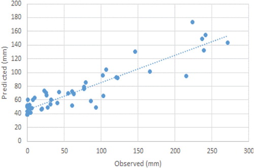
It can be seen from Table 2 that the estimation results are very close to each other in all models. According to GPR, SVR, and M5 methods, the first scenario gave the best results. According to this scenario, during the estimation of missing precipitation data in Antakya station, all rains in other stations were taken as model input, and higher accuracy was obtained. However, when it comes to the RF method, the third scenario gave the best result. In other words, according to the RF method, Dortyol and Samandag stations alone estimated the missing precipitation of Antakya station better than the other methods and scenarios with R = 0.94, MAE = 27.20 mm, and RMSE = 36.56 mm values. Thus, for the Antakya meteorological station, the RF method estimated missing precipitation data in the best way according to the third scenario (Figures 5 and 6).

Figure 5. Antakya station rainfall graph for observed and estimated missing data (RF scenario 3).

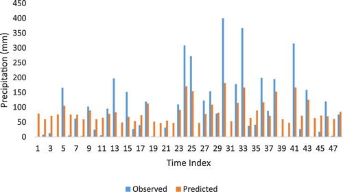
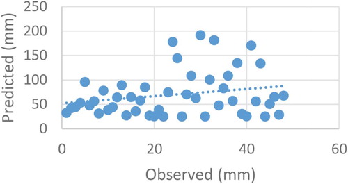
Figure 6. Scatter plot of missing and observed data at Antakya station (RF scenario 3).

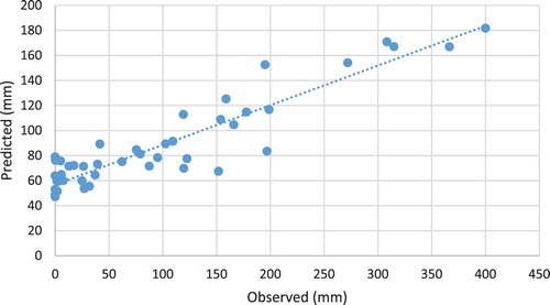
Figures 5 and 6 indicate the RF method excluding high and extreme values, which has successfully estimated the missing precipitation data at Antakya station. High and extreme values of the randomly selected 10% missing precipitation data for the model training at Antakya station naturally repeated in a small number (low frequency). In this case, the model suffered from learning and thus predicted high missed precipitation values as inaccurate and few.

To evaluate the performance of the models in detail in Antakya station, measured and the estimated missed precipitation values were compared (Table 3). The statistical values given in Table 1 cover all precipitation data sets, but the estimates made according to the models in Table 3 and also the values given in the last column for comparison purposes only belong to the 10% assumed as missing data. In Table 1, the standard deviation value of the Antakya station in all precipitation data set was 94.78 mm, but in Table 3, the standard deviation for the missing data, which randomly selected at Antakya station, was 105.98 mm and in a sense, it shows that there are more numbers of extreme precipitation values in the selected random precipitation data. This issue appears to affect the model results in a bad way.

Table 3. Comparison of observed and estimated monthly precipitation data in Antakya station.

	GPR	SVR	M5	RF
Statistic	Scenario 1	Scenario 1	Scenario 1	Scenario 3	Observed
Minimum (mm)	47.11	0.00	0.00	0.50	0.00
Maximum (mm)	181.70	259.12	288.64	311.73	400.10
Mean (mm)	85.38	72.73	82.53	79.79	90.06
Standard deviation (mm)	36.32	73.03	86.19	86.87	105.98
Correlation	0.93	0.93	0.92	0.94	1.00
Number of instances	48	48	48	48	48

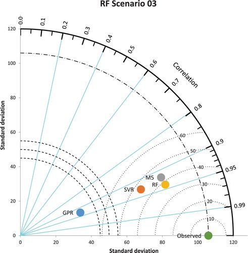
As can be seen from Table 3, the mean missed precipitation values estimated from the GPR (scenario 1) method are closer to the measured values, but when the other statistics analyzed, it is seen that the RF (scenario 3) method gives better results. The performance of the models for the Antakya station is given in the Taylor diagram for the visualization (Figure 7).

Figure 7. Taylor diagram for Antakya station.

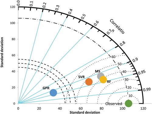
As can be seen from Figure 7, there is an important difference between the standard deviation value of the observed precipitation data and the standard deviation value of the estimated precipitation data in the GPR method in Antakya station. Due to the normal distribution nature of the GPR method, their estimates converge to average values. Due to this difference, the results obtained are not reliable.

In Table 4, the results of the estimated missed precipitation data of the Dortyol station are given based on the scenarios for each used model.

Table 4. The results of modeling for Dortyol station.

	Scenario	Inputs			Output	R	MAE (mm)	RMSE (mm)
GPR	1	Antakya	İskenderun	Samandag	Dortyol	0.87	40.81	47.63
	2	Antakya	İskenderun		Dortyol	0.86	43.40	50.34
	3	Antakya	Samandag		Dortyol	0.85	44.04	51.85
	4	İskenderun	Samandag		Dortyol	0.85	44.77	52.53
SVR	1	Antakya	İskenderun	Samandag	Dortyol	0.87	26.35	34.29
	2	Antakya	İskenderun		Dortyol	0.86	28.16	35.50
	3	Antakya	Samandag		Dortyol	0.85	30.06	38.26
	4	İskenderun	Samandag		Dortyol	0.85	29.03	37.37
M5	1	Antakya	İskenderun	Samandag	Dortyol	0.86	26.63	34.97
	2	Antakya	İskenderun		Dortyol	0.85	27.76	35.63
	3	Antakya	Samandag		Dortyol	0.85	29.37	36.73
	4	İskenderun	Samandag		Dortyol	0.85	26.58	35.48
RF	1	Antakya	İskenderun	Samandag	Dortyol	0.86	27.14	34.44
	2	Antakya	İskenderun		Dortyol	0.84	26.85	37.48
	3	Antakya	Samandag		Dortyol	0.76	34.28	43.36
	4	İskenderun	Samandag		Dortyol	0.82	28.97	38.64

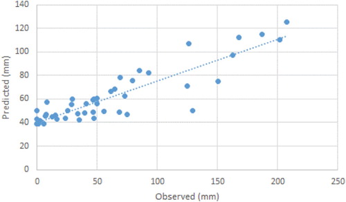
It can be seen from the results of the Dortyol station in Table 4, the first scenario in which all stations are considered as input, yielded relatively good results compared to other scenarios. Here, in the first scenario, the Dortyol station is output and the other three stations are input. Also, it is visible that the results of all four estimation models used at Dortyol station are very close to each other. According to the results, at this station the SVR method (R = 0.87, MAE = 26.35 mm and RMSE = 34.29 mm) gave the best results compared to other techniques. Comparison charts for this result are given in Figures 8 and 9.

Figure 8. Exchange graph of observed and estimated missing data of Dortyol station (SVR scenario 1).

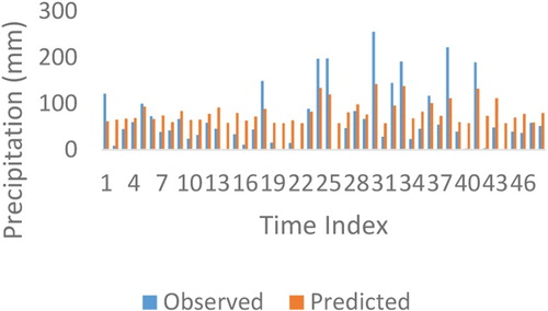
Figure 9. Scatter plot graph of observed and estimated lost data of Dortyol station (SVR scenario 1).

As can be seen from Figures 8 and 9, the SVR model could not estimate extreme values well. The main reason for this failure is the extreme and high precipitation values in the randomly selected data. The results of the four models are given in Table 5 with a comparison match in detail.

Table 5. Comparison of measured and estimated missed monthly precipitation data in Dortyol station.

	GPR	SVR	M5	RF
Statistic	Scenario 1	Scenario 1	Scenario 1	Scenario 1	Observed
Minimum (mm)	57.58	25.46	23.52	6.46	0.00
Maximum (mm)	142.51	191.82	214.07	226.04	255.80
Mean (mm)	80.02	70.00	77.27	77.70	68.55
Standard deviation (mm)	23.40	45.59	53.35	56.57	65.38
Correlation	0.87	0.87	0.86	0.86	1.00
Number of instances	48	48	48	48	48

It is understood from Table 5 that although the SVR technique gives the best result according to the mean and correlation coefficient at the Dortyol station, RF method gave the best performance in terms of minimum, maximum and standard deviation based on the first scenario results. In Figure 10, the performance of the used methods in Dortyol station is given visually via the Taylor diagram based on the first scenario results.

Figure 10. Taylor diagram for Dortyol station.

It is noticed from Figure 10 that when we considered all the statistical model selection criteria in the estimation of missed precipitation data at Dortyol station, the most reliable result was of RF and the worst result was of the GPR method.

The results of the models utilized for the İskenderun station are given in Table 6 for each of the four different scenarios.

Table 6. The results of modeling for İskenderun station.

	Scenario	Inputs			Output	R	MAE (mm)	RMSE (mm)
GPR	1	Antakya	Dortyol	Samandag	İskenderun	0.89	29.92	38.09
	2	Antakya	Dortyol		İskenderun	0.88	31.87	40.66
	3	Antakya	Samandag		İskenderun	0.89	34.20	42.49
	4	Dortyol	Samandag		İskenderun	0.87	33.84	43.42
SVR	1	Antakya	Dortyol	Samandag	İskenderun	0.89	18.69	27.01
	2	Antakya	Dortyol		İskenderun	0.88	19.53	27.76
	3	Antakya	Samandag		İskenderun	0.89	21.73	29.19
	4	Dortyol	Samandag		İskenderun	0.87	22.36	31.13
M5	1	Antakya	Dortyol	Samandag	İskenderun	0.89	19.07	25.99
	2	Antakya	Dortyol		İskenderun	0.88	19.63	26.83
	3	Antakya	Samandag		İskenderun	0.89	21.74	26.87
	4	Dortyol	Samandag		İskenderun	0.88	20.64	27.93
RF	1	Antakya	Dortyol	Samandag	İskenderun	0.86	20.64	29.22
	2	Antakya	Dortyol		İskenderun	0.87	21.02	28.05
	3	Antakya	Samandag		İskenderun	0.80	24.47	34.18
	4	Dortyol	Samandag		İskenderun	0.85	21.23	1.31

From Table 6 it can be seen that the first scenario in SVR model (R = 0.89, MAE = 18.69 mm and RMSE = 27.01 mm) gave the best result. As mentioned earlier in the SVR model, the RBF kernel performed better than the other kernels. The results of other techniques seem to be almost close to the SVR method. In Iskenderun station, the first scenario gave the best results compared to all other techniques and scenarios except the RF technique in the modeling of missed precipitation data. According to the first scenario, Iskenderun station is output and the other stations are taken as input. However, in the second scenario, only Antakya and Dortyol stations were considered as inputs. The first scenario results of the SVR model, which gives the best results for the Iskenderun station, are graphically given in Figures 11 and 12.

Figure 11. Change plot of observed and estimated missing data of İskenderun station (SVR scenario 1).

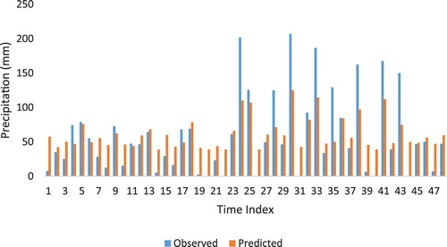
Figure 12. Scatter plot of observed and estimated missing data of İskenderun station (SVR scenario 1)

It can be understood from Figures 11 and 12 that the SVR method (first scenario) estimates the missed precipitation data of Iskenderun station at a relatively acceptable level.

Statistics for the estimation obtained from the models for the Iskenderun station were compared with the statistics of the measured values and the results are given in Table 7.

Table 7. Comparison of observed and estimated missed monthly precipitation data in Iskenderun station.

	GPR	SVR	M5	RF
Statistic	Scenario 1	Scenario 1	Scenario 1	Scenario 2	Observed
Minimum (mm)	38.73	7.05	9.12	2.57	0.00
Maximum (mm)	125.15	182.25	200.03	191.87	207.30
Mean (mm)	61.00	52.49	58.07	58.34	59.18
Standard deviation (mm)	22.63	45.90	49.22	49.71	57.24
Correlation	0.89	0.89	0.89	0.87	1.00
Number of instances	48	48	48	48	48

As can be seen from Table 7, the SVR model (Scenario 1) in terms of the correlation coefficient, M5 (Scenario 1) in terms of maximum value and RF (Scenario 2) model in terms of minimum, average and standard deviation gave the good results. The Taylor diagram of Iskenderun station is given in Figure 13.

Figure 13. The Taylor diagram of Iskenderun station.

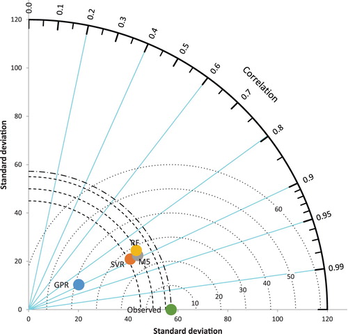
Figure 13 manifests that the GPR model at İskenderun station has been very unsuccessful in terms of standard deviation. However, other SVR, M5, and RF methods estimated similarly missing data in terms of standard deviation and other statistics. Samandag station was considered as the last station in the study. In Table 8, the estimation results of the missing data of this station are given according to different models and different scenarios.

Table 8. Samandag station missing data estimation results.

	Scenario	Inputs			Output	R	MAE (mm)	RMSE (mm)
GPR	1	Antakya	İskenderun	Dortyol	Samandag	0.92	40.00	48.94
	2	Antakya	İskenderun		Samandag	0.92	44.99	53.88
	3	Antakya	Dortyol		Samandag	0.91	43.84	53.42
	4	İskenderun	Dortyol		Samandag	0.87	47.28	58.43
SVR	1	Antakya	İskenderun	Dortyol	Samandag	0.92	22.10	31.02
	2	Antakya	İskenderun		Samandag	0.92	22.33	30.97
	3	Antakya	Dortyol		Samandag	0.91	22.41	32.67
	4	İskenderun	Dortyol		Samandag	0.88	29.15	41.64
M5	1	Antakya	İskenderun	Dortyol	Samandag	0.92	22.50	30.53
	2	Antakya	İskenderun		Samandag	0.92	24.33	30.98
	3	Antakya	Dortyol		Samandag	0.91	22.90	31.80
	4	İskenderun	Dortyol		Samandag	0.88	26.94	37.80
RF	1	Antakya	İskenderun	Dortyol	Samandag	0.93	20.38	28.19
	2	Antakya	İskenderun		Samandag	0.93	21.15	29.82
	3	Antakya	Dortyol		Samandag	0.91	22.20	32.09
	4	İskenderun	Dortyol		Samandag	0.85	29.89	40.58

As can be seen from Table 8, the first scenario was successful at Samandag station. In the first scenario, Samandag station output and the other 3 stations were model inputs. The RF (R = 0.93, MAE = 20.38 mm and RMSE = 28.19 mm) method gave very good results in estimating the missed precipitation at Samandag station. The results of the other machine learning methods appear to be almost close to the results of the RF method. The first scenario results of the RF model, which gave the best results for Samandag station, are graphically presented in Figures 14 and 15.

Figure 14. Change plot of observed and estimated missing data of Samandag station (RF scenario 1).

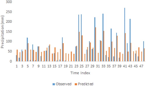
Figure 15. Scatter plot of observed and estimated missing data of Samandag station (RF scenario 1).

As can be seen from Figures 14 and 15, at the Samandag station, except for extreme values, other missing precipitation values were estimated following the observed values. Statistics of the values obtained from the models of Samandag station were compared with the observed values and the results are given in Table 9.

Table 9. Comparison of estimated and observed missing monthly precipitation data in Samandag station.

	GPR	SVR	M5	RF
Statistic	Scenario 1	Scenario 1	Scenario 1	Scenario 1	Observed
Minimum (mm)	38.74	0.00	0.73	0.51	0.00
Maximum (mm)	173.20	261.27	290.99	265.33	271.00
Mean (mm)	72.98	63.80	71.91	74.00	67.93
Standard deviation (mm)	33.71	66.49	73.58	73.02	78.13
Correlation	0.92	0.92	0.92	0.93	1.00
Number of instances	48	48	48	48	48

From Table 9 we can see that the SVR method in terms of minimum, RF in terms of maximum and correlation coefficient, M5 model in terms of mean and standard deviation gave the best result. Precipitation is completely random and stochastic, and it is naturally unexpected to achieve 100% accuracy. As can be seen in the literature review, the results obtained in this study are close to similar studies and acceptable levels. Taylor diagram of Samandag is given in Figure 16. The visualized performance of four methods used in this diagram in the estimation of missing data are graphically represented.

Figure 16. Taylor diagram for Samandag station.

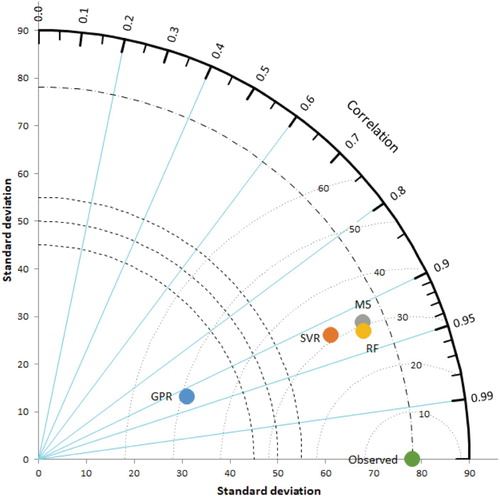
As can be seen from Figure 16, M5 and RF models results showed very similarity in Samandag station missing data precipitation estimations. The correlation coefficient in the GPR method is close to other model results. However, according to the GPR model estimation results, the standard deviation value obtained from the GPR model is far from the standard deviation value of observed precipitation values. Thus, the GPR model failed much in estimating extreme values and therefore cannot be recommended in this station. If the estimates are accurate, we expect the predictions lie very close to the y = x line and close to it. In this study, this convergence was relatively low due to natural errors. As a matter of fact, we cannot expect the data to sit right on the line. In addition, the role of the Taylor diagram is basically to compare between models and choose the best model based on different criteria, such as statistical similarities between estimation and observational data.

Conclusion

Robust precipitation data in hydrology forms the basis of any analysis, modeling and planning. The indispensable part of each hydro-meteorological study is the completion of missing precipitation data. In this study, two kernel-based models including SVR and Gaussian Process Regression compared with two tree-based models including M5 and RF for estimating missing monthly precipitation data in Antakya, Dortyol, Iskenderun and Samandag stations, which are important precipitation stations in the Eastern Mediterranean region, Turkey. For this purpose, 10% of all data sets were randomly assumed as missing data. Naturally, both low precipitation and high or extreme precipitation are desired in this random selection of data set. In this study, different stations were taken as model input and four different scenarios were tried for the desired estimation. Generally, during the estimation of one station, the scenario containing all other stations gave the best results. According to the results, since the GPR model is a normal distribution based method, the estimated precipitation data was generally close to the average. GPR method is not recommended in similar regions and similar studies since it fails to predict high precipitation values. The other methods gave close results, but the SVR method performed relatively better with the help of the RBF kernel. RF method was relatively successful at Antakya and Samandag stations. In the study, if there was a chance to choose another random data set, different results could be obtained. If both small and large values are found homogeneously in the selected random data set, machine learning models can learn the changing pattern in the data better and make accurate estimations. If, by chance, there is homogeneity between the dataset, then linear regression may naturally give good results. However, if there is no homogeneity between the data, then it is inevitable to use machine learning models. According to the results of this study, a high accuracy rate and missing precipitation data can be easily estimated with the SVR and RF methods in similar climates and working areas. This study has some shortcomings. Each basin has its characteristics. Therefore, the results of this study cannot be generalized and used in another basin. The precipitation time series data naturally contain a random and stochastic structure. Extreme values in precipitation time series have low frequencies and little or medium precipitation data are repeated in large numbers with high frequencies. In this study, 10% of the entire data set was randomly selected and the presence of high, low or medium values in this selected data set cannot be guaranteed. In this study, 10% of the entire data set was randomly selected and the presence of high, low, or medium values in this selected data set cannot be guaranteed. That is, the distribution of high, medium, and small amounts in the random series selected is not homogeneous. This means that the series may contain completely high or completely low data by chance. For this reason, the model may not show homogeneous performance during the training and testing phase. In this case, if the model is trained over small or medium amounts, then it may fail in the prediction of high values. The presence of all kinds of low, medium, and high values in the selected dataset ensures that the model can give more accurate results. In general, high and rare precipitation events are rarely seen in datasets. Therefore, the models have difficulty in predicting high values. Global climate change has recently affected the pattern of precipitation data, and this issue raised the problem of making accurate predictions. When the estimation method is changed with the randomly selected data set, the results change and this can be said as another weakness of the modeling. Among all the methods used, M5 method is a simple method that can be used comfortably without requiring expert staff. However, other methods are difficult to use and cannot be used without expert staff. The most important advantage of this study is that the missed data due to any reason in the precipitation datasets can be estimated relatively accurately. With this estimated missed data, the data set is integrated (refilling) and can give successful results in water resources planning and management.

Disclosure statement

No potential conflict of interest was reported by the author(s).

References

- Apaydin, H., Feizi, H., Sattari, M. T., Colak, M. S., Shamshirband, S., & Chau, K.-W. (2020). Comparative analysis of Recurrent Neural Network Architectures for reservoir inflow orecasting. Water, 12(5), 1500. https://doi.org/10.3390/w12051500
- Bakiş, R., & Göncü, S. (2015). Completion of missing data in rivers flow measurement: Case study of Zab river basin. Anadolu University Journal of Science and Technology-A Applied Sciences and Engineering, 16(1), 63–79. https://doi.org/10.18038/btd-a.45640
- Bielenki Junior, C., Santos, F. M. d., Povinelli, S. C. S., & Mauad, F. F. (2018). Alternative methodology to gap filling for generation of monthly rainfall series with GIS approach. RBRH, 23. https://doi.org/10.1590/2318-0331.231820170171
- Canchala-Nastar, T., Carvajal-Escobar, Y., Alfonso-Morales, W., Loaiza Cerón, W., & Caicedo, E. (2019). Estimation of missing data of monthly rainfall in southwestern Colombia using artificial neural networks. Data in Brief, 26, 104517. https://doi.org/10.1016/j.dib.2019.104517
- Che Ghani, N. Z., Abu Hasan, Z., & Tze Liang, L. (2014). Estimation of missing rainfall data using GEP: Case study of Raja river, Alor Setar, Kedah. Advances in Artificial Intelligence, 2014, 1–5. https://doi.org/10.1155/2014/716398
- De Martonne, E. (1923). Aridité et Indices D’Aridité. Académie Des Sciences. Comptes Rendus, 182, 1935–1938.
- Dembélé, M., Oriani, F., Tumbulto, J., Mariéthoz, G., & Schaefli, B. (2019). Gap-filling of daily streamflow time series using Direct Sampling in various hydroclimatic settings. Journal of Hydrology, 569, 573–586. https://doi.org/10.1016/j.jhydrol.2018.11.076
- Demirci, M. (2019). Destek Vektör Makineleri ve M5 Karar ağacı yöntemleri Kullanılarak Yağış Akış İlişkisinin Tahmini. DÜMF Mühendislik Dergisi, 10(3), 1113–1124. https://doi.org/10.24012/dumf.525658
- Fotovatikhah, F., Herrera, M., Shamshirband, S., Chau, K., Faizollahzadeh Ardabili, S., & Piran, M. J. (2018). Survey of computational intelligence as basis to big flood management: Challenges, research directions and future work. Engineering Applications of Computational Fluid Mechanics, 12(1), 411–437. https://doi.org/10.1080/19942060.2018.1448896
- Ghorbani, M. A., Kazempour, R., Chau, K.-W., Shamshirband, S., & Taherei Ghazvinei, P. (2018). Forecasting pan evaporation with an integrated artificial neural network quantum-behaved particle swarm optimization model: A case study in Talesh, northern Iran. Engineering Applications of Computational Fluid Mechanics, 12(1), 724–737. https://doi.org/10.1080/19942060.2018.1517052
- Githungo, W., Otengi, S., Wakhungu, J., & Masibayi, E. (2016). Infilling monthly rain gauge data gaps with satellite estimates for ASAL of Kenya. Hydrology, 3(4), 40. https://doi.org/10.3390/hydrology3040040
- Homsi, R., Shiru, M. S., Shahid, S., Ismail, T., Harun, S. B., Al-Ansari, N., Chau, K.-W., & Yaseen, Z. M. (2020). Precipitation projection using a CMIP5 GCM ensemble model: A regional investigation of Syria. Engineering Applications of Computational Fluid Mechanics, 14(1), 90–106. https://doi.org/10.1080/19942060.2019.1683076
- Kamwaga, S., Mulungu, D. M. M., & Valimba, P. (2018). Assessment of empirical and regression methods for infilling missing streamflow data in little Ruaha catchment Tanzania. Physics and Chemistry of the Earth, Parts A/B/C, 106, 17–28. https://doi.org/10.1016/j.pce.2018.05.008
- Moazenzadeh, R., Mohammadi, B., Shamshirband, S., & Chau, K. (2018). Coupling a firefly algorithm with support vector regression to predict evaporation in northern Iran. Engineering Applications of Computational Fluid Mechanics, 12(1), 584–597. https://doi.org/10.1080/19942060.2018.1482476
- Nelsen, B., Williams, D., Williams, G., & Berrett, C. (2018). An empirical mode-spatial model for environmental data imputation. Hydrology, 5(4), 63. https://doi.org/10.3390/hydrology5040063
- Nkuna, T. R., & Odiyo, J. O. (2011). Filling of missing rainfall data in Luvuvhu river Catchment using artificial neural networks. Physics and Chemistry of the Earth, Parts A/B/C, 36(14–15), 830–835. https://doi.org/10.1016/j.pce.2011.07.041
- Nourani, V., Sattari, M. T., & Molajou, A. (2017). Threshold-based hybrid data mining method for long-term maximum precipitation forecasting. Water Resources Management, 31(9), https://doi.org/10.1007/s11269-017-1649-y
- Özen, H., & Bal, C. (2019). A study on missing data problem in random Forest. Osmangazi Journal of Medicine. https://doi.org/10.20515/otd.496524
- Ozen, H., & Bal, C. (2020). A study on missing data problem in random Forest. Osmangazi Journal of Medicine, 42(1), 103–109. https://doi.org/10.20515/otd.496524
- Qasem, S. N., Samadianfard, S., Kheshtgar, S., Jarhan, S., Kisi, O., Shamshirband, S., & Chau, K.-W. (2019). Modeling monthly pan evaporation using wavelet support vector regression and wavelet artificial neural networks in arid and humid climates. Engineering Applications of Computational Fluid Mechanics, 13(1), 177–187. https://doi.org/10.1080/19942060.2018.1564702
- Quinlan, J. R. (1992). Learning with continuous classes. 5th Australian Joint Conference on Artificial Intelligence, 92, 343–348.
- Rasmussen, C. E., & Williams, C. K. I. (2005). Gaussian Processes for Machine Learning (Adaptive Computation and Machine Learning series).
- Rouzegari, N., Hassanzadeh, Y., & Sattari, M. T. (2019). Using the hybrid Simulated Annealing-M5 tree algorithms to Extract the If-then operation rules in a single reservoir. Water Resources Management, 33(10), 3655–3672. https://doi.org/10.1007/s11269-019-02326-4
- Saghebian, S. M., Sattari, M. T., Mirabbasi, R., & Pal, M. (2014). Ground water quality classification by decision tree method in Ardebil region. Iran. Arabian Journal of Geosciences, 7(11). https://doi.org/10.1007/s12517-013-1042-y
- Sattari, M. T., Apaydin, H., & Ozturk, F. (2012). Flow estimations for the Sohu Stream using artificial neural networks. Environmental Earth Sciences, 66(7). https://doi.org/10.1007/s12665-011-1428-7
- Sattari, M. T., Pal, M., Apaydin, H., & Ozturk, F. (2013). M5 model tree application in daily river flow forecasting in Sohu Stream, Turkey. Water Resources, 40(3), https://doi.org/10.1134/S0097807813030123
- Sattari, M. T., Joudi, A. R., & Kusiak, A. (2016). Estimation of water quality parameters with data-driven model. Journal - American Water Works Association, 108(4), 232–239. https://doi.org/10.5942/jawwa.2016.108.0012
- Sattari, M. T., Mirabbasi, R., Sushab, R. S., & Abraham, J. (2018). Prediction of Groundwater Level in Ardebil Plain Using Support Vector Regression and M5 Tree Model. Ground Water, 56(4), 636–646. https://doi.org/10.1111/gwat.12620
- Shabani, S., Samadianfard, S., Sattari, M. T., Mosavi, A., Shamshirband, S., Kmet, T., & Várkonyi-Kóczy, A. R. (2020). Modeling Pan evaporation using Gaussian process regression K-nearest neighbors random forest and support vector machines; comparative analysis. Atmosphere, 11(1), 66. https://doi.org/10.3390/atmos11010066
- Shamshirband, S., Hashemi, S., Salimi, H., Samadianfard, S., Asadi, E., Shadkani, S., Kargar, K., Mosavi, A., Nabipour, N., & Chau, K.-W. (2020). Predicting standardized streamflow index for hydrological drought using machine learning models. Engineering Applications of Computational Fluid Mechanics, 14(1), 339–350. https://doi.org/10.1080/19942060.2020.1715844
- Taylor, K. E. (2001). Summarizing multiple aspects of model performance in a single diagram. Journal of Geophysical Research: Atmospheres, 106(D7), 7183–7192. https://doi.org/10.1029/2000JD900719
- URL1. https://www.mgm.gov.tr/iklim/iklim-siniflandirmalari.aspx?m=ANTAKYA.
- Vapnik, V., Golowich, S., & Smola, A. (1997). Support vector method for function approximation, regression estimation, and signal processing. In M. Mozer, M. Jordan, & T. Petsche (Eds.), Advances in Neural Information Processing systems (pp. 281–287). MIT Press http://www.kernel-machines.org/publications/VapGolSmo97.
- Vega-Garcia, C., Decuyper, M., & Alcázar, J. (2019). Applying cascade-correlation neural networks to in-fill gaps in Mediterranean daily flow data series. Water, 11(8), 1691. https://doi.org/10.3390/w11081691
- Witten, I. H., & Frank, E. (2005). Data mining: Practical machine learning tools and techniques with java implementations. Morgan Kaufmann.
- Zhu, S., Nyarko, E. K., & Hadzima-Nyarko, M. (2018). Modelling daily water temperature from air temperature for the Missouri river. PeerJ, 6, e4894. https://doi.org/10.7717/peerj.4894