Numerical investigation of the wet steam condensation flow characteristics in stator cascade with blade surface heating

Abstract

The scientific and effective control of steam wetness in steam turbines is of great significance for improving power generation efficiency. Based on the research status of wet steam, the influence of different surface heating intensity in a stator cascade was studied. The distribution of condensation flow parameters in White cascade under 0–700 kW/m² surface heating intensity is calculated. On this basis, the positive heating intensity region was determined and refined to obtain the best heating condition with higher accuracy. The results show that the condensation is restrained and the outlet wetness is decreased as the blade surface heating intensity increases. The steam wetness and droplet diameter in the flow field can be controlled by adding heating intensity. Additionally, at the initial stage of applying heat to the blade, an increasing enthalpy drop occurs, and the entropy increase experiences a decline, while negative effects rapidly emerge if the heating intensity is too high. The optimum heating intensity is 120 kW/m². Compared with the 0 kW/m², the average outlet wetness, total pressure loss coefficient and entropy increase of 120 kW/m² surface heating intensity can be reduced by 1.1266%, 15.5% and 1.7%, respectively, and the enthalpy drop can be increased by 1.7%.

KEYWORDS:

• Wetness losses
• condensation flow
• wet steam turbine
• blade heating

1. Introduction

During the twenty-first century, as an efficient, clean and widely used terminal energy, electric energy is indispensable to any modern country. Steam turbines, as the main energy conversion devices for generating electric energy, have been widely used (Tang et al., 2019). From 2012 to 2018, with a continuous increase in China's total power generation, coal power has always occupied a major position, while nuclear power generation has been increasing year by year, as shown in Figure 1 (Han et al., 2019). Table 1 shows the coal power generation and nuclear power generation in USA, China, France, UK and Russia. Therefore, there is no doubt that in the coming decades, steam turbines will still be an important power generation equipment.

Figure 1. Coal and nuclear power generation during 2010–2018 in China.

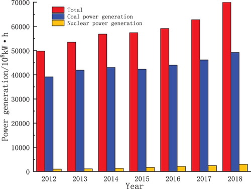
Table 1. Power generation share of wet steam turbine.

Country	Thermal power unit	Nuclear power unit	Total Proportion
USA	63.46%	19.32%	82.78%
China	70.39%	4.21%	74.60%
France	7.1%	71.6%%	78.7%
UK	47.3%	19.4%	66.7%
Russia	63.67%	19.08%	82.75%

The development of steam turbines also keeps pace with the times. One of the main aspects of research regarding wet steam turbines is the mechanism, quantitative evaluation and control measures of the wetness losses (Jiang et al., 2019). Wet steam flow is a two-phase complex flow accompanied by phase transformation and heat and mass transfer. Spontaneous condensation occurs during the high-speed expansion of the steam turbine(Bakhtar & Mohsin, 2014). Thermodynamic and dynamic imbalance, condensation shock, separation and change in the steam flow angle will cause flow loss. The liquid phase is a multi-dispersed phase containing many small droplets of various sizes (Han et al., 2019). The droplets are affected by the viscous force, buoyancy force, virtual mass force, pressure gradient force and Coriolis force in a high-speed steam flow, which renders the research more difficult.

Relevant researches include experimental studies, numerical studies and analytical methods. The analytical method is to integrate the formulas of the nucleation rate and droplet growth rate to obtain the position of the Wilson point and the relationship among the wetness, temperature and expansion rate (Zhang, Wang, Wang, Wu, et al., 2019). Based on the assumption of no slip, Huang and Young (1996) obtained the implicit expressions of the supercooling and expansion rate of the Wilson point by analytic methods and deduced the Wilson point wetness equation. The analytical method and numerical method are complementary, but many flow parameters cannot be simulated simply by function, so the analytical method has some limitations. The measurements of condensation flow parameters were carried out by Petr and Kolovratnik(2014), White and Young (1996), Bakhtar et al. (1995), Yang, Xiang et al. (2017), Qian et al.(2019). The main experimental methods employ micro-video technology, the microwave resonant cavity perturbation method, the optical pulsation method, the ultrasonic method, etc. Because the strong unsteady characteristics, the inflow conditions of the experimental cascade are different from those of a real steam turbine, so it is difficult to measure data accurately, and the measurement work is not easy to carry out (Zhang et al., 2020).

The key to calculate wet steam condensation flow is to establish a reasonable numerical model. Young (1992) considered the centrifugal force and Coriolis force in a rotor cascade and simulated the non-equilibrium condensation flow using real steam thermophysical parameters in a Lagrange coordinate system. White and Hounslow (2000) analyzed the shock structure in condensation flow and discussed the unsteady phenomena caused by condensation. Chandler et al. (2014), Aditya and Prasad (2018), Dykas et al. (2015, 2018), Starzmann et al. (2018), Wang et al. (2018), Yang et al. ( 2019) and others have solved many basic problems, including the shock structure in condensation flow, distribution of condensation parameters, deposition of water droplets and formation mechanism of water films. Better simulation results can be obtained using the real steam equation and two-phase fluid model; however, the slip and temperature difference between phases are often neglected in most existing research. Therefore, the accuracy of numerical simulation can be further improved by using the real steam equation and considering factors such as the velocity slip, energy exchange and mass exchange between two phases.

The condensation will lead to the reduction of turbine efficiency and the damage of blade water erosion. It will also cause shock interference, boundary layer state change and other problems. The existing dehumidification technology of steam turbine includes blade surface heating, steam purging, groove diversion, dehumidification gap, etc. (Han et al., 2018; Zhang, Zhang, Wang, Jin, et al., 2019). The method is to introduce high temperature steam into the cascade cavity. The heat is continuously introduced into the main flow area from the cascade cavity, which makes the water film evaporate and inhibits the nucleation, thus eliminating part of the wetness losses and reducing the number of secondary droplets. However, the existing research is still less, and the mechanism and influencing factors of blade surface heating are not clear. If the heating intensity is too small, the purpose of dehumidification cannot be achieved. However, the economy will be reduced if the heating intensity is too large. Mahpeykar et al. (2014) presented a method to restrain the condensation shock in Laval nozzles by the volumetric heating of the convergent section. Gribin et al. (2014) and Mirhoseini and Boroomand (2017) studied the mechanism of surface heating on condensation flow in a nozzle. Vatanmakan et al. (2018) analyzed the influence of 0 kW/m², 0.5×10⁵ kW/m², 2×10⁵ kW/m², 3.55×10⁵ kW/m² heating intensities in Bakhtar cascade. However, the heating intensity of blade surface is slightly higher. Dehumidification by blade surface heating involves complex phase change heat transfer process. The main steam condenses and emits latent heat, while the water film on the blade surface absorbs heat and evaporates into steam. There are many practical factors affecting the two heat transfer processes. In this paper, the parameter distribution of condensation flow at 0–700 kW/m² heating intensity were investigated using ANSYS CFX 17.0. Moreover, the positive heating intensity region was determined and refined to obtain the best heating condition with higher accuracy.

2. Model establishment

The classical nucleation model is defined as (Bian et al., 2019): (1) $\begin{array}{rl}{J}_{\text{CL}}& =q_c\frac{{{\rho }_g}^2}{{\rho }_l}{\left(\frac{2\sigma }{\pi m^3}\right)}^{1/2}\\ & \times \exp \left(-\frac{4\pi {r_c}^2\sigma }{3k{T}_g}\right)\end{array}$(1)

The critical droplet radius r_c is calculated as (Zhang et al., 2019): (2) $\begin{array}{rl}{r}_c& =\frac{2\sigma }{{\rho }_{l}R{T}_g\ln S}\end{array}$(2) (3) $\begin{array}{rl}S& =\frac{p}{p_S(T_g)}\end{array}$(3)

Wölk modified the Equation (1) by analyzing the experimental data of steam nucleation rate at 220 K-260 K (Wölk et al., 2002). According to the test results, the nucleation rate calculation equation is obtained as: (4) $J_{\text{WS}}=J_{\text{CL}}\exp \left(-27.56+\frac{6.5\times {10}^3}{T_g}\right)$(4)

After using the Wölk modified model, the calculated results still deviate from the experimental values (Starzmann et al., 2018). Bakhtar et al.(1997) indicated that the droplet growth model is also very important for the calculation of condensation flow parameters. The droplet growth rate defined by Gyarmathy (1982) is as: (5) $\begin{array}{rl}\frac{\text{d}r}{\text{d}t}& =\frac{{\lambda }_g\mathrm{\Delta }T(1-(r_c/r))}{{\rho }_l{h}_{fg}r(1+3.18K_{\text{n}})}\end{array}$(5) (6) $\begin{array}{rl}{K}_{\text{n}}& =\frac{\text{3}{\mu }_{\text{1}}\sqrt{R{T}_s}}{4pr}\end{array}$(6)

On this basis, White et al. (1996) made a low-pressure correction of Equation (5): (7) $\begin{array}{rl}\frac{\text{d}r}{\text{d}t}& =\frac{{\lambda }_g\mathrm{\Delta }T(1-(r_c/r))}{{\rho }_l{h}_{fg}r((\text{1}/\text{1 + 1}\text{.5}{K}_{\text{n}})+3.78(1-\delta )(K_{\text{n}}/P_{r\text{g}}))}\end{array}$(7) (8) $\begin{array}{rl}\delta & =\frac{R{T}_S}{h_{fg}}\cdot \left[\phi (p)-0.5-\frac{2-q_c}{\text{2}{q}_c}\cdot \frac{\gamma \text{ + 1}}{\text{2(}\gamma -\text{1)}}\cdot \frac{R{T}_S}{h_{fg}}\right]\end{array}$(8) (9) $\begin{array}{rl}\phi (p)& =3.25\left[1-\tanh \left(\frac{p}{{10}^4}\right)-2\right]\end{array}$(9)

The equation of perfect gas state is defined as: (10) $p={\rho }_{\text{g}}RT(1+B{\rho }_{\text{g}}+C{\rho }_{\text{g}}^{\text{2}})$(10)

The continuity equation is reviewed in by the literature and is calculated as follows (Abadi et al., 2020; Akbarian et al., 2018; Bian et al., 2020; Chen et al., 2019): (11) $\{\begin{array}{l}{\displaystyle \frac{\mathrm{\partial }{\rho }_{\text{g}}}{\mathrm{\partial }t}}+{\displaystyle \frac{\mathrm{\partial }({\rho }_g{u}_j)}{\mathrm{\partial }{x}_j}}=-\dot{m}\\ {\displaystyle \frac{\mathrm{\partial }{\rho }_{\text{d}}}{\mathrm{\partial }t}}+{\displaystyle \frac{\mathrm{\partial }({\rho }_{\text{d}}{u}_{\text{d}j})}{\mathrm{\partial }{x}_j}}=\dot{m}\end{array}$(11)

The volume average density of the liquid phase is as follows: (12) ${\rho }_{\text{d}}={\rho }_{m}Y$(12) The momentum conservation equations for gas and liquid phases are as follows (Hashemian & Lakzian, 2020; Hosseini & Lakzian, 2020; Ramezanizadeh et al., 2019): (13) $\begin{array}{rl}& \frac{\mathrm{\partial }({\rho }_g{u}_i)}{\mathrm{\partial }t}+\frac{\mathrm{\partial }({\rho }_g{u}_i{u}_j)}{\mathrm{\partial }{x}_j}=\frac{\mathrm{\partial }p}{\mathrm{\partial }{x}_i}+\frac{\mathrm{\partial }{\tau }_{ij}}{\mathrm{\partial }{x}_j}+\mathrm{\Delta }\rho g_i-F_{\text{D}}\text{ + }{u}_{i}G\end{array}$(13) (14) $\begin{array}{rl}& \frac{\mathrm{\partial }({\rho }_{\text{d}}{u}_{\text{d}i})}{\mathrm{\partial }t}+\frac{\mathrm{\partial }({\rho }_{\text{d}}{u_{\text{d}}}_i{u}_{\text{d}j})}{\mathrm{\partial }{x}_j}\\ & ={\rho }_{\text{d}}{g}_i+F_{\text{D}}+{\rho }_{\text{m}}\dot{m}({u_{\text{g}}}_i-{u_{\text{d}}}_i)\end{array}$(14)

The energy equation is as follows: (15) $\begin{array}{rl}& \frac{\mathrm{\partial }({\rho }_{g}e)}{\mathrm{\partial }t}+\frac{\mathrm{\partial }({\rho }_g{u}_{j}e)}{\mathrm{\partial }{x}_j}\\ & =\frac{\mathrm{\partial }}{\mathrm{\partial }{x}_i}\left(\lambda \frac{\mathrm{\partial }T}{\mathrm{\partial }{x}_j}\right)-\frac{\mathrm{\partial }(p{u}_j)}{\mathrm{\partial }{x}_j}+\frac{\mathrm{\partial }({\tau }_{kji}{u}_{ki})}{\mathrm{\partial }{x}_j}-\dot{m}(h_t-h_{fg})\end{array}$(15)

If χ = N/Y, the governing equation describing the distribution of droplets is expressed as: (16) $\frac{\mathrm{\partial }({\rho }_{\text{d}}\chi )}{\mathrm{\partial }t}+\frac{\mathrm{\partial }({\rho }_{\text{d}}\chi u_{dj})}{\mathrm{\partial }{x}_j}={\rho }_{g}J$(16) The wetness is defined as: (17) $Y=\frac{4}{3}\pi {\rho }_l{r}^{3}N$(17)

The mass generation rate is defined as: (18) $\dot{m}=4\pi \rho \left[\frac{1}{3}(1-Y)J_{WS}{r_c}^3+{r_c}^{2}N\frac{\text{d}r}{\text{d}t}\right]$(18)

The formula of calculation source term is as follows: (19) $G=1+K\text{n}\left[2.492+0.84\exp \left(-\frac{1.74}{K\text{n}}\right)\right]$(19)

The formula of viscous resistance is as follows: (20) $F_D=\frac{1}{2}{\rho }_{\text{g}}|u_{\text{g}}-u_d|(u_{\text{g}}-u_d)C_{D}A$(20)

3. Calculating preparation instructions

3.1. Physical model construction

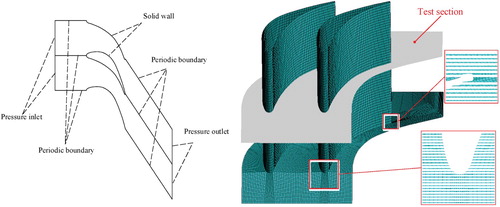
White completed the experimental and numerical study of the condensation flow in a turbine stator cascade earlier, and obtained the complete data of the pressure distribution and the shock wave schlieren figure (White et al., 1996). The data of blade profile are selected from White et al. (1996). The two-dimensional model is based on the assumption that the width of the cascade is infinite, and the influence of the boundary layer near the two sides of the cascade is ignored. The wetness gradient in the boundary layer is decreases rapidly, and close to zero near the blade surface. This is due to the stagnation of the boundary layer on the blade surface, the increase of temperature in the boundary layer and the decrease of subcooling, which make it difficult for spontaneous condensation to occur. This is not completely consistent with the actual situation. In the actual operation of the turbine, due to the deposition and adhesion of the primary water droplets generated by condensation, there will be a water film on the blade surface. Therefore, the boundary layer limits the expansion and condensation of steam flow when only the primary water drop produced by condensation is considered without considering the deposition of water drop. After obtaining the cascade channel model in 2D, the 3D straight cascade model was produced by stretching 300 mm along the vertical direction. Afterwards, the three-dimensional model was divided into regular hexahedron meshes by ANSYS ICEM software, as shown in Figure 2. The calculation area consists of suction surface, pressure surface, hub and shroud, inlet and outlet and periodic boundary. The inlet of cascade is the boundary condition of total pressure inlet, and the outlet of cascade is the boundary condition of pressure outlet. The blade surface, hub and shroud are the boundary condition of wall (Han et al., 2020; Tang et al., 2019; Wen et al., 2019). And the channel part of cascade is the periodic boundary condition. Based on CFX software, the flow field of White cascade is simulated by user-defined function. Because CFX cannot deal with pure two-dimensional problems, it can only import three-dimensional meshes. In this paper, the three-dimensional straight cascade is taken as the research object. The profile of the cascade is identical in different blade height sections. The distribution of cross-section parameters of different blade heights is basically the same, 50% blade height characteristic section is selected for analysis in this paper. The standard k-ε model was selected as the two-phase turbulence model (Starzmann et al., 2018).

Figure 2. Physical modelling.

3.2. Numerical verification

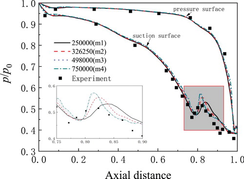
According to White and Young (1996), the L2 case was selected for validation. The inlet steam total pressure and temperature of cascade is 40.9 kPa and 354 K. The outlet pressure of cascade is 19.4 kPa. In order to judge grid quality to the calculation accuracy, the cascade channel was divided into different density grids (250000, 326250, 498000, and 750000). Calculation results of blade surface pressure ratio distribution is shown in Figure 3. Through comparison, it is found that the calculated values of pressure ratio under the four grid numbers are close to the experimental values, which verifies the accuracy of the condensation flow model. The pressure ratio of different density grids only varies between 75% and 90% of the axial chord length of the suction surface of the blade. In order to eliminate the influence of the grids number on the calculation accuracy and shorten the calculation time as much as possible, the physical model with 498000 grid number is selected for calculation in this paper.

Figure 3. Confirmatory comparison (White et al., 1996).

4. Results and discussion

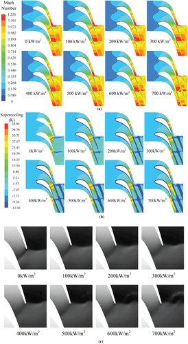
The distributions of the Mach number, supercooling and shock wave in each case are exhibited in Figure 4. With increasing heating intensity, a remarkable change in the Mach number occurs only on the blade surface and near the trailing edge, as shown in Figure 4(a). The Mach number at the throat is about 1.1 and at the outlet is about 1.2. The Mach number distribution is very similar under different conditions. Because the steam condenses in a very short time, the steam flow is reduced. The latent heat of condensation will heats the main steam flow, which resulting in the decrease of velocity and the sudden increase of pressure. Combined with Figure 4(b), the supercooling at the throat reaches the maximum value, and then the spontaneous condensation process occurs rapidly. The steam transits from non-equilibrium state to equilibrium state rapidly, and the supercooling at the downstream of the throat decreases rapidly. The pressure increases after the oblique shock wave. At the cascade outlet, with an increase in heating intensity, the gradient of the Mach number and supercooling at the cascade throat decrease, with a decline in the strength of the condensation shock wave. When it reaches 700 kW/m², the red region is divided. This division is because when the heat flux is too large, the superheated steam area in the blade wake is extremely expanded, and the heat cannot be transmitted in time, resulting in steam blockage and new shock waves, as shown in Figure 4(c).

Figure 4. Distribution of aerodynamic parameters (a) Mach number (b) Supercooling (c) Shock wave.

The aerodynamic parameters for each case are listed in Table 2, and the corresponding variation curves are shown in Figure 5. With the increase of heating, the Mach number at cascade outlet increases first and then decreases, while the total pressure loss coefficient shows the opposite change law. When it reaches 200 kW/m², the aerodynamic parameters reach the optimum value. At this time, compared with the adiabatic case, the Mach number of cascade outlets is 1.0295, which increases by 1.8%, while the total pressure loss coefficient is 0.1004, which decreases by 18.3%. It is not difficult to conclude that the heating intensity, which can make the aerodynamic performance of the cascade reach the optimum state, should be in the range of 100∼300 kW/m².

Figure 5. Aerodynamic performance comparison.

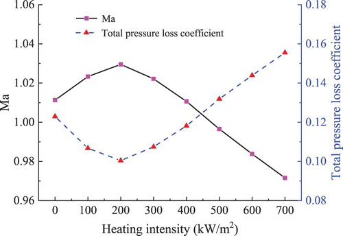
Table 2. Aerodynamic parameters.

Heating intensity (kW/m^2)	0	100	200	300	400	500	600	700
Mach number	1.0113	1.0233	1.0295	1.0222	1.0106	0.9965	0.9838	0.9716
Total pressure loss coefficient	0.1229	0.1068	0.1004	0.1074	0.1182	0.1319	0.1439	0.1555

The distribution of the flow field and liquid phase parameters in each case is shown in Figure 6. According to Figure 6(a), with the increase of heating, the red region (high wetness) decreases gradually, accompanied by the expansion of the blue region (low wetness) close to the trailing edge. Under heating conditions, the nucleation rate on the blade surface is reduced to zero due to the existence of superheated steam on the blade surface. With increasing heating intensity, the peak nucleation rate decreases, but the area of the nucleation region expands and approaches the cascade exit, as shown in Figure 6(b). Due to the addition of heat, the unbalance of steam in the expansion process is weakened, and the condensation is delayed. In addition, an increase in overall steam temperature inhibits the growth of water droplets and reduces the number and diameter of water droplets in the flow field, as shown in Figure 6(c and d). Table 3 gives the liquid parameters at the outlet. According to the data in the table, heating the blade surface can effectively control the outlet liquid parameters. However, when the heating intensity reaches 400 kW/m², it is not helpful or even negative to increase the heating intensity to improve the steam wetness control effect. Therefore, improving the heating intensity can optimize the dehumidification performance of the cascade, but not blindly.

Figure 6. Distribution of the condensation parameter (a) Wetness (b) Nucleation rate (c) Droplet number (d) Droplet diameter.

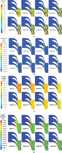
Table 3. Liquid parameters.

Heating intensity (kW/m^2)	0	100	200	300	400	500	600	700
Wetness (%)	2.7737	1.8208	1.3079	1.0855	1.0075	0.9528	0.9440	0.9663
Droplet number (×10^17)	3.5413	2.0432	1.1175	0.4377	0.5219	0.6187	0.8250	0.2724
Droplet diameter (×10^−8 m)	2.7349	2.7175	2.4736	2.7071	2.3269	2.1412	1.8032	2.7184

The values of the enthalpy drop and entropy increase for each case are listed in Table 4. The corresponding curves, together with the average wetness at cascade outlet, are shown in Figure 7. When it is lower than 200 kW/m², the average wetness at the cascade outlet decreases greatly, while the enthalpy drop and entropy increase change in the opposite direction, but their variation ranges are small in general. When it is greater than 200 kW/m², the average wetness at the cascade outlet decreases slowly, while the entropy increase increases almost linearly with a larger slope, and the steam enthalpy drop decreases linearly as well. When it reaches 400 kW/m², the enthalpy drop is negative, and the performance of steam is not positive, accompanied by a large irreversible loss. Under all heating conditions, the 100 kW/m² can make the comprehensive performance relatively optimal. Compared with the 0 kW/m² condition, the enthalpy drop increases by 1%, the entropy increase decrease by 1.4%, and the wetness decrease by 0.953%. In view of the changing characteristics of the three curves, the optimum heating intensity, which can improve the steam performance and reduce the overall irreversible loss, should exist in the range of 0–200 kW/m². However, only a few cases were calculated in this range, so the following article will refine the range and determine the optimum heating condition.

Figure 7. Comprehensive analysis.

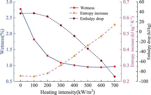
Table 4. Performance parameter comparison.

Heating intensity (kW/m^2)	0	100	200	300	400	500	600	700
Enthalpy drop (kJ/kg)	36.832	37.194	30.641	12.896	−8.545	−34.131	−58.194	−90.328
Entropy increase (kJ·kg^−1·K^−1)	0.2344	0.2311	0.2503	0.3013	0.3600	0.4258	0.4840	0.5564

The effect of wet steam on stage efficiency can be evaluated by the Baumann (1912). Baumann formula indicates that the average wetness of outlet increases by 1%, and the stage efficiency decreases by 1%. To better distinguish the variation trend of the steam parameters with heating intensity, the range of 0–200 kW/m² was divided into 10 equal parts, and the corresponding numerical calculation was carried out in this section. The corresponding values of the 5 evaluation parameters for the 11 heating conditions are shown in Table 5, and Figure 8 shows the parameters in the form of curves. According to Figure 8(a), when the heating intensity reaches 120 kW/m², a noteworthy decline appears in the change speed of these two parameters. According to Figure 8(b), increasing the heating intensity reduces the decreasing speed of the outlet average wetness. Due to the addition of heat, the overall parameter of the steam flow field is raised, i.e. the heat transfer efficiency will be reduced if the heat is continued to be introduced. With increasing heating intensity, the enthalpy drop first decreases and rebounds with a heating intensity of 20 kW/m². When it reaches 120 kW/m², the enthalpy drop obtains its maximum value and then decreases at an increasing rate. The change trend of the entropy increase curve is basically opposite to that of the enthalpy drop curve. The entropy increase reaches a minimum 0.2303 kJ·kg⁻¹·K⁻¹. Under unheated condition, the entropy increase of liquid phase is greater than that of vapor phase. However, with the increase of heating intensity, the steam near the blade surface no longer condenses and the wetness decreases. Therefore, when it is less than 120 kW/m², the local entropy increase will decreases with the raise of heating. This is mainly due to the elimination of entropy increase of the liquid phase.

Figure 8. Comprehensive performance evaluation (a) Aerodynamic performance evaluation (b) Overall loss and dehumidification performance evaluation.

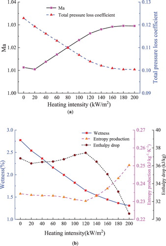
Table 5. Comprehensive evaluation parameters.

Heating intensity (kW/m^2)	Wetness (%)	Entropy increase (kJ·kg^−1·K^−1)	Enthalpy drop (kJ/kg)	Total pressure loss coefficient	Mach number
0	2.7737	0.2344	36.8321	0.1229	1.0113
20	2.5398	0.2336	36.2663	0.1193	1.0105
40	2.3623	0.2333	36.4182	0.1161	1.0138
60	2.1614	0.2332	36.4747	0.1130	1.0170
80	1.9949	0.2325	36.7325	0.1099	1.0202
100	1.8208	0.2311	37.1943	0.1068	1.0233
120	1.6471	0.2303	37.4513	0.1039	1.0262
140	1.5374	0.2331	36.4620	0.1021	1.0280
160	1.4449	0.2373	35.0627	0.1010	1.0292
180	1.3639	0.2430	33.1047	0.1004	1.0296
200	1.3079	0.2503	30.6406	0.1004	1.0295

Generally, the evaluation parameters of the 120 kW/m² are positive. The wetness, entropy increase and total pressure loss coefficient are 1.6471%, 0.2303 kJ·kg⁻¹·K⁻¹ and 0.1039, which are 1.1266%, 1.7% and 15.5% lower than those under the adiabatic condition, respectively. The enthalpy drop and Mach number are 37.4513 kJ/kg and 1.0262, which are 1.7% and 1.5% higher than that of the adiabatic case, respectively. Therefore, choosing appropriate heating intensity can reduce the wetness losses and water erosion damage. Under different conditions, the coupling relationship between entropy increase and heating intensity is the focus of further research.

5. Conclusions

In this paper, a two-phase fluid model was used to evaluate the influence of blade surface heating intensity on cascade aerodynamic performance, dehumidification performance and energy loss. The main conclusions are as follows:

1. Compared with the adiabatic case, the outlet Mach number of 200 kW/m² heating intensity is 1.0295, which increases by 1.8%, while the total pressure loss coefficient is 0.1004, which decreases by 18.3%. The excessive heating intensity will lead to the formation of a new shock wave, which seriously hinders the steam flow.

2. Compared with the adiabatic case, the outlet wetness of 200 kW/m² heating intensity decreases by 1.4658%, while the droplet number decreases by 31.556%. Heating the blade surface can effectively reduce the wetness and the droplet diameter.

3. At the initial stage of applying heat to the blade, the steam wetness decreases rapidly, an increase appears in the enthalpy drop, the entropy increase experiences a decline. When it is greater than 200 kW/m², the wetness decreases slowly, while the enthalpy drop falls rapidly, and the entropy increase rises steeply. The optimum heating intensity is 120 kW/m².

In this paper, several surface heating schemes of stator cascade blade are given, and the influence of different heating intensity on condensation flow is obtained. However, the heating scheme is relatively simple, and the whole blade surface is uniformly heated. In the follow-up study, the cascade will be divided into several regions, and only the key parts will be heated. On this basis, the optimal region coupling heating scheme will be obtained. In addition, an experimental platform will be built to verify the accuracy of the calculation by carrying out relevant blade surface heating experiments.

Nomenclature

A	=	windward area,(m2)
CD	=	drag force coefficient
e	=	energy density, (kJ·kg–1·m–3)
FD	=	viscous resistance (N)
G	=	calculation source term
gi	=	gravitational acceleration(m·s–2)
ht	=	total enthalpy (kJ·kg–1)
hfg	=	condensation latent heat (kJ·kg–1)
J	=	nucleation rate (m3·s)–1
JCL	=	nucleation rate by classical nucleation model (m3·s)–1
JWS	=	nucleation rate by Wölk model (m3·s)–1
k	=	Boltzmann constant
Kn	=	Knudsen number
m	=	single molecular mass (kg)
$\dot{m}$	=	mass generation rate (kg·s–1)
Ma	=	Mach number
N	=	amount of droplets (m–3)
p	=	pressure (Pa)
Prg	=	Prandtl number
qc	=	condensation coefficient
r	=	droplet radius (m)
R	=	gas constant (J·(kg·K)–1)
rc	=	critical droplet radius (m)
S	=	supersaturation ratio
T	=	temperature (K)
TS	=	saturation temperature
ΔT	=	degree of supercooling (K)
u	=	velocity component (m·s–1)
Y	=	wetness
γ	=	gas adiabatic constant
δ	=	semi-empirical correction coefficient
λg	=	thermal conductivity of gas (W·(m·K)–1)
μ1	=	coefficient of laminar viscosity
ρ	=	density (kg·m–3)
σ	=	liquid surface tension (N·m–1)
ϕ(P)	=	correction coefficient of droplet growth model

Subscript

d	=	volume average parameter
m	=	mixed phase parameter
g	=	gas
l	=	liquid
S	=	saturation state

Acknowledgements

The authors are thankful for the support provided by the Natural Science Foundation of Hebei Province, China (grant number E2020502001), and the Fundamental Research Funds for the Central Universities of China (grant number 2019MS092), the National Science and Technology Support Program of China (grant number 2014BAA06B01).

Disclosure statement

No potential conflict of interest was reported by the author(s).

Additional information

Funding

The authors are thankful for the support provided by the Natural Science Foundation of Hebei Province, China [grant number E2020502001], and the Fundamental Research Funds for the Central Universities of China [grant number 2019MS092], the National Science and Technology Support Program of China [grant number 2014BAA06B01].

References

- Abadi, A. M. E., Sadi, M., Farzaneh-Gord, M., Ahmadi, M. H., & Chau, K. W. (2020). A numerical and experimental study on the energy efficiency of a regenerative heat and mass exchanger utilizing the counter-flow maisotsenko cycle. Engineering Applications of Computational Fluid Mechanics, 14(1), 1–12. https://doi.org/10.1080/19942060.2019.1617193
- Aditya, P., & Prasad, B. (2018). Effect of wall surface roughness on condensation shock. International Journal of Thermal Science, 132, 435–445. https://doi.org/10.1016/j.ijthermalsci.2018.06.028
- Akbarian, E., Najafi, B., Jafari, M., Ardabili, S. F., & Chau, K. W. (2018). Experimental and cfd-based numerical simulation of using natural gas in a dual-fuelled diesel engine. Engineering Applications of Computational Fluid Mechanics, 12(1), 517–534. https://doi.org/10.1080/19942060.2018.1472670
- Bakhtar, F., Ebrahimi, M., & Bamkole, B. (1995). On the performance of a cascade of turbine rotor tip section blading in nucleating steam: Part 2: Wake traverses. Proceedings of the Institution of Mechanical Engineers, Part C: Journal of Mechanical Engineering Science, 209(33), 169–177. https://doi.org/10.1243/PIME_PROC_1995_209_140_02
- Bakhtar, F., Mashmoushy, H., & Buckley, J. R. (1997). On the performance of a cascade of turbine rotor tip section blading in wet steam part 1: Generation of wet steam of prescribed droplet sizes. Proceedings of the Institution of Mechanical Engineers, Part C: Journal of Mechanical Engineering Science, 211(7), 519–529. https://doi.org/10.1243/0954406971521908
- Bakhtar, F., & Mohsin, R. (2014). A study of the throughflow of nucleating steam in a turbine stage by a time-marching method. Proceedings of the Institution of Mechanical Engineers Part C-Journal of Mechanical Engineering Science, 228(5), 932–949. https://doi.org/10.1177/0954406213490873
- Baumann, K. (1912). Recent developments in steam turbine practice. Journal of the Institution of Electrical Engineers, 48(213), 768–842. https://doi.org/10.1049/jiee-1.1912.0035
- Bian, J., Cao, X., Yang, W., Guo, D., & Xiang, C. (2020). Prediction of supersonic condensation process of methane gas considering real gas effects. Applied Thermal Engineering, 164. https://doi.org/10.1016/j.applthermaleng.2019.114508
- Bian, J., Cao, X., Yang, W., Song, X., Xiang, C., & Gao, S. (2019). Condensation characteristics of natural gas in the supersonic liquefaction process. Energy, 168, 99–110. https://doi.org/10.1016/j.energy.2018.11.102
- Chandler, K., White, A. J., & Young, J. B. (2014). Non-equilibrium wet-steam calculations of unsteady low-pressure turbine flows. Proceedings of the Institution of Mechanical Engineers, Part A: Journal of Power and Energy, 228(2), 143–152. https://doi.org/10.1177/0957650913511802
- Chen, Y., Hu, Y., & Zhang, S. (2019). Structure optimization of submerged water jet cavitating nozzle with a hybrid algorithm. Engineering Applications of Computational Fluid Mechanics, 13(1), 591–608. https://doi.org/10.1080/19942060.2019.1628106
- Dykas, S., Majkut, M., Smolka, K., & Strozik, M. (2018). An attempt to make a reliable assessment of the wet steam flow field in the de laval nozzle. Heat and Mass Transfer, 54(9), 2675–2681. https://doi.org/10.1007/s00231-018-2313-7
- Dykas, S., Majkut, M., Strozik, M., & Smolka, K. (2015). Losses estimation in transonic wet steam flow through linear blade cascade. Journal of Thermal Science, 24(2), 109–116. https://doi.org/10.1007/s11630-015-0762-6
- Gribin, V., Tishchenko, A., Tishchenko, V., Gavrilov, I., Khomiakov, S., & Popov, V. (2014). An experimental study of influence of the steam injection on the profile surface on the turbine nozzle cascade performance. Asme Turbo Expo: Turbine Technical Conference & Exposition. https://doi.org/10.1115/GT2014-27118
- Gyarmathy, G. (1982). The spherical droplet in gaseous carrier streams: Review and synthesis. Multiphase Science and Technology, 1(1-4), 99–279. https://doi.org/10.1615/MultScienTechn.v1.i1-4.20
- Han, X., Zeng, W., & Han, Z. (2019). Investigation of the comprehensive performance of turbine stator cascades with heating endwall fences. Energy, 174, 1188–1199. https://doi.org/10.1016/j.energy.2019.03.038
- Han, X., Zeng, W., & Han, Z. (2020). Investigating the dehumidification characteristics of the low-pressure stage with blade surface heating. Applied Thermal Engineering, 164. https://doi.org/10.1016/j.applthermaleng.2019.114538
- Han, X., Zeng, W., Han, Z., Li, P., & Qian, J. (2019). Effect of the nonaxisymmetric endwall on wet steam condensation flow in a stator cascade. Energy Science & Engineering, 7(2), 557–572. https://doi.org/10.1002/ese3.298
- Han, Z., Zeng, W., Han, X., & Xiang, P. (2018). Investigating the dehumidification characteristics of turbine stator cascades with parallel channels. Energies, 11(9), 2306. https://doi.org/10.3390/en11092306
- Hashemian, A., & Lakzian, E. (2020). On the application of isogeometric finite volume method in numerical analysis of wet-steam flow through turbine cascades. Computers & Mathematics with Applications, 79(6), 1687–1705. https://doi.org/10.1016/j.camwa.2019.09.025
- Hosseini, R., & Lakzian, E. (2020). Optimization volumetric heating in condensing steam flow by a novel method. Journal of Thermal Analysis and Calorimetry, 140(5), 2421–2433. https://doi.org/10.1007/s10973-019-09001-1
- Huang, L., & Young, J. B. (1996). An analytical solution for the Wilson point in homogeneously nucleating flows. Proceedings of the Royal Society A-Mathematical Physical and Engineering Sciences, 452(1949), 1459–1473. https://doi.org/10.1098/rspa.1996.0074
- Jiang, X., Lin, A., Malik, A., Chang, X., & Xu, Y. (2019). Numerical investigation on aerodynamic characteristics of exhaust passage with consideration of multi-factor components in a supercritical steam turbine. Applied Thermal Engineering, 162. https://doi.org/10.1016/j.applthermaleng.2019.114085
- Mahpeykar, M. R., Rad, E. A., & Teymourtash, A. R. (2014). Analytical investigation into simultaneous effects of friction and heating on a supersonic nucleating laval nozzle. Scientia Iranica, 21(5), 1700–1708.
- Mirhoseini, M. S., & Boroomand, M. (2017). Multi-objective optimization of hot steam injection variables to control wetness parameters of steam flow within nozzles. Energy, 141, 1027–1037. https://doi.org/10.1016/j.energy.2017.09.138
- Petr, V., & Kolovratnik, M. (2014). The assessment of the effect of binary homogeneous nucleation on wet steam energy loss in a low pressure steam turbine. Proceedings of the Institution of Mechanical Engineers Part A-Journal of Power and Energy, 228(5), 525–535. https://doi.org/10.1177/0957650914531947
- Qian, J., Gu, Q., Yao, H., & Zeng, W. (2019). Dielectric properties of wet steam based on a double relaxation time model. The European Physical Journal E, 42(2), 22. https://doi.org/10.1140/epje/i2019-11783-1
- Ramezanizadeh, M., Alhuyi Nazari, M., Ahmadi, M. H., & Chau, K. W. (2019). Experimental and numerical analysis of a nanofluidic thermosyphon heat exchanger. Engineering Applications of Computational Fluid Mechanics, 13(1), 40–47. https://doi.org/10.1080/19942060.2018.1518272
- Starzmann, J., Hughes, F. R., Schuster, S., White, A. J., Halama, J., Hric, V., Kolovratník, M., Lee, H., Sova, L., Št’astný, M., Grübel, M., Schatz, M., Vogt, D. M., Patel, Y., Patel, G., Turunen-Saaresti, T., Gribin, V., Tishchenko, V., Gavrilov, I., … Li, L. (2018). Results of the international wet steam modeling project. Proceedings of the Institution of Mechanical Engineers Part A Journal of Power & Energy, 232(5), 550–570. https://doi.org/10.1177/0957650918758779
- Tang, Y., Liu, Z., Li, Y., Shi, C., & Lv, C. (2019). A combined pressure regulation technology with multi-optimization of the entrainment passage for performance improvement of the steam ejector in MED-TVC desalination system. Energy, 175, 46–57. https://doi.org/10.1016/j.energy.2019.03.072
- Tang, Y., Liu, Z., Li, Y., Wu, H., Zhang, X., & Yang, N. (2019). Visualization experimental study of the condensing flow regime in the transonic mixing process of desalination-oriented steam ejector. Energy Conversion and Management, 197. https://doi.org/10.1016/j.enconman.2019.111849
- Vatanmakan, M., Lakzian, E., & Mahpeykar, M. R. (2018). Investigating the entropy generation in condensing steam flow in turbine blades with volumetric heating. Energy, 147, 701–714. https://doi.org/10.1016/j.energy.2018.01.097
- Wang, C., Wang, X., & Ding, H. (2018). Boundary layer of non-equilibrium condensing steam flow in a supersonic nozzle. Applied Thermal Engineering, 129, 389–402. https://doi.org/10.1016/j.applthermaleng.2017.10.015
- Wen, C., Karvounis, N., Wahher, J. H., Yan, Y., Feng, Y., & Yang, Y. (2019). An efficient approach to separate CO2 using supersonic flows for carbon capture and storage. Applied Energy, 238, 311–319. https://doi.org/10.1016/j.apenergy.2019.01.062
- White, A. J., & Hounslow, M. J. (2000). Modelling droplet size distributions in polydispersed wet-steam flows. International Journal of Heat and Mass Transfer, 43(11), 1873–1884. https://doi.org/10.1016/S0017-9310(99)00273-2
- White, A. J., Young, J. B., & Walters, P. T. (1996). Experimental validation of condensing flow theory for a stationary cascade of steam turbine blades. Philosophical Transactions of the Royal Society A: Mathematical, Physical and Engineering Sciences, 354(1704), 59–88. https://doi.org/10.1098/rsta.1996.0003
- Wölk, J., Strey, R., Heath, C. H., & Wyslouzil, B. E. (2002). Empirical function for homogeneous water nucleation rates. The Journal of Chemical Physics, 117(10), 4954–4960. https://doi.org/10.1063/1.1498465
- Yang, B., Xiang, Y., Cai, X., Zhou, W., Liu, H., Li, S., Gao, W. (2017). Simultaneous measurements of fine and coarse droplets of wet steam in a 330 MW steam turbine by using imaging method. Proceedings of the Institution of Mechanical Engineers Part A Journal of Power and Energy, 231(3), 161–172. https://doi.org/10.1177/0957650916685910
- Yang, Y., Zhu, X., Yan, Y., Ding, H., & Wen, C. (2019). Performance of supersonic steam ejectors considering the nonequilibrium condensation phenomenon for efficient energy utilisation. Applied Energy, 242, 157–167. https://doi.org/10.1016/j.apenergy.2019.03.023
- Young, J. B. (1992). Two-dimensional, nonequilibrium, wet-steam calculations for nozzles and turbine cascades. Journal of Turbomachinery, 114(3), 569–579. https://doi.org/10.1115/1.2929181
- Zhang, G., Dykas, S., Yang, S., Zhang, X., & Wang, J. (2020). Optimization of the primary nozzle based on a modified condensation model in a steam ejector. Applied Thermal Engineering, 171. https://doi.org/10.1016/j.applthermaleng.2020.115090
- Zhang, G., Wang, F., Wang, D., Wu, T., Qin, X., & Jin, Z. (2019). Numerical study of the dehumidification structure optimization based on the modified model. Energy Conversion and Management, 181, 159–177. https://doi.org/10.1016/j.enconman.2018.12.001
- Zhang, G., Zhang, X., Wang, D., Jin, Z., & Qin, X. (2019). Performance evaluation and operation optimization of the steam ejector based on modified model. Applied Thermal Engineering, 163. https://doi.org/10.1016/j.applthermaleng.2019.114388