Vortex identification and evolution of a jet in cross flow based on Rortex

Abstract

Jet in cross flow is an important issue in engineering practice, for example, it is used to improve turbine efficiency in film cooling. In this study, the large eddy simulation and the spectrum analysis are employed to analyze the vortices in a jet in cross flow. The results show that the Rortex method more accurately identifies the vortex structures than other methods. In the analysis of the evolution of the spatial vortex structures, it is affirmed that the spectrum analysis using the Rortex value can effectively identify the characteristic vortex structures in a jet in cross flow.

KEYWORDS:

• Vortex
• Rortex
• spectrum analysis
• dominant frequency
• jet in cross flow

1. Introduction

Mixing processes in a jet in cross flow (JICF) (Margason, 1993) (in which a jet is injected into a uniform free stream) are of fundamental importance in engineering practice such as pollutant formation, chemical reactions and film-cooling. In early numerical investigations of the JICF, vortex methods (Coelho & Hunt, 1989; Cortelezzi & Karagozian, 2001; Margason, 1970) and Reynolds-averaged Navier-Stokes method (Demuren, 1993; Sykes et al., 1986) had been applied with rough vortex identification. Recently, JICF was studied carefully using the large eddy simulation (LES). The effect of counter-rotating vortex pair (CRVP) was investigated of a round jet in cross-flow (Yuan et al., 1999). And the evolution of mean velocities, resolved Reynolds stresses, and turbulent kinetic energy along the centre line were also analysed. The momentum and scalar fields of LES were compared with the second order turbulence closure calculations (Mengler et al., 2001). The detailed of the flow topologies and turbulence scales in the jet-in-cross-flow were presented using LES with a highly resolved grid and well controlled boundary conditions (Ruiz et al., 2015). Direct numerical simulation method (Grout et al., 2011; Muppidi & Mahesh, 2007) was also employed to investigate the mechanism of JICF.

In the engineering applications, the efficiency and optimization of mixing processes has been strongly investigated. For example, film-cooling technology has been wildly used in combustion chamber and turbine blade to isolate hot gas and protect the surface (Goldstein, 1971). However, the physics of the mixing processes are extremely complex. In the downstream of a single row of film cooling holes, the cooling effectiveness drops due to the mixing of mainstream and coolant flow. Meanwhile, most of the film cooling correlations in published literatures were mostly focus on the blowing ratio (BR), inclined angel, the shape of the hole and so on (Goldstein et al., 1974; Gritsch et al., 1998; Hasan et al., 2003; Heidmann & Ekkad, 2008; Islami & Jubran, 2012; Islami et al., 2010; Khajehhasani & Jubran, 2016; Ming Li & Hassan, 2015; Yuen & Martinez-Botas, 2003). In the film cooling process, abundant vortex structures are generated and transported owing to the interaction between the jet flow and the cross flow (Kelso et al., 1996). The generation and transportation of vortices affect the heat and material exchange. The results of a spectral analysis indicated a high correlation between the shedding period of the CRVP and the film-cooling effectiveness (Chen et al., 2020). Thus, further investigations of the vortex effect in the jet in cross flow process are in great demand to help to predict the cooling effectiveness distributions (Ekkad & Han, 2013).

In previous studies, many vortex visualization methods (Chong et al., 1990; Hunt et al., 1988; Jeong & Hussain, 1995; Zhou et al., 1999) are proposed based on the velocity gradient tensor. Differ from these methods, Liu and his collaborators proposed a novel method, Rortex (Gao & Liu, 2019; Liu et al., 2018; Tian et al., 2018). The Rortex method makes it definite physical meaning by different decomposition of the velocity gradient tensor (Sun, 2019; Vaclav, 2007). Zhan et al. (2019) proved that Rortex has better advantages than Q criterion in hydraulic engineering application. In the current study, four methods, Rortex, Q criterion, Lambda-2 criterion and swirling strength are chosen to visualize the vortex structures. Spectrum analysis is employed to determine the generation frequency of vortex.

2. Models and configuration

The eigenvalues ($\lambda$) of the velocity gradient tensor ($\mathrm{\nabla }\overrightarrow{v}$) satisfies the following equation: (1) ${\lambda }^3+P{\lambda }^2+Q\lambda +T\text{ = }0$(1) Here, P, Q and T are three invariants of the velocity gradient tensor. The velocity gradient tensor can be decomposed into two parts as follows: (2) $\mathrm{\nabla }\overrightarrow{v}=\frac{1}{2}(\mathrm{\nabla }\overrightarrow{v}+\mathrm{\nabla }{\overrightarrow{v}}^T)+\frac{1}{2}(\mathrm{\nabla }\overrightarrow{v}-\mathrm{\nabla }{\overrightarrow{v}}^T)=S+\mathrm{\Omega }$(2) Here $S$ is the symmetric part known as the rate of strain and $\mathrm{\Omega }$ is the anti-symmetric part known as the vorticity tensor.

The Q criterion (Hunt et al., 1988) is directly derived as follows: (3) $Q=\frac{1}{2}(||\mathrm{\Omega }|{|}_{}^2-||S|{|}_{}^2)$(3) The Q criterion defines Q > 0 to represent the existence of a vortex. In other words, the vorticity magnitude is greater than the magnitude of the rate of strain in the vortices areas.

If the unsteady and viscous terms in the incompressible Navier-Stokes equation are ignored, then $S^2+{\mathrm{\Omega }}^2=-\mathrm{\nabla }(\mathrm{\nabla }p)/\rho$. Here $p$ is pressure and $\rho$ is density. The Lambda-2 criterion (Jeong & Hussain, 1995) is defined as the second largest eigenvalue ${\sigma }_2$ of $S^2+{\mathrm{\Omega }}^2$ with ${\sigma }_2<0$. When there are two negative eigenvalues, the pressure is a minimum in the plane formed by the corresponding eigenvectors of these two negative eigenvalues.

If Equation (1) has complex eigenvalues, then the velocity gradient tensor can be decomposed as follows: (4) $\mathrm{\nabla }\overrightarrow{v}=[{\nu }_r{\nu }_{cr}{\nu }_{ci}]\left[\begin{array}{ccc}{\lambda }_r& 0& 0\\ 0& {\lambda }_{cr}& {\lambda }_{ci}\\ 0& -{\lambda }_{ci}& {\lambda }_{cr}\end{array}\right][{\nu }_r{\nu }_{cr}{\nu }_{ci}{]}^{-1}$(4) Here ${\lambda }_r,{\lambda }_{cr}\pm i{\lambda }_{ci}$ are eigenvalues, ${\nu }_r,{\nu }_{cr}\pm i{\nu }_{ci}$ are the corresponding eigenvectors. Swirling strength (Zhou et al., 1999) is defined as ${\lambda }_{ci}$, since it represents an instantaneous angular velocity in the local surface coordinate system formed by the three eigenvectors.

Rortex (Liu et al., 2018) represents the local fluid rotation. In the Rortex method, By applying a coordinate rotation A (Equation (6)), the rotation axis in the local coordinate system is the Z axis, and the rotation intensity can be obtained in the local coordinate system (Equation (7)). (5) $\begin{array}{rl}\mathrm{\nabla }\overrightarrow{v}\cdot \overrightarrow{r}& ={\lambda }_r\overrightarrow{r}\end{array}$(5) (6) $\begin{array}{rl}\mathrm{\nabla }\overrightarrow{V}& =\mathrm{A}\mathrm{\nabla }\overrightarrow{v}{A}^T=\left[\begin{array}{ccc}{\displaystyle \frac{\mathrm{\partial }U}{\mathrm{\partial }X}}& {\displaystyle \frac{\mathrm{\partial }U}{\mathrm{\partial }Y}}& 0\\ {\displaystyle \frac{\mathrm{\partial }V}{\mathrm{\partial }X}}& {\displaystyle \frac{\mathrm{\partial }V}{\mathrm{\partial }Y}}& 0\\ {\displaystyle \frac{\mathrm{\partial }W}{\mathrm{\partial }X}}& {\displaystyle \frac{\mathrm{\partial }W}{\mathrm{\partial }Y}}& {\displaystyle \frac{\mathrm{\partial }W}{\mathrm{\partial }Z}}\end{array}\right]\end{array}$(6) (7) $\begin{array}{rl}R& =\{\begin{array}{ll}2(\beta -\alpha ),& {\alpha }^2-{\beta }^2<0\\ 0,& {\alpha }^2-{\beta }^2\ge 0\end{array}\\ \alpha & ={\displaystyle \frac{1}{2}}\sqrt{{\left({\displaystyle \frac{\mathrm{\partial }V}{\mathrm{\partial }Y}}-{\displaystyle \frac{\mathrm{\partial }U}{\mathrm{\partial }X}}\right)}^2+{\left({\displaystyle \frac{\mathrm{\partial }V}{\mathrm{\partial }X}}+\frac{\mathrm{\partial }U}{\mathrm{\partial }Y}\right)}^2}\\ \beta & =\frac{1}{2}\left(\frac{\mathrm{\partial }V}{\mathrm{\partial }X}-\frac{\mathrm{\partial }U}{\mathrm{\partial }Y}\right)\\ \overrightarrow{R}& =R\overrightarrow{r}\end{array}$(7)

The BR is defined as follows: (8) $BR={\rho }_c{u}_c/{\rho }_{\mathrm{\infty }}{u}_{\mathrm{\infty }}$(8) Here $u_c^{}$ represents the coolant jet velocity, $u_{\mathrm{\infty }}^{}$ represents the cross-flow velocity, and ${\rho }_c$ and ${\rho }_{\mathrm{\infty }}$ represent the jet flow and cross-flow densities, respectively.

The film-cooling effectiveness is scaled by temperature and is defined as follows: (9) $\eta =(T_{ad,w}-T_{\mathrm{\infty }})/(T_c-T_{\mathrm{\infty }})$(9) Here $T_{ad,w}$ represents the adiabatic wall temperature, $T_c$ represents the coolant jet flow temperature, and $T_{\mathrm{\infty }}$ represents the hot cross-flow temperature.

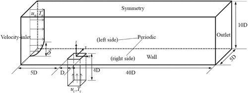
Figure 1 shows the configuration and boundary conditions of the simulation. Base on the square jet diameter and the cross-flow velocity, the Reynolds number, $\mathrm{Re}=\rho u_{\mathrm{\infty }}/D$ is approximate 9300, where D = 12.7 mm is the diameter of the square jet hole.

Figure 1. Computational domain and the boundary conditions.

The numerical simulation is performed using ANSYS Fluent 15.0. The LES Smagorinsky-Lilly model with constant C_s = 0.1 is employed as the turbulence model with SIMPLE (Semi-Implicit Method for Pressure Linked Equations) as the pressure-velocity coupling algorithm. Pressure interpolation, convection and viscous discretization schemes are all second order. Time discretization scheme is bounded second-order implicit. The relaxation factor of pressure is 0.5, the relaxation factor of density is 1, the relaxation factor of body force is 1, and the relaxation factor of momentum is 0.6. To ensure that the Courant number is less than 1.0, the non-dimensional time step is set to approximate $0.17D/u_{\mathrm{\infty }}$. Statistical data sampling were obtained over a period of $90000D/u_{\mathrm{\infty }}$ when the statistically steady state has been reached. The velocity profile with a boundary layer at the inlet boundary is obtained in a straight channel numerical simulation without the jet hole. The Rortex, Q criterion, Lambda-2 criterion and swirling strength are calculated using User Defined Functions.

3. Validation

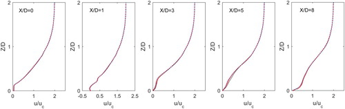
The grid independence test is conducted for the case with a BR of 0.5. Three different meshes are selected for comparison: mesh 1 with averaged y+ = 2.40, mesh 2 with averaged y+ = 1.59 and mesh 3 with averaged y+ = 0.72. All the three meshes have approximately 5,000,000 cells. Figure 2 shows the time-averaged streamwise velocity profiles calculated using the three meshes. The calculated velocity profiles are similar for the mesh 2 and mesh 3, while the velocity profiles of mesh 1 have differences near the wall region at X/D = 3, X/D = 5 and X/D=8. Therefore, mesh 2, with approximately 5,000,000 grid cells and averaged y+ = 1.59 is selected for the subsequent simulations.

Figure 2. Grid independence test, mesh 1 (-), mesh 2 (·), mesh 3 (-).

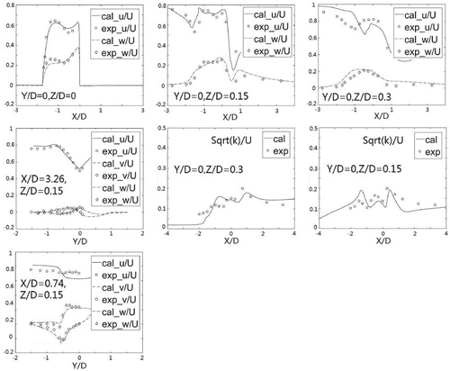
The validation of the numerical simulation is verified by comparing with the experimental results. Figure 3 shows film-cooling effectiveness of Kohli and Bogard (1997), and Figure 4 shows the velocity and turbulence profiles of Pietrzyk et al. (1989). The film-cooling effectiveness is a little lower near the jet hole because of the shedding of the vortex. The velocity profiles are in good agreement with the experimental measurements, except in the u direction of the line (Y/D = 0, Z/D = 0.3), which may be due to the interaction between the jet flow and the cross flow. Therefore, the LES with dynamic Smagorinsky-Lilly subgrid-scale model is reliable.

Figure 3. Comparison of the experimental measurements of Kohli and Bogard (1997) with the film cooling effectiveness from the numerical simulations at (a) BR = 0.5, (b) BR = 1.5.

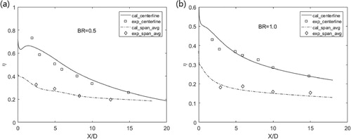
Figure 4. Comparison of the experimental measurements of Pietrzyk et al. (1989) with velocity and turbulence profiles from the numerical simulations at BR = 0.5.

4. Results and discussion

4.1. Comparison of vortex identification methods

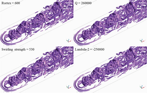
Extracting the values of Rortex, Q criterion, Lambda-2 criterion and swirling strength of each cell in the case, plotting them in the X-Y frame, we can obtain the correlation between Rortex and the other three quantities, as shown in Figure 5. The fitting method is polynomial. For the correlation of Rortex – Q criterion and Rortex – Lambda-2 criterion, cubic polynomial has the best effect; for the correlation of Rortex – swirling strength, quadratic polynomial is the best. As can be seen from Figure 5, Rortex has a highest correlation with swirling strength, followed by Q criterion, and Lambda-2 criterion is the last. According to the fitting formulas in Figure 5, the values of the other three methods corresponding to the determined Rortex value can be obtained, as shown in Table 1. In the following text, we choose Rortex = 300 for BR = 0.1 and Rortex = 600 for BR = 0.5 to visualize the vortex structures.

Figure 5. The correlation between Rortex and (a) Q criterion; (b) Lambda-2 criterion; (c) Swirling strength.

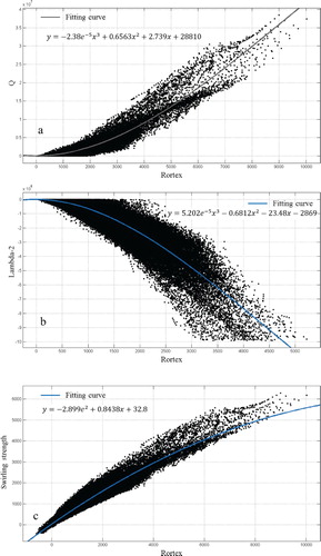
Table 1. Correspondence of the threshold of each method.

Rortex	Q	Lambda-2	Swirling strength
300	88000	−70000	280
550	230000	−210000	490
600	260000	−250000	530
650	300000	−290000	570

By comparing the vortex structures in Figures 6 and 7, it is confirmed that the value of Q criterion, Lambda-2 criterion and swirling strength corresponding to the selected Rortex value determined by the above method is correct. All the four methods have a high similarity in the identification of the global vortex structures, but there are still differences in local areas.

Figure 6. The vortex visualization by Rortex, Q criterion, Lambda-2 criterion and swirling strength at BR = 0.1.

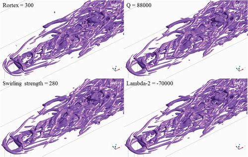
Figure 7. The vortex visualization by Rortex, Q criterion, Lambda-2 criterion and swirling strength at BR = 0.5.

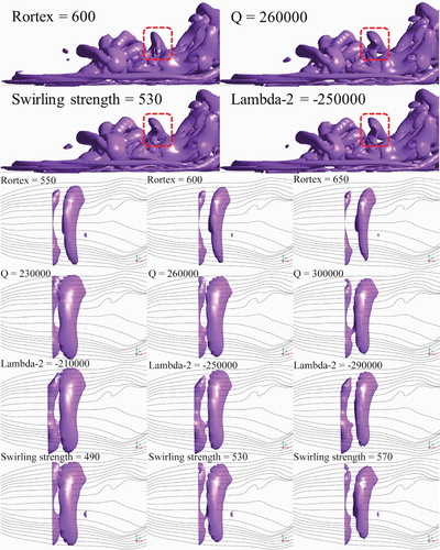
To further illustrate this local difference, Figure 8 shows the vortex group in the evolution region of the downstream at the case BR = 0.5. The overall vortex structures are all basically the same, but there are still some differences, as shown in the red square. Both of Q criterion, Lambda-2 criterion and swirling strength have a zigzag crown vortex structure on the windward side. In contrary, a smooth vortex structure is identified by the Rortex method. In general, there are few zigzag edges in the vortex structure of non-obstacle flow field, because the existence of vortices represents local rotation, and the zigzag edge indicates that the fluid has undergone severe twisting disturbance. And the streamline here is smooth without distortion. This proves that the zigzag vortex structure is unrealistic. Therefore, it is more accurate to use Rortex method than other methods to analyze the characteristics of the vortex structures.

Figure 8. Vortex visualization by Rortex, Q criterion, Lambda-2 criterion and swirling strength with different values and 3D streamlines at BR = 0.5.

4.2. Analysis of vortex evolution

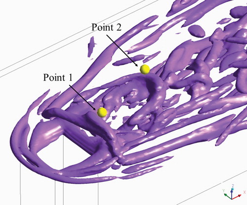
In order to quantitatively study the periodic phenomenon, the measurement points for Rortex value near the jet hole are selected, and the power spectrum density analysis is employed. The dominant vortex structures are generated around the jet hole as shown in Figure 9. Monitoring point 1 is placed at the transmission path of the horseshoe vortex and shear vortex, and monitoring point 2 is placed at the point where the two vortex structures have already merged.

Figure 9. The vortex visualization by Rortex method and the monitoring points at BR = 0.1.

In Figure 10, the shedding process of the horseshoe vortex is shown at BR = 0.1. The horseshoe vortex visualized by Rortex method marked with red line sheds from the wall and can maintain the structural integrity when passing through the jet hole. At T = 15 ms, the horseshoe vortex sheds from the leading side of the hole and the middle of it is raised by the jet flow with its two sides still kept on the wall surface. At T = 17 ms, it is clearly seen that the horseshoe vortex is totally raised up and shed off. However, the hovering vortex generated inside the jet hole keeps close to the inner wall and does not shed off.

Figure 10. The shedding process of horseshoe vortex by Rortex method at BR = 0.1.

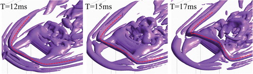
The shedding period of the horseshoe vortex is observed in Figure 11. It can be seen that the horseshoe vortex structures in different times are similar and have obvious periodicity. Therefore, the shedding of the horseshoe vortex is a relatively stable periodic phenomenon. The horseshoe vortex sheds from the wall with a period of approximately 17 ms, therefore the frequency of this periodic phenomenon is estimated to be 1 / 0.017 s = 58.8 Hz.

Figure 11. The horseshoe vortex by Rortex method of the periodic times at BR = 0.1.

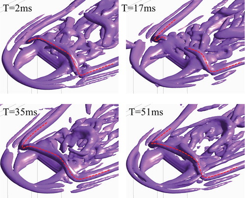
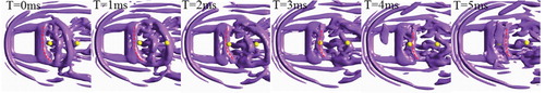
Figure 12 shows the shedding process of the shear vortex by Rortex method at BR = 0.1. The shear vortex is marked with the red line. As shown in the Figure 12, the shear vortex is formed at the rear of the jet hole at T = 0 ms. At first, the middle of it starts to disengage from the jet hole at T = 1 ms. As the shear vortex transports to the downstream region, it is distorted and passing through monitoring point 1 at T = 3 ms. Eventually, the shear vortex sheds from the jet hole at T = 4 ms. Meanwhile, a shed shear vortex is also passing through the monitoring point 2.

Figure 12. The shedding process of shear vortex by Rortex method at BR = 0.1.

In Figure 13, it can be seen that the shedding period of shear vortex is relatively stable, but the shape of the shear vortex is not. There are 4 complete cycles in 0.023 s, so the shedding period of shearing vortex is about 0.0055 s, and the frequency is about 180 Hz.

Figure 13. The shear vortex by Rortex method of the periodic times at BR = 0.1.

The spectrum analysis of Rortex values at point 1 and point 2 are shown in Figure 14. The relative dominate frequency: 60 Hz is corresponding to shedding frequency of the horseshoe vortex and 180 Hz is corresponding to the shedding frequency of the shear vortex in both measuring points. It is worth noting that although the vortex structures corresponding to 60 and 180 Hz are found, there are no corresponding vortex structures whose frequency are 120 and 240 Hz. Because the energy around 120 Hz is so large at point 1, and then it moves to 150 Hz, we speculate that the 120 Hz is the frequency of the entire vortex group. Both of 120, 180 and 240 Hz disperse from point 1 to point 2. In addition, the energy of 240 Hz is small at point 1 but relatively large at point 2, but the frequency is so high that we could not find the corresponding vortex structure in the numerical results. We think it reveals the evolution of a small vortex inside the vortex group.

Figure 14. The power spectrum density of Rortex values at BR = 0.1.

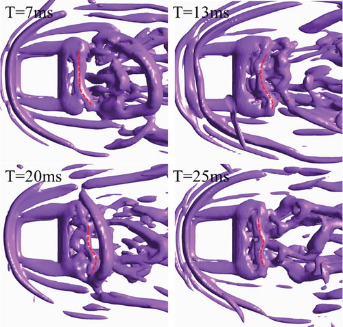
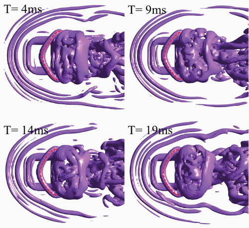
The vortices visualized by Rortex method near the jet hole and monitoring points at BR = 0.5 are shown in Figure 15. In contrast to BR = 0.1, the horseshoe vortex stays at the leading side of the jet hole and does not shed from the wall when BR = 0.5, owing to the strong retard effect of the jet flow. Instead, the hovering vortex generated inside the jet hole sheds off. In Figure 16, the shed process of the hovering vortex marked with the red line is clearly shown. The hovering vortex is formed at the leading side of the jet hole at T = 1 ms. At first, the middle of it starts to disengage from the jet hole and be raised up by the jet flow at T = 2 ms, while its two legs are transported more quickly to the downstream region. As the hovering vortex transported to the downstream region, it is raised up with its two legs linked to the wall and passing through monitoring point 1 at T = 5 ms. Eventually, the hovering vortex mixes with the shear vortex and sheds from the jet hole. In Figure 17, the shapes of the hovering vortex of the periodic times are similar, so the shedding period of the hovering vortex is about 0.005 s (200 Hz).

Figure 15. The vortex visualization by Rortex method and the monitoring points at BR = 0.5.

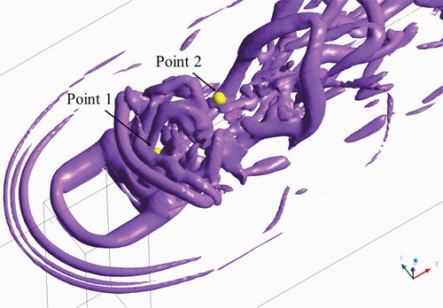
Figure 16. The shedding process of hovering vortex by Rortex method at BR = 0.5.

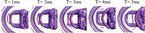
Figure 17. The hovering vortex by Rortex method of the periodic times at BR = 0.5.

However, the shear vortex is strengthened by the shearing effect and the shape of the vortex is not fixed, so it is difficult to identify the generation of vortex from observation.

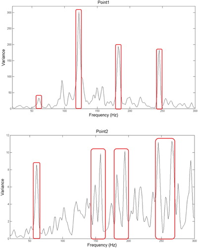
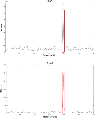
In the spectrum analysis of BR = 0.5 as shown in Figure 18, the dominant frequency is 200 Hz (0.005 s) at both point 1 and point 2, corresponding to the shedding frequency of the hovering vortex. The shapes of them are similar indicating that both the points are affected by the same group of vortex. Compared to the case of BR = 0.1, point 1 and point 2 are completely inside the vortex structures. The power spectrum density of the main frequency is significantly prominent. Therefore, the spectrum analysis can be used to identify the shedding frequency of the dominant vortex structures.

Figure 18. The power spectrum density of Rortex values at BR = 0.5.

5. Conclusion

The jet-in-cross-flow of different values of BR is investigated by using LES, the vortex structures are identified using Rortex, Q criterion, Lambda-2 criterion and swirling strength method. Compared with the four methods, all of them could give similar global vortex structures, while the Rortex method provides more precisely local vortex structures without unrealistic parts.

The spectrum analysis based on Rortex value can effectively identify the shedding frequency of dominant vortex structures in the jet-in-cross-flow process. In the case of two BRs (0.1 and 0.5), the dominant vortex structures has a relatively stable shedding period. When the BR = 0.1, the horseshoe vortex at the leading side of the jet hole sheds off with a shedding frequency of 60 Hz, and the hovering vortex is stable inside the jet hole. The period of the shear vortex is relatively stable, but the shape of the shear vortex varies. When BR = 0.5, due to the enhanced retard effect of the jet flow, the horseshoe vortex is stable in leading side of the jet hole without shedding off, while the hovering vortex is brought out and shedding off with a frequency of 200 Hz owing to the enhancement of the jet flow. The shear vortex is strengthened by the shearing effect and it is hardly observed.

Acknowledgements

The authors would like to acknowledge the financial grants from the national project No. 6140206040301.

Disclosure statement

No potential conflict of interest was reported by the author(s).

Additional information

Funding

This work was supported by National Basic Research Program of China [Grant Number 6140206040301].

References

- Chen, Z. Y., Zhan, J. M., Li, C. W., Hu, W. Q., & Gong, Y. J. (2020). The effect of vortex shedding in film-cooling processes. Heat Transfer Engineering. Advance online publication. https://doi.org/10.1080/01457632.2020.1800260
- Chong, M. S., Perry, A. E., & Cantwell, B. J. (1990). A general classification of three-dimensional flow fields. Physics of Fluids A: Fluid Dynamics, 2(5), 765–777. https://doi.org/10.1063/1.857730
- Coelho, S. L., & Hunt, J. C. R. (1989). The dynamics of the near field of strong jets in crossflows. Journal of Fluid Mechanics, 200, 95–120. https://doi.org/10.1017/S0022112089000583
- Cortelezzi, L., & Karagozian, A. R. (2001). On the formation of the counter-rotating vortex pair in transverse jets. Journal of Fluid Mechanics, 446, 347–374. https://doi.org/10.1017/S0022112001005894
- Demuren, A. O. (1993). Characteristics of three-dimensional turbulent jets in crossflow. International Journal of Engineering Science, 31(6), 899–913. https://doi.org/10.1016/0020-7225(93)90102-Z
- Ekkad, S., & Han, J. C. (2013). A review of hole geometry and coolant density effect on film cooling. Frontiers in Heat and Mass Transfer, 6(1), 1–14. https://doi.org/10.5098/hmt.6.8
- Gao, Y., & Liu, C. (2019). Rortex based velocity gradient tensor decomposition. Physics of Fluids, 31(1), 011704. https://doi.org/10.1063/1.5084739
- Goldstein, R. J. (1971). Film cooling. In T. F. Irvine, & J. P. Hartnett (Eds.), Advances in heat transfer (pp. 321–379). Elsevier.
- Goldstein, R. J., Eckert, E. R. G., & Burggraf, F. (1974). Effects of hole geometry and density on three-dimensional film cooling. International Journal of Heat & Mass Transfer, 17(5), 595–607. https://doi.org/10.1016/0017-9310(74)90007-6
- Gritsch, M., Schulz, A., & Wittig, S. (1998). Adiabatic wall effectiveness measurements of film-cooling holes with expanded exits. Journal of Turbomachinery, 120(3), 549–556. https://doi.org/10.1115/1.2841752
- Grout, R. W., Gruber, A., Yoo, C. S., & Chen, J. H. (2011). Direct numerical simulation of flame stabilization downstream of a transverse fuel jet in cross-flow. Proceedings of the Combustion Institute, 33(1), 1629–1637. https://doi.org/10.1016/j.proci.2010.06.013
- Hasan, N., Sumanta, A., & Srinath, E. (2003). Improved film cooling from cylindrical angled holes with triangular tabs: Effect of tab orientations. International Journal of Heat and Fluid Flow, 24(5), 657–668. https://doi.org/10.1016/S0142-727X(03)00082-1
- Heidmann, J. D., & Ekkad, S. (2008). A novel antivortex turbine film-cooling hole concept. Journal of Turbomachinery, 130, 031020–1. https://doi.org/10.1115/GT2007-27528
- Hunt, J. C., Wray, A. A., & Moin, P. (1988). Eddies, streams, and convergence zones in turbulent flows. (Report No. 89N24555). NASA. https://ntrs.nasa.gov/citations/19890015184
- Islami, S. B., & Jubran, B. A. (2012). The effect of turbulence intensity on film cooling of gas turbine blade from trenched shaped holes. Heat and Mass Transfer, 48(5), 831–840. https://doi.org/10.1007/s00231-011-0938-x
- Islami, S. B., Tabrizi, S. P. A., Jubran, B. A., & Esmaeilzadeh, E. (2010). Influence of trenched shaped holes on turbine blade leading edge film cooling. Heat Transfer Engineering, 31(10), 889–906. https://doi.org/10.1080/01457630903550317
- Jeong, J., & Hussain, F. (1995). On the identification of a vortex. Journal of Fluid Mechanics, 285, 69–94. https://doi.org/10.1017/S0022112095000462
- Kelso, R. M., Lim, T. T., & Perry, A. E. (1996). An experimental study of round jets in cross-flow. Journal of Fluid Mechanics, 306, 111–144. https://doi.org/10.1017/S0022112096001255
- Khajehhasani, S., & Jubran, B. A. (2016). A numerical evaluation of the performance of film cooling from a circular exit shaped hole with sister holes influence. Heat Transfer Engineering, 37(2), 183–197. https://doi.org/10.1080/01457632.2015.1044415
- Kohli, A., & Bogard, D. G. (1997). Adiabatic effectiveness, thermal fields, and velocity fields for film cooling with large angle injection. Journal of Turbomachinery, 119(2), V004T09A044. https://doi.org/10.1115/1.2841118
- Liu, C., Gao, Y., Tian, S., & Dong, X. (2018). Rortex – A new vortex vector definition and vorticity tensor and vector decompositions. Physics of Fluids, 30(3), 035103. https://doi.org/10.1063/1.5023001
- Margason, R. J. (1970). Analysis of the flow field of a jet in a subsonic crosswind. (Report No. 70N21380). NASA.
- Margason, R. J. (1993). Fifty years of jet in cross flow research. In Proceedings of the AGARD Symposium on Computational and Experimental Assessment of Jets in Crossflow, 1, 1-41.
- Mengler, C., Heinrich, C., Sadiki, A., & Janicka, J. (2001). Numerical prediction of momentum and scalar fields in a jet in cross flow: Comparison of LES and second order turbulence closure calculations. In Second Symposium on Turbulence and Shear Flow Phenomena, 2, 425–430.
- Ming Li, H., & Hassan, I. (2015). The effects of counterrotating vortex pair intensity on film-cooling effectiveness. Heat Transfer Engineering, 36(16), 1360–1370. https://doi.org/10.1080/01457632.2015.1003715
- Muppidi, S., & Mahesh, K. (2007). Direct numerical simulation of round turbulent jets in crossflow. Journal of Fluid Mechanics, 574, 59–84. https://doi.org/10.1017/S0022112006004034
- Pietrzyk, J. R., Bogard, D. G., & Crawford, M. E. (1989). Hydrodynamic measurements of jets in crossflow for gas turbine film cooling applications. Journal of Turbomachinery, 111(2), 139–145. https://doi.org/10.1115/1.3262248
- Ruiz, A. M., Lacaze, G., & Oefelein, J. C. (2015). Flow topologies and turbulence scales in a jet-in-cross-flow. Physics of Fluids, 27(4), 045101. https://doi.org/10.1063/1.4915065
- Sun, B. (2019). A new additive decomposition of velocity gradient. Physics of Fluids, 31(6), 061702. https://doi.org/10.1063/1.5100872
- Sykes, R. I., Lewellen, W. S., & Parker, S. F. (1986). On the vorticity dynamics of a turbulent jet in a crossflow. Journal of Fluid Mechanics, 168, 393–413. https://doi.org/10.1017/S0022112086000435
- Tian, S., Gao, Y., Dong, X., & Liu, C. (2018). Definitions of vortex vector and vortex. Journal of Fluid Mechanics, 849, 312–339. https://doi.org/10.1017/jfm.2018.406
- Vaclav, K. (2007). Vortex identification: New requirements and limitations. International Journal of Heat and Fluid Flow, 28(4), 638–652. https://doi.org/10.1016/j.ijheatfluidflow.2007.03.004
- Yuan, L. L., Street, R. L., & Ferziger, J. H. (1999). Large-eddy simulations of a round jet in crossflow. Journal of Fluid Mechanics, 379, 71–104. https://doi.org/10.1017/S0022112098003346
- Yuen, C. H. N., & Martinez-Botas, R. F. (2003). Film cooling characteristics of rows of round holes at various streamwise angles in a crossflow: Part I. Effectiveness. International Journal of Heat & Mass Transfer, 46(2), 237–249. https://doi.org/10.1016/S0017-9310(02)00273-9
- Zhan, J. M., Li, Y. T., Wai, W. H. O., & Hu, W. Q. (2019). Comparison between the Q criterion and Rortex in the application of an in-stream structure. Physics of Fluids, 31(12), 121701. https://doi.org/10.1063/1.5124245
- Zhou, J., Adrian, R. J., Balachandar, S., & Kendall, T. M. (1999). Mechanisms for generating coherent packets of hairpin vortices in channel flow. Journal of Fluid Mechanics, 387, 353–396. https://doi.org/10.1063/1.4933250