Design of a novel vortex-based feedback fluidic oscillator with numerical evaluation

ABSTRACT

In this study, a new vortex-based fluidic oscillator was designed whose performance was numerically evaluated by solving the URANS equations. The oscillator consists of a primary chamber and secondary chamber, separated by a mid-throat and connected by two feedback channels. The jet passing through these chambers forms two pairs of vortices inside the primary and secondary chambers. These vortices roll onto the jet shear layer, and gradually disturbs the jet symmetry. As a result, the vortices grow and shrink asymmetrically, activating the feedback flow to make a harmonic oscillation. The collision of the oscillating jet with the mid-throat traps a part of the jet shear layer in the primary chamber, which forms a strong vortex, returning the jet toward the other side of the mid-throat. The vortex inside the secondary chamber causes the jet to attach to one side of the secondary chamber, deviating the outlet jet to the other side. To compare the performance of the new oscillator with the original one, URANS equations were solved for two-dimensional models of both oscillators with the same grid generation and boundary conditions. The new oscillator had a higher oscillation frequency, a lower pressure drop, and a higher output momentum flux.

KEYWORDS:

• Feedback fluidic oscillator
• vortex-based
• primary and secondary chambers
• numerical
• higher momentum flux

Introduction

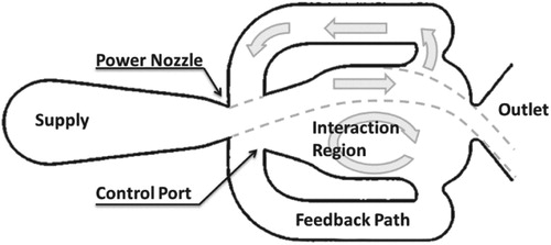
Fluid oscillators have many applications in the field of fluid mechanics and heat transfer, and have been considered by many researchers in fluid mechanics because of their superior properties (Kim & Kim, 2019; Tomac, 2020). Fluidic oscillators do not have any moving parts, and generates weeping jets with various frequencies. The feedback fluidic oscillator, which is shown in Figure 1, is considered as the original fluidic oscillator in this work. It has four parts including: the inlet, outlet, feedback duct, and main diffuser. The Coanda effect causes the jet flow to approach to one of the main diffuser walls, which creates a sweeping jet. Passing fluid through a diffuser causes the fluid to attach to one of the diffuser walls. Hence, the flow is divided into two parts; the first part exits from the outlet, and the second part rebounds to the inlet throat through the feedback duct. Then, the feedback flow collides with inlet flow, which push the inlet flow to the other side of the main diffuser. The repetition of this process forms an oscillating jet.

Figure 1. Fluidic oscillator schematic.

The Strouhal number defines the status of a flow field with instabilities, oscillations, or vortices. The Reynolds (Re) and Strouhal (St) number define the flow field status as follow: (1) $\begin{array}{rl}Re& =\frac{V{D}_h}{\nu }\end{array}$(1) (2) $\begin{array}{rl}St& =\frac{f{D}_h}{v}\end{array}$(2) where V and D_h are the velocity and hydraulic diameter at the inlet throat, v is the kinematic viscosity, and f is the frequency of the oscillations.

Applications

The oscillations of flow in the fluidic oscillators are used in many applications such as heat transfer enhancement of gas turbine blades (Agricola et al., 2018; Hossain et al., 2017; Kim et al., 2017), controlling the flow separation (Andino et al., 2015; Koklu, 2018; Tesař et al., 2013),measuring the mass flow rate (Madadkon et al., 2012) and harvesting energy (Alikhassi et al., 2019).

In some application such as mixing air and natural gas in a dual-fuelled diesel engine (Akbarian et al., 2018), circulation of the irrigant flow inside the root canal to achieve more effective removal of microorganisms (Ghalandari et al., 2019), and making homogenous nanofluids in thermosiphon (Ramezanizadeh et al., 2019), the fluidic oscillators can be effectively used for performance improvement.

In spite of the synthetic jet with temporal oscillations (Xu et al., 2019), the sweeping jet generated by the fluidic oscillator has a spatial oscillation, which can be used for heat transfer enhancement.

Hossain et al. (2018)numerically and experimentally investigated the performance of oscillators in cooling a plate exposed to a hot flow for applications such as gas turbines. The oscillator had a higher heat transfer coefficient than the original methods.

Andino et al. (2015) investigated the performance of oscillators in controlling the separation on the vertical tail of an aircraft. The oscillators significantly increased the suction pressure and increased the lateral force by 20% on the vertical tail.

A 3-D numerical simulation was conducted by Meng et al. (2018) to investigate the enhancement of an axial compressor’s performance and flow control by adding an oscillator. CFX software with the k-ω-SST turbulence model was used to consider variables such as the output jet angle relative to the compressor blades, location, and frequency of the fluidic oscillator.

Kara (2017) numerically investigated the effect of adding an oscillator to a hump-shaped geometry and reducing the separation bubble by two-dimensional unsteady Reynolds-averaged Navier-Stokes (URANS) equations with the k-ω SST turbulence model.

Madadkon et al. (2012) used a fluidic oscillator to measure the water mass flow rate in a pipeline in a Reynolds number range of 300–50000. The characteristic diagram of the flow meter was obtained by the measurement of static pressure fluctuations.

Alikhassi et al. (2019) used a fluidic oscillator to effectively convert the kinetic energy of a fluid into the strain energy of a piezoelectric structure. The relationship between the input velocity and the frequency of fluid fluctuations in the fluidic oscillator was obtained, and different positions were examined for the piezoelectric beam and the effect of the input velocity on the output voltage.

Performance parameters of the original oscillator

Many numerical and experimental studies have been carried out to study the flow pattern inside or outside a fluidic oscillator. Seo and Mittal (2017) numerically studied the fluid flow inside a fluidic oscillator by using the second-order finite element Navier-Stokes equations and applying the Crank–Nicholson scheme for time derivative terms. They concluded that a separation bubble is formed near the wall, which is the main reason of fluctuations. They also showed that an increase in the length of the feedback duct decreases the amplitude and harmony of the oscillations. The oscillation frequency did not change much by changing the length of the feedback channel while an increase in the length of the oscillator decreased the frequency.

Vasta et al. (2012) used the k-ϵ model in a numerical investigation of a fluidic oscillator, which was very similar to the original oscillator. They found that the numerical results for mean and standard deviations of jet velocity profile agreed well with experimental data.

Krüger et al. (2013) numerically studied the flow inside a fluidic oscillator with sharp corners and compared the numerical results with PIV and time-resolved pressure measurements. They used unsteady Reynolds-averaged Navier-Stokes equations (URANS) with k-ω SST turbulence model. The 2Dnumerical solution with the SST turbulence model was sufficient to qualitatively and quantitatively describe the flow field.

Pandey and Kim (2018) used large eddy simulation (LES) and Unsteady Reynolds-averaged Navier-Stokes (URANS) analysis to study the flow of a feedback fluidic oscillator with sharp corners. The k-ω SST model was used for turbulence closure in the URANS analysis, and the WALE model was used for the large eddy simulation. The numerical results were qualitatively and quantitatively compared to the available experimental results of the flow field and frequency of the jet oscillation to verify the numerical solution. The RANS analysis showed better overall agreement with the experimental data than the large eddy simulation. The URANS analysis correctly predicted the vortical structures in the feedback channels and mixing chamber.

Jeong and Kim (2018) optimized the shape of a fluidic oscillator by a 3D transient numerical study via CFX software. The standard k-ϵ, k-ω SST, and BSL turbulence models were used and compared with experimental data. For the k-ϵ model, good agreement was obtained between the numerical and experimental results of the frequencies. For optimization, two variables were considered: the ratio of the width of the inlet nozzle to the outlet width and the ratio of the width of the splitter to the outlet nozzle width. The objective functions were defined to achieve the maximum velocity of output jet and minimum pressure drop of the oscillator.

B. C. Bobusch et al. (2013) investigated the effect of the length and volume of the feedback channel, the inlet area to the main chamber, nozzle width, outlet jet displacement angle, and pressure drop on the oscillation frequency. They carried out a 2D transient numerical solution with the k-ω SST turbulence model using CFX software. They validated their numerical results with flow pattern data from particle image velocimetry (PIV) experiments. The results showed that the oscillation frequency and angle of the output jet are independent of the walls of the diverging nozzle.

Ostermann et al. (2015) investigated the flow pattern inside and outside two different oscillators with curved walls and sharp edges by PIV technique. They concluded that the oscillation frequencies of both oscillators varied linearly with the mass flow rate. However, for the curved oscillator, flow separation in the feedback channels’ corners was reduced. Then, the curved oscillator was optimized based on the mean pressure drop. They showed that the inlet pressure needed to be about 20% lower to create a uniform discharge.

Mohammadshahi et al. (2020) experimentally studied the flow pattern outside a fluidic oscillator and investigated the effect of the external domain on the oscillation frequency and maximum deflection angle. They concluded that the external domain does not have a significant effect on the frequency. However, the flow pattern was completely dependent on the external domain.

Woszidlo et al. (2015) experimentally studied the flow characteristics of an oscillator inside and outside an oscillator via PIV measurement. They concluded that by increasing the flow rate, the frequency of the oscillating pattern increases almost linearly. However, increasing the inlet velocity leaded to an increase in the flow rate from the feedback channels. The total volume of this fluid normalized by the oscillation frequency was constant over a period of the oscillation and was equal to the volume needed to enlarge the separation bubble. The results showed that the frequency of the oscillations depended on the volume required to grow the separation bubble and the essential time to transfer the fluid volume.

The basis of the original oscillator is the Coanda effect which causes the jet to completely attach to the wall in a short time, and detach from the wall by a high flow rate of the feedback channel. The large space inside the original oscillator causes the amplitude of jet oscillation inside the oscillator to be very high. These factors depreciate the jet momentum and causes a high pressure loss inside the original oscillator. In this research, a novel fluidic oscillator was designed to decrease the space and oscillation amplitude inside the oscillator, and to decrease the flow rate through the feedback channel. The jet inside the new oscillator has a minimum attachment with the walls so that the Coanda does not almost affect the flow behavior. The performance was evaluated by a 2D numerical solution of URANS equations with the k-ϵ RNG turbulence model. The mechanism of the oscillator is based on two pairs of vortices inside the primary and secondary chambers, which roll onto the jet shear layer. The main reasons for instability and oscillation inside the new oscillator are the interaction of four vortices with the fluid jet and their instability when they grow and shrink.

Geometry definition and design considerations

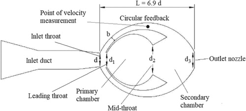
The new oscillator shown in Figure 2 consists of a primary chamber and a secondary chamber, which are separated by a mid-throat and connected by two circular feedback channels. The idea of the new geometry was obtained from a duct with wavy walls, which cause some vortices to be formed between the jet flow and the wavy walls. Without feedback channels, the jet flow will be symmetric, and there will be no oscillation in the flow. Adding the feedback channels and choosing the appropriate values for the design parameters cause the vortices to grow and shrink asymmetrically, and form the oscillations. The dimensions are specified in Figure 2. The important design considerations of the new oscillator are as follow:

• The throat at the trailing edge of the feedback channel should be approximately 10% more than the inlet throat (1.1 d). This distance should be set in a way that the shear layer of the inlet jet is approximately tangent to the trailing edge of the feedback channel. This makes it hard for the flow through the feedback channel to enter the primary chamber, and the flow rate of the feedback channel decreases. However, after oscillation, the flow through the feedback channel will be increased. If the throat at the trailing edge of the feedback channel is much larger than 1.1 d, the pressure difference between the secondary and primary chambers will be equal, and no oscillation will occur (See Figures 23a and 24a). On the other hand, if this throat is less than the inlet throat (d), the leading edge interacts with the jet core, which disrupts the jet.

• The nozzle outlet throat was selected to be slightly smaller than the width of the fluid jet before beginning the oscillation. This means that the shear layer of the jet at the outlet section should slightly collide with the outlet throat. If the outlet throat is wider than the fluid jet width before beginning the oscillation, the pressure inside and outside of the chamber will be the same, and no oscillation will occur (see Figures 8c, 23c, and 24c).

• The mid-throat should be wider than the jet width. The shear layer of the jet should not collide with the mid-throat before starting the oscillation. The mid-throat limits the oscillation amplitude. The larger the middle throat, the greater the amplitude of jet oscillation will be. On the other hand, if the mid-throat is much wider than the jet width, the interaction of the jet with the mid-throat decreases, and the jet cannot form intense vortices inside the primary chamber at the initial time, which are very important for starting the jet oscillation (see Figures 8c, 23b, and 24b).

• The design of the feedback channel was based on considering a channel between the primary and secondary chambers with a minimum curvature. The trailing edge of the feedback channel should be approximately tangent to the shear layer of the inlet jet as explained above. The width of the feedback channel was chosen to be less than that of the original oscillator shown in Figure 1. This causes the flow rate through the feedback channel to decrease relative to the original, which reduces the momentum depreciation of the jet and increases the fluidic oscillator's efficiency. However, a large reduction of the feedback channel width will cause the oscillation to stop (See Figures 23d and  24d).

• The angle of the secondary chamber wall after the mid-throat was obtained by observing the flow field and matching the fluid jet angle to the wall at maximum jet deflection.

• The angle at the end of the secondary chamber wall has a direct effect on the outlet jet angle. The angle has been set in a way that the outlet jet angle of the new oscillator is approximately equal to that of the original oscillator.

Figure 2. The dimensions of the new fluidic oscillator design.

Governing equations

To analyze the flow oscillations inside and outside the fluidic oscillator, the finite volume method was used to solve the two-dimensional unsteady Reynolds-averaged Navier-Stokes (URANS) equations, which describe the conservation of the mass and momentum as follow: (3) $\begin{array}{rl}& \frac{\mathrm{\partial }\overline{u_i}}{\mathrm{\partial }{x}_i}=0\end{array}$(3) (4) $\begin{array}{rl}& \frac{\mathrm{\partial }\overline{u_i}}{\mathrm{\partial }t}+\overline{u_j}\frac{\mathrm{\partial }\overline{u_i}}{\mathrm{\partial }{x}_j}=-\frac{1}{\rho }\frac{\mathrm{\partial }p}{\mathrm{\partial }{x}_i}+\vartheta \frac{\mathrm{\partial }}{\mathrm{\partial }{x}_j}\left(\frac{\mathrm{\partial }\overline{u_i}}{\mathrm{\partial }{x}_j}+\frac{\mathrm{\partial }\overline{u_j}}{\mathrm{\partial }{x}_i}\right)\\ & -\frac{\mathrm{\partial }}{\mathrm{\partial }{x}_j}\left(\overline{u_i^{\mathrm{\prime }}{u}_j^{\mathrm{\prime }}}\right)\end{array}$(4)

In spite of many advantages of RANS predictions for turbulent flows, RANS equation only describes flows in a statistical scheme to use time-averaged pressure and velocity fields. This approach cannot distinguish quasi-periodic large-scale and turbulent chaotic small-scale structures of the flow field. This causes some problems, especially when both phenomena are present in the flow field (Breuer et al., 2003). On the other hand, LES operates with unsteady fields of physical values. The principal idea behind LES is to reduce the computational cost by ignoring the smallest length scales, which are the most computationally expensive to resolve, via spatial filtering of the Navier–Stokes equations instead of averaging in time (Breuer et al., 2003). However, the large-scale vortical structures have the main role in describing the flow inside the fluidic oscillator. Because, the differences between RANS and LES are mainly related to the detailed flow field, and LES cannot be used for two-dimensional flow and has a high computational cost, the URANS analysis was chosen for the current flow analysis.

Numerical scheme and turbulence model

A second-order implicit time integration scheme was used for the transient formulation. The pressure correction and momentum equations were coupled. The PISO algorithm combined the continuity and momentum equations to derive the pressure correction equation. The variables were interpolated from the cells’ centers to their faces by a quick discretization. The Reynolds stress terms in the momentum transport equations were resolved using the k-ϵ RNG turbulence model. The k and ϵ at the inlet were calculated based on the turbulence intensity of 5% and the hydraulic diameter of 0.03 m. A zero gradient of k and ϵ was considered at the outlet.30 iterations at each time step were considered to ensure the convergence at each time step.

The k-ϵ RNG turbulence model rely on the Boussinesq hypothesis, which links the Reynolds stress tensor with the mean deformation rate tensor to reduce the computational cost of the determination of the turbulent viscosity. The main disadvantage of this hypothesis is that it assumes that the turbulence is isotropic.

The $k-\epsilon$ model ignores the small-scale structures, and replaces them with large-scale structures. It can effectively be used for industrial applications because of its good convergence rate and low computational cost. In addition, the $k-\epsilon$ is appropriate for the external flow overcomplicated bodies. However, the $k-\epsilon$ is not suitable for the flows with adverse pressure gradients or jet flow, and over-predicts the shear-stress and turbulent length-scale in the near wall region or jet shear layer. The $k-\epsilon$ model calculates the eddy viscosity from a single turbulence length scale. Thus, the turbulent diffusion is calculated only based on the specified scale, another scales of motion are not considered in the turbulent diffusion.

Yakhot et al. (1992) developed the RNG model to renormalize the Navier-Stokes equations, and to consider the effects of small-scales structures. The RNG model derives a turbulence model (Equations (6) and (7)) with a modified form of the epsilon equation (Equation (7)). A differential formula for the effective viscosity, an analytical formula for turbulent Prandtl number, and the effect of swirl in turbulence are considered in the RNG model. These benefits improves the prediction for (a) high-curvature streamlines and high strain rate, (b) transitional flows, and (c) heat and mass transfer near the wall. However, this model has a high computational overhead. (5) $\begin{array}{rl}& -\rho \overline{u_i^{\mathrm{\prime }}{u}_j^{\mathrm{\prime }}}={\mu }_t\left(\frac{\mathrm{\partial }{u}_i}{\mathrm{\partial }{x}_j}+\frac{\mathrm{\partial }{u}_j}{\mathrm{\partial }{x}_i}\right)-\frac{2}{3}\left(\rho k+{\mu }_t\frac{\delta u_i}{\delta x_i}\right){\delta }_{ij}\end{array}$(5) (6) $\begin{array}{rl}& \frac{\mathrm{\partial }}{\mathrm{\partial }t}\left(\rho k\right)+\frac{\mathrm{\partial }}{\mathrm{\partial }{x}_j}\left(\rho k{u}_j\right)\\ & =\frac{\mathrm{\partial }}{\mathrm{\partial }{x}_j}\left[\left[\left(\mu +\frac{{\mu }_t}{{\sigma }_k}\right)\frac{\mathrm{\partial }k}{\mathrm{\partial }{x}_j}\right]\right]+{\mu }_t{S}^2-\rho ϵ\end{array}$(6) (7) $\begin{array}{rl}& \frac{\mathrm{\partial }}{\mathrm{\partial }t}\left(\rho \epsilon \right)+\frac{\mathrm{\partial }}{\mathrm{\partial }{x}_j}\left(\rho \epsilon u_j\right)=\frac{\mathrm{\partial }}{\mathrm{\partial }{x}_j}\left[\left[\left(\mu +\frac{{\mu }_t}{{\sigma }_k}\right)\frac{\mathrm{\partial }\epsilon }{\mathrm{\partial }{x}_j}\right]\right]\\ & +C_{1\epsilon }\frac{\epsilon }{k}{\mu }_t{S}^2-C_{2ϵ}^{\ast }\rho \frac{{ϵ}^2}{k}\end{array}$(7) (8) $\begin{array}{rl}& C_{2ϵ}^{\ast }=C_{2\epsilon }+\frac{C_{\mu }{\eta }^3\left(1-\eta /{\eta }_0\right)}{1+\text{β}{\eta }^3},{\mu }_t=\rho C_{\mu }\frac{k^2}{\epsilon },\\ & \eta =\frac{Sk}{\epsilon }\text{ and }S=(2S_{ij}{S}_{ij}{)}^{1/2}\end{array}$(8)

Table

$C_{\mu }$	${\sigma }_k$	${\sigma }_{\epsilon }$	$C_{1\epsilon }$	$C_{2\epsilon }$	${\eta }_0$	β
0.0845	0.7194	0.7194	1.42	1.68	4.38	0.012

Validation

A common fluidic oscillator with sharp corners was considered for the validation of the current flow solver because the new oscillator has some sharp edges too. The flow inside the common fluidic oscillator with sharp corners was numerically solved, and its results were compared to the numerical and PIV results of Krüger et al. (2013). The geometry and solution conditions were considered the same as that used in Krüger et al. (2013), as shown in Table 1. Figure 3 qualitatively compares the axial velocity field at a specified time (t = 0.65 T) for the current study and Krüger’ study. In addition, Figure 4 compares the quantitative axial velocity distribution along the line shown in Figure 3(c). As it can be seen, there is good agreement between the current results and Krüger’s results. Figure 5 plots the velocity fluctuations versus time at a point shown in Figure 3(c). The oscillations frequency can be obtained by a Fast Fourier Transform (FFT) of the velocity fluctuations (Figure 5). Table 2 also shows a good agreement between the oscillations frequency of the common oscillator with sharp corners, which were obtained by the current numerical solution, and the PIV and numerical solution in Krüger et al. (2013).

Figure 3. Comparison of instantaneous axial velocity field at t = 0.65 T between 2D SST numerical results of the current study, and the PIV results and 2D SST numerical results of Krüger et al. (2013).

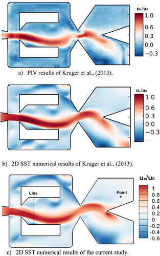
Figure 4. Quantitative comparison of axial velocity distribution along the line shown in Figure 3(c).

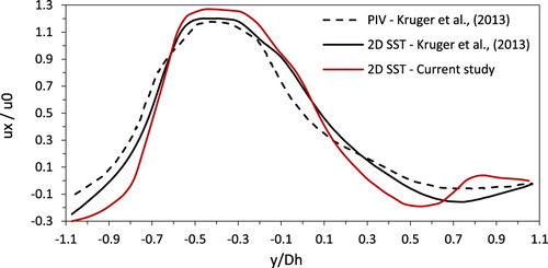
Figure 5. Velocity fluctuation at the point shown in Figure 3(c) versus flow time and FFT diagram for the oscillator with sharp edges.

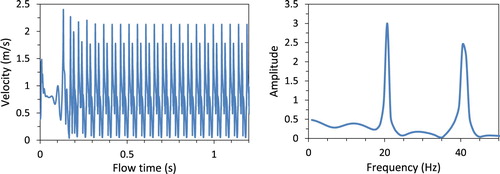
Table 1. Overview of solution conditions for the current study and Krüger et al. (2013).

	Numerical solution of Krüger et al. (2013)	Current numerical solution
Turbulence model	k-ω SST	k-ω SST
Inlet velocity (m/s)	1.2	1.2
Inlet throat velocity (m/s)	3.9	3.9
Kinematic viscosity (m2/s)	1.004×10^−6	1.004×10^−6
Reynolds number	16,034	16,027
Grid type	Structured	Structured
Grid elements	135,153	120,806
Maximum Y^+	–	5

Table 2. Oscillations frequency for the current study and Krüger et al. (2013).

	2D SST- current study	2D SST-Krüger et al. (2013)	PIV-Krüger et al. (2013)
Frequency (Hz)	20.7	20.9	21.5

Grid generation and boundary conditions

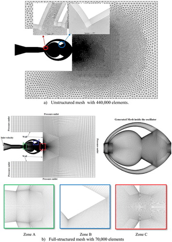
The first and most important step of the numerical simulation of the flow inside the new fluidic oscillator is the grid generation. In this simulation, semi-structured and unstructured grids were used near the walls and away from the walls, respectively (Figure 6a). A full-structured mesh (Figure 6b) was also used for the whole domain inside and outside the oscillator to check the effect of mesh type on the solution. Almost uniform fine grids were used inside the whole oscillator because the flow is completely oscillatory with many harmonic vortices and recirculating flow. A large space outside the oscillator was considered for flow to reach the ambient pressure smoothly. The working fluid was water, and the boundary conditions were considered the velocity at the nozzle inlet and ambient pressure at the outlet. Figure 6 shows the computational domain and grids for inside and outside the fluidic oscillator. The ambient pressure was set far from the nozzle outlet to let the sweeping jet smoothly reach the ambient pressure. For initialization, Laplace's equation was solved initially to determine the velocity and pressure fields as initial guess.

Figure 6. The grid and computational domain for numerical flow solution.

Grid and time step independence study

The frequency of the flow oscillation inside the feedback channel was considered as the parameter to evaluate four grid configurations (Figure 7a) and to determine the influence of mesh size on the solution. In Figure 7(a), it is observed how the oscillation frequency reaches an asymptotic value as the number of elements increases. According to this figure, both meshes with 70,000 and 440,000 elements were considered to be sufficiently reliable to ensure mesh independency. The averagedY⁺ near the walls was less than 4 for all wall surfaces for these meshes. Table 3 show the averaged Y⁺ for each mesh. Figure 4(b) compares the FFT diagrams for two meshes with 28,000 and 70,000 elements. As can be seen, some irregular fluctuations for the grid with 28,000 elements are removed by increasing the number of elements. Because the FFT for the finest grid is the same as that for the grid with 70,000 elements, only these two grids were compared.

Figure 7. Effect of grid size on the oscillation frequency.

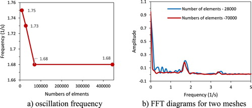
Table 3. Averaged Y+ for each grid.

Number of elements	Grid 1 (9,000)	Grid 2 (28,000)	Grid 3 (70,000)	Grid 4 (440,000)
Averaged Y^+	20	12	8.5	4

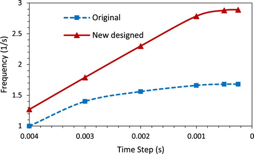
The effect of the time step on the frequency of both the oscillators was also studied, as shown in Figure 8. The time step of 0.0005s for the unstructured mesh and 0.00005sfor the full-structured mesh were small enough to correctly capture the oscillation frequency.

Figure 8. Effect of time step on the oscillation frequency.

To perform an additional verification of the current numerical analysis, the frequency of the original feedback fluidic oscillator (Figure 1) was compared with that of an experiment. To calculate the frequency from the numerical solution, a point in the feedback channel was considered to plot the velocity versus time. Figure 9 shows an example of velocity fluctuations in the feedback channel of each oscillator at Re = 60000. The Reynolds number of the new oscillator was defined based on the jet velocity and hydraulic diameter at the inlet throat similar to Equation (1), which was defined for the original feedback fluidic oscillator. Comparison of velocity fluctuations in the feedback channel shows that the fluctuations of the new oscillator are more harmonic than that of the original one. The oscillations frequency can be obtained by a Fast Fourier Transform (FFT) of the velocity fluctuations for both oscillators. Figure 9 also compares the FFT diagrams of the velocity fluctuations for both oscillators.

Figure 9. Velocity of flow through the feedback channel versus flow time and FFT diagram for the two oscillators at Re = 60,000.

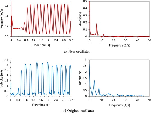
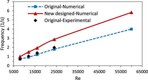
Figure 10 shows how the frequency linearly changes with the Reynolds number for both the oscillators. The new oscillator has a higher frequency than the original one. The numerical frequency of the original oscillator was compared with that of the experiment (Kim et al., 2017) which shows a good agreement. In addition, a qualitative comparison between the instantaneous velocity contours inside the original oscillator, which were obtained from the current numerical solution (See Figure 16) and the PIV results of Ostermann et al. (2015), shows a good agreement.

Figure 10. Comparison of the frequency versus Re for the two oscillators.

Results and discussion

Initial phases of forming the jet in the new oscillator

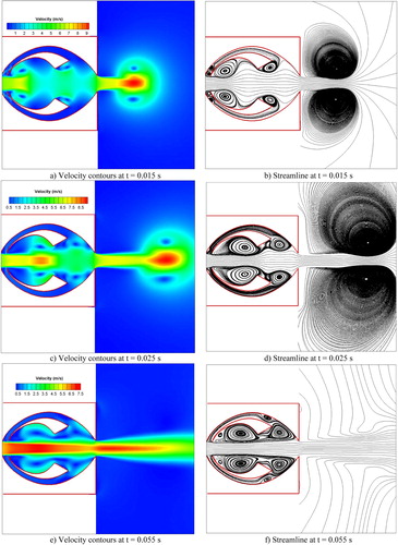
This part explains how the flow field forms inside and outside the new oscillator at initial time steps. Figure 11 shows how two pairs of vortices are formed and grow in the primary and secondary chamber, when the fluid jet enters the oscillator. According to this figure, two pairs of vortices are formed in the early moments of the flow passing through the primary and mid-throats (Figure 11a and b). The formation of a continuous jet inside the chamber intensifies the vortices (Figure 11e and f), and then they start to roll over the shear layer of the jet. This causes the symmetry of the jet above and below the shear layer to be destroyed. By destroying the symmetry of the jet, the upper and lower vortices asymmetrically grow and shrink, which causes the amplitude of the oscillations to increase gradually, and the oscillation amplitude reaches the maximum value.

Figure 11. Contours of velocity and streamlines at the initial times at Re = 60,000.

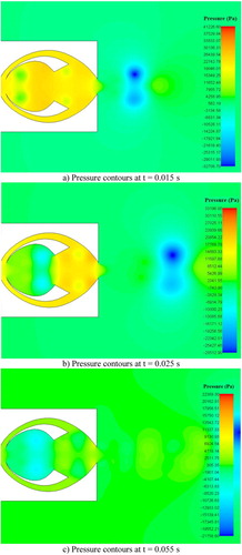
The pressure contours in Figure 12 show how the strong vortices inside the primary chamber reduce the pressure inside the primary chamber due to their high vorticity. As can be seen, the pressure inside the primary chamber decreases with the time, which shows that the vortices inside the primary chamber are intensifying. Since the outlet nozzle throat is smaller than the mid-throat, the pressure inside the secondary chamber increases. The pressure difference between the primary and secondary chambers gradually activates the feedback channels.

Figure 12. Contours of pressure at the initial times at Re = 60,000.

Comparison between the new and original oscillator

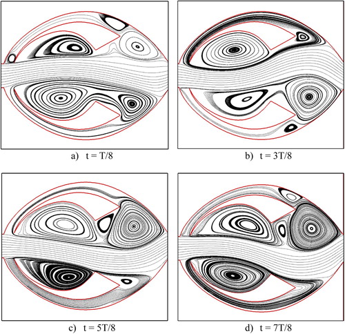
The performances of the new and original oscillator after reaching harmonic oscillations are compared in this section. Figure 13 shows how the two pairs of vortices asymmetrically grow and shrink at different steps of a time period, which form a sinusoidal shape for the jet inside the oscillator. According to this figure, the jet inside the new oscillator mainly collides with the two pairs of vortices instead of colliding with the wall. It can cause less depreciation of the jet momentum and lower pressure loss inside the new oscillator.

Figure 13. Streamlines inside the oscillator at 4 equal intervals of a time period after forming the harmonic oscillations at Re = 60,000.

Figures 14 and 15 respectively show the velocity and pressure contours of the new oscillator at eight equal intervals of a time period at Re = 60000. The jet fluctuates well through the new oscillator. As mentioned, the onset of the oscillations is caused by destroying the symmetry of the two pairs of vortices inside the chambers. Asymmetrical growth and shrinkage of these two pairs of vortices increase the jet oscillation. The maximum amplitude of the jet oscillations inside the oscillator is constrained by the mid-throat. If the mid-throat is larger than a specified value, the oscillator will not work well (See Figures 26b and 27b) because the vortices in the primary chamber will be so weak that they cannot disturb the asymmetry of the jet.

Figure 14. Contours of velocity at 8 equal intervals of a time period in the new designed oscillator at Re = 60,000.

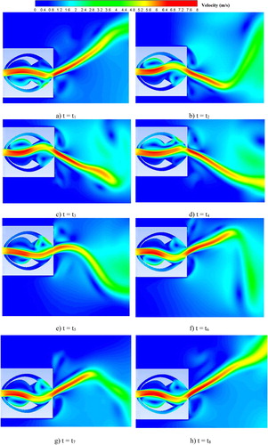
Figure 15. Contours of pressure at 8 equal intervals of a time period in the new designed oscillator at Re = 60,000.

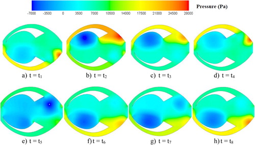
During the jet oscillation, as the jet approaches the upper wall of the middle chamber (Figure 14), a part of the shear layer is trapped inside the upper part of the primary chamber, and intensifies the vortex (Figure 14b), which decreases the pressure inside the trapped vortex (Figure 15b). Within a short time, the intensified vortex returns the jet downward (Figure 14c and d), which decreases the pressure and intensity of the trapped vortex (Figure 15c and d). As the jet approaches the upper wall of the mid-throat, the second half of the jet inside the oscillator attaches to the upper wall of the secondary chamber, which shrinks the vortex near the upper wall of the secondary chamber and pushes the trapped fluid into the upper feedback channel (Figure 14b). Due to the collision of the jet with the upper end wall of the secondary chamber, the pressure increases in this region (red-coloured region in Figure 15b).

This increases the pressure inside the upper feedback channel and pushes the jet downward, which opens the gap between the jet and the trailing edge of the feedback channel to let the feedback flow enter the primary chamber (Figures 14b and 15b). Therefore, the upper feedback flow feeds the shear layer of the jet core, which intensifies the trapped vortex in the upper side of the primary chamber (Figure 14b). The intensified trapped vortex quickly returns the jet from the upper wall of the mid-throat (Figures 14c and 11d). When the jet is attached to the upper wall of the secondary chamber, the exiting jet outside the oscillators deflected downward (Figure 14b and c).

As the jet inside the oscillator deflects downward, the upper feedback channel at the conjunction with the inlet jet opens more, and the flow of upper feedback is easily permitted to enter into the upper part of the primary chamber to feed the intensified vortex in this region (Figure 14c and d). While the fluid jet moves away from the upper wall of the mid-throat, the vortex formed inside the upper part of the primary chamber is permitted to fill both the upper part of the primary and secondary chamber (Figure 14d), which causes the difference between the pressure of the upper parts of the primary and secondary chambers to decrease (Figure 15d). After a while, this vortex is divided into two vortices above the jet in the primary and secondary chambers (Figure 14e).

When the jets are moving downward, the movement of the first half of the jet is limited by the vortex trapped inside the lower side of the primary chamber and by the mid-throat. The second half of the jet freely moves downward to reach the lower wall of the secondary chamber (Figure 14e and f). At this time, the trapped vortex above the second half of the jet intensifies, which decreases the pressure in this region (Figure 15e). This intensified vortex in the secondary chamber attaches the jet to the lower wall of the secondary chamber (Figure 14g). This process repeats over and over again. A similar process occurs in lower Reynolds numbers.

The flow fields of the original oscillator were compared to those of the new oscillator using two-dimensional numerical simulations with the same numerical method, boundary conditions, and grid generation. Figure 16 shows the velocity field at the same eight equal intervals of a time period. The upper and lower bounds of the contours are exactly the same as in Figures 14 and 16. The contours also have the same scale and are comparable in size. One of the benefits of the new oscillator is its smaller size than the original geometry, which reduces the jet energy loss and jet discontinuity along the path and increases the frequency of oscillations. In addition, the jet inside the new oscillator collides with the two pairs of vortices instead of colliding with the wall. It causes less depreciation of the jet momentum and lower pressure loss inside the new oscillator.

Figure 16. Contours of velocity at 8 equal intervals of a time period in the original oscillator at Re = 60,000.

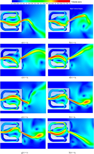
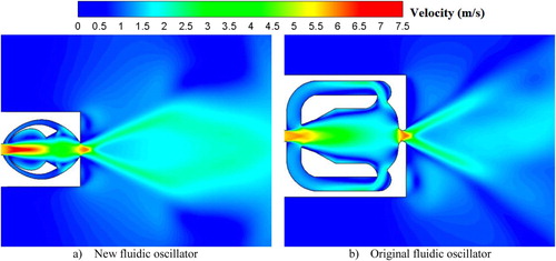
Comparison of the fluid jet outside the oscillators indicates that the jet velocity far from the outlet is higher for the new oscillator. It indicates that the jet outside the new oscillator has a longer persistence when getting away from the outlet. Due to the smaller diameter of the outlet nozzle in the original oscillator, a higher velocity can be seen in some places near the outlet nozzle of the original oscillator (Figure 16b). However, high momentum loss is quite evident as the jet moves away from the outlet nozzle in the original oscillator. The qualitative comparison shows that the output jet angle in the two oscillators is approximately equal. A qualitative comparison between the instantaneous velocity contours inside the original oscillator (Figure 16) and the PIV results of Ostermann et al. (2015) shows a good agreement.

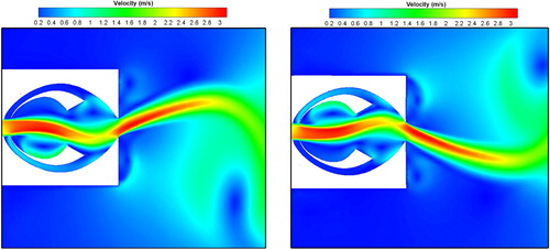
To compare the flow fields of the two oscillators, the time-averaged velocity field in several time periods is shown in Figure 17. The power of the fluid jet in the new oscillator has been significantly increased. Figure 17(a) clearly shows the two pairs of vortices, even in the time-averaged velocity contour. The flow rate through the feedback channel of the new oscillator is less than that of the original one. The ratio of the feedback channel discharge to the input discharge for the new designed oscillator is one-fifth of that for the original oscillator, which causesless depreciation of the jet momentum and lower pressure loss inside the new oscillator.

Figure 17. Comparison of time-averaged velocity contours for the two oscillators at Re = 60,000.

One of the design considerations of this oscillator was the reduction of the flow rate through the feedback channel, which reduces the momentum depreciation of the fluid jet and increases its efficiency. This goal was achieved by reducing the width of the feedback channel and the distance of its trailing edge from the jet shear layer at the entrance to the primary chamber. In this design, the primary chamber plays a key role in the fluid jet deflection, and the feedback channel plays an auxiliary role. However, the absence of a feedback channel stabilizes the fluid jet and prevents the oscillation.

To compare the velocity profile outside the nozzle outlet, Figure 18(a) shows the time-averaged velocity vector plot along 11 sections perpendicular to the oscillator axis. For a better comparison, Figure 18(b) plots the axial velocity distributions along three vertical sections with equal distance from the outlet nozzles for the two oscillators. Except in the region near the outlet nozzle, the new oscillator has a higher jet velocity.

Figure 18. Comparison of the time-averaged vector plot and velocity distributions of the original and new oscillators at different sections outside the outlet nozzle at Re = 60,000.

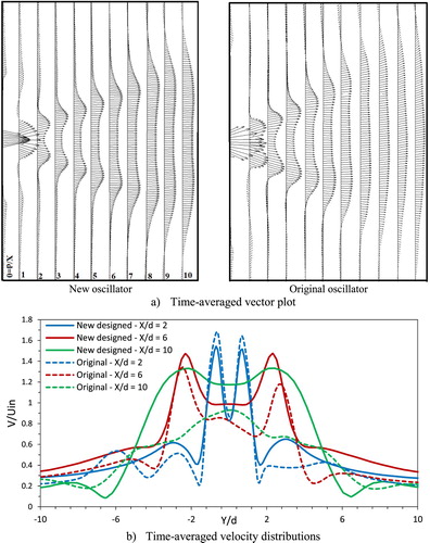
Figure 19 compares the distribution of the non-dimensional mass and momentum flux versus axial distance for the two oscillators. The mass and momentum fluxes were calculated at each section according to Equations (9) and (10), and then nondimensionalized by the mass and momentum fluxes at the inlet throat. (9) $\begin{array}{rl}\dot{m}& ={\int }_{-H/2}^{H/2}\rho udy\end{array}$(9) (10) $\begin{array}{rl}M& ={\int }_{-H/2}^{H/2}\rho u^{2}dy\end{array}$(10) where H is the height of the domain outside the oscillator and u is the axial velocity. The momentum fluxes were calculated from the numerical time-averaged velocity vector plot along the same sections shown in Figure 18(a).

Figure 19. Comparison of the non-dimensional mass and momentum flux of the original and new oscillators at 10 sections outside the outlet nozzle at Re = 60,000.

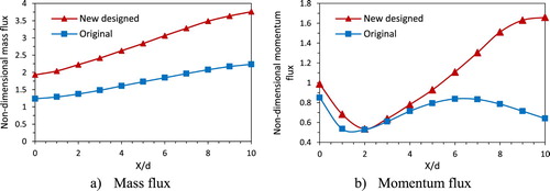
Figure 19 shows that both mass and momentum fluxes outside the new oscillator are higher than those outside the original oscillator. It means that the jet outside the new oscillator sucks the surrounding fluid toward the jet more than the original oscillator. The difference between the momentum fluxes of the two oscillator increases along the axial distance. For X/d > 5, the momentum flux of the new oscillator significantly increases compared to that of the original oscillator. The momentum flux at X/d = 10 is 60% higher than that at X/d = 0 for the new oscillator while at all sections, it is less than that at X/d = 0 for the original oscillator.

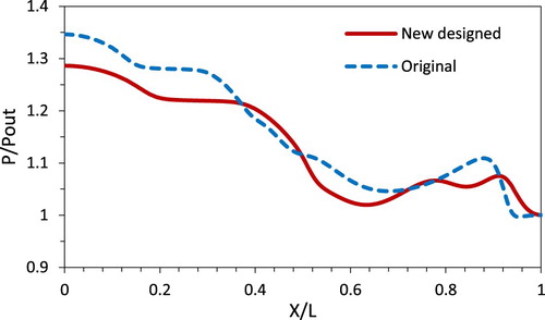
In Figure 20, the time-averaged pressure contours are compared for the two oscillators. According to the pressure contours of the new oscillator, the pressure inside the primary chamber decreases to ambient pressure, and then increases again inside the secondary chamber. The decrease of pressure in the primary chamber is due to the pressure reduction inside the vortex core formed in this chamber. The decrease of pressure in the primary chamber sucks the feedback flow into the primary chamber. The pressure difference between the primary and secondary chambers plays an important role in the instability and oscillation of the jet. Specifically, at the initial times, the strength of the vortices formed in the primary chamber is very high, resulting in a lower pressure in the primary chamber (See Figure 12b and c), which is an important factor for the jet oscillation. Figure 20 also shows a lower pressure drop through the new oscillator compared to the original oscillator. Figure 21 compares the pressure ratio distributions along the center line of both oscillators versus the non-dimensional axial distance from the inlet to the outlet nozzle. As seen, the ratio of inlet to outlet pressure in the new oscillator is 5% less than that in the original one.

Figure 20. Comparison of time-averaged pressure contours for the two oscillators at Re = 60,000.

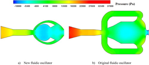
Figure 21. Comparison of pressure ratio distribution along the axis of the two oscillators at Re = 60,000.

Effect of Reynolds number

To study the effect of the Reynolds number on the flow oscillations, the time-averaged velocity contours for different Reynolds number are compared in Figure 22. As it can be seen, the time-averaged flow field does not change significantly by changing the Reynolds number. However, Figure 22 shows that the jet spreading angle decrease by decreasing the Reynolds number. Figure 23 shows a sample of the instantaneous velocity contour at Re = 24000, when the amplitude of the jet oscillations reaches its maximum value. The flow field does not change compared to the velocity contour in Figure 14. However, the oscillation amplitude decreases a little by decreasing the Reynolds number. The instantaneous velocity contours for the other Reynolds number did not change significantly compared to those for Re = 24,000 and 60,000.

Figure 22. Time-averaged velocity contours at different Reynolds numbers.

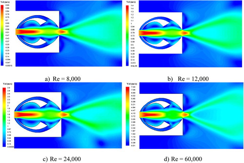
Figure 23. Contours of velocity at two times with maximum jet oscillation amplitude in the new oscillator with Re = 24,000.

Effect of turbulence model

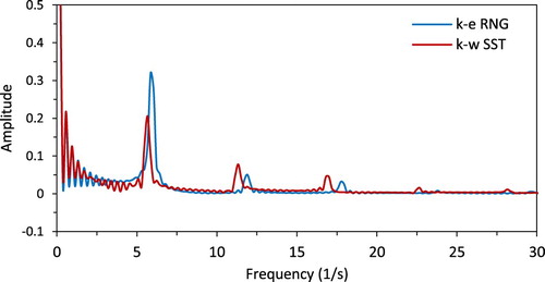
To study the effect of turbulence model on the flow of the new oscillator, another numerical solution was performed by the k-ω SST model to be compared with the k-ϵ RNG model. The results show that the flow fields predicted by the two models are very similar. Figure 24 compares the time-averaged velocity contours obtained by these two models. As can be seen, although the time-averaged flow fields are almost the same, the jet spreading angle predicted by the k-ω SST is a little less than that predicted by the k-ϵ RNG. Figure 25 compares the FFT diagram of the velocity fluctuations in the feedback channel predicted by the k-ϵ RNG and k-ω SST models. As can be seen, the k-ω SST model predicts the oscillations frequency 0.3% less than the k-ϵ RNG model.

Figure 24. Comparison of the k-ϵ RNG and k-ω SST turbulence models in predicting the time-averaged velocity contours inside and outside the oscillator.

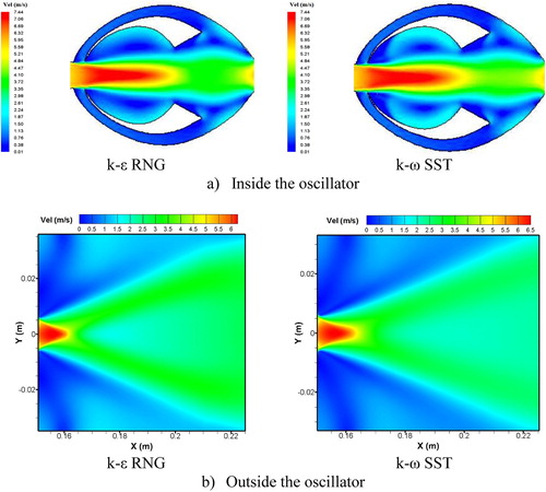
Figure 25. Comparison of the FFT diagrams of velocity fluctuations in the feedback channel predicted by the k-ϵ RNG and k-ω SST.

Effects of the design parameters for forming the oscillations

The leading throat (d₁), mid-throat (d₂), outlet throat (d₃), and the width of the feedback channel (b) are the main design parameters, which directly affect the performance of the oscillator. Each parameter has a working limit beyond which the oscillations cannot form. To prove the importance of these parameters to form the oscillations, a value beyond the working limit of each parameter was selected and a numerical solution was carried out for each selected parameter. Table 4 shows the working limit of each parameter and the values in which the oscillations did not occur. Figure 26 shows the converged velocity contours after 0.5 s, which indicates no oscillation. Figure 27 shows the FFT diagrams for the velocity fluctuations at feedback channel, which prove no oscillation with these new values of each parameter beyond the working limit.

Figure 26. Converged velocity contours after 0.5 s with the new values for each parameter.

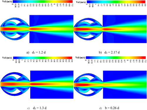
Figure 27. FFT diagrams for the velocity fluctuations at feedback channel, for new values of each parameter beyond the working limit.

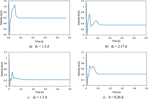
Table 4. Four main design parameters and the working limit of each parameter.

	Leading throat (d1)	Mid-throat (d2)	Outlet throat (d3)	Feedback channel width (b)
Working limit	1.1 d	2.17 d	1.14 d	0.36 d
No oscillation values	1.2 d	2.55 d	1.3 d	0.26 d

Conclusion

In this study, a novel fluidic oscillator was designed to decrease the space and oscillation amplitude inside the oscillator, and to decrease the flow rate through the feedback channel. The performance and the mechanism of oscillations in the new oscillator were evaluated by a 2D numerical solution of URANS equations with the k-ϵ RNG turbulence model. The jet flow passing through the primary and secondary chambers creates two pairs of vortices, which grow and shrink asymmetrically and start the jet oscillation. The pressure reduction inside the vortices of the primary chambers activates the feedback channels to inject the feedback flow into these vortices, which intensifies the oscillations. The interaction of the jet with the mid-throat causes a vortex to be trapped on one side of the primary chamber and returns the jet toward the other side. At the same time, a vortex inside the secondary chamber grows on one side and pushes the second half of the jet to the other side to discharge the trapped fluid in the secondary chamber into the feedback channel.

Compared to the original oscillator, the new oscillator had a continuous jet inside the primary and secondary chambers. Due to the smaller space and lower oscillation amplitude inside the new oscillator, the momentum depreciation was lower for the new oscillator. The spreading angles of the jet exiting from the two oscillators were almost the same. The frequency was increased by about 50% in the new oscillator due to its smaller size. The pressure ratio in the new oscillator was reduced by about 5%. Both mass and momentum fluxes outside the new oscillator were higher than those outside the original oscillator. The difference between the momentum fluxes of the two oscillator increased along the axial distance. The new oscillator was initially designed and evaluated by 2D numerical solution. In the future works, the geometry can be optimized to improve the performance, and PIV measurement of flow inside and outside the new oscillator can be carried out to evaluate the performance experimentally.

Disclosure statement

No potential conflict of interest was reported by the author(s).

Additional information

Funding

This work was supported by the Brain Pool Program through the National Research Foundation of Korea [grant number NRF-2019H1D3A2A01061428], which is funded by Korean Government (MSIT). Partial support was also obtained from the National Research Foundation of Korea (NRF) grant, which is funded by the Korean Government (MSIT) [grant number Nos. 2011-0030013, 2018R1A2B2007117, and 2020R1A5A8018822].

References

- Agricola, L., Hossain, M. A., Ameri, A., Gregory, J. W., & Bons, J. P. (2018). Turbine vane leading edge impingement cooling with a sweeping jet. Proceedings of the ASME Turbo Expo, 5A-2018 (pp. 1–11). https://doi.org/10.1115/GT2018-77073
- Akbarian, E., Najafi, B., Jafari, M., Ardabili, S. F., Shamshirband, S., & Chau, K. W. (2018). Experimental and computational fluid dynamics-based numerical simulation of using natural gas in a dual-fueled diesel engine. Engineering Applications of Computational Fluid Mechanics, 12(1), 517–534. https://doi.org/10.1080/19942060.2018.1472670
- Alikhassi, M., Nili-Ahmadabadi, M., Tikani, R., & Karimi, M. H. (2019). A novel approach for energy harvesting from feedback fluidic oscillator. International Journal of Precision Engineering and Manufacturing - Green Technology, 6(4). https://doi.org/10.1007/s40684-019-00128-y
- Andino, M. Y., Lin, J. C., Washburn, A. E., Whalen, E. A., Graff, E. C., & Wygnanski, I. J. (2015). Flow separation control on a full-scale vertical tail model using sweeping jet actuators. 53rd AIAA Aerospace Sciences Meeting, January. https://doi.org/10.2514/6.2015-0785
- Bobusch, B. C., Woszidlo, R., Bergada, J. M., Nayeri, C. N., & Paschereit, C. O. (2013). Experimental study of the internal flow structures inside a fluidic oscillator. Experiments in Fluids, 54(6), https://doi.org/10.1007/s00348-013-1559-6
- Breuer, M., Jovičić, N., & Mazaev, K. (2003). Comparison of DES, RANS and LES for the separated flow around a flat plate at high incidence. International Journal for Numerical Methods in Fluids, 41(4), 357–388. https://doi.org/10.1002/fld.445
- Ghalandari, M., Mirzadeh Koohshahi, E., Mohamadian, F., Shamshirband, S., & Chau, K. W. (2019). Numerical simulation of nanofluid flow inside a root canal. Engineering Applications of Computational Fluid Mechanics, 13(1), 254–264. https://doi.org/10.1080/19942060.2019.1578696
- Hossain, M. A., Prenter, R., Lundgreen, R. K., Ameri, A., Gregory, J. W., & Bons, J. P. (2017). GT2017-64479 Experimental and numerical investigation of jet film cooling. 1–13.
- Hossain, M. A., Prenter, R., Lundgreen, R. K., Ameri, A., Gregory, J. W., & Bons, J. P. (2018). Experimental and numerical investigation of sweeping jet film cooling. Journal of Turbomachinery, 140(3). https://doi.org/10.1115/1.4038690
- Jeong, H. S., & Kim, K. Y. (2018). Shape optimization of a feedback-channel fluidic oscillator. Engineering Applications of Computational Fluid Mechanics, 12(1), 169–181. https://doi.org/10.1080/19942060.2017.1379441
- Kara, K. (2017, June). Flow separation control using sweeping jet actuator. 35th AIAA Applied Aerodynamics Conference (pp. 1–10). https://doi.org/10.2514/6.2017-3041
- Kim, D., Yi, S. J., Kim, H. D., & Kim, K. C. (2017). Simultaneous measurement of temperature and velocity fields using thermographic phosphor tracer particles. Journal of Visualization, 20(2), 305–319. https://doi.org/10.1007/s12650-016-0394-2
- Kim, S. H., & Kim, H. D. (2019). Quantitative visualization of the three-dimensional flow structures of a sweeping jet. Journal of Visualization, 22, 437–447. https://doi.org/10.1007/s12650-018-00546-1
- Koklu, M. (2018). Effects of sweeping jet actuator parameters on flow separation control. AIAA Journal, 56(1), 1–11. https://doi.org/10.2514/1.J055796
- Krüger, O., Bobusch, B. C., & Paschereit, C. O. (2013, June 24–27). Numerical modeling and validation of the flow in a fluidic oscillator. 21st AIAA Computational Fluid Dynamics Conference, San Diego, CA. https://doi.org/10.2514/6.2013-3087
- Madadkon, H., Fadaie, A., & Nili-Ahmadabadi, M. (2012). Experimental and numerical investigation of unsteady turbulent flow in a fluidic oscillator flow meter with Extraction of characteristics diagrams. Modares Journal of Mechanics Engineering, 12(5), 30–42.
- Meng, Q., Chen, S., Li, W., & Wang, S. (2018). Numerical investigation of a sweeping jet actuator for active flow control in a compressor cascade. Proceedings of the ASME Turbo Expo, 2A-2018. https://doi.org/10.1115/GT201876052
- Mohammadshahi, S., Samsam-Khayani, H., Nematollahi, O., & Kim, K. C. (2020). Flow characteristics of a wall-attaching oscillating jet over single-wall and double-wall geometries. Experimental Thermal and Fluid Science, 112. https://doi.org/10.1016/j.expthermflusci.2019.110009
- Ostermann, F., Woszidlo, R., Nayeri, C. N., & Paschereit, C. O. (2015). Experimental comparison between the flow field of two common fluidic oscillator designs. 53rd AIAA Aerospace Sciences Meeting, January, 1–14. https://doi.org/10.2514/6.2015-0781
- Pandey, R. J., & Kim, K. Y. (2018). Comparative analysis of flow in a fluidic oscillator using large eddy simulation and unsteady ReynoldsAveraged Navier-Stokes analysis. Fluid Dynamics Research, 1, 1–47. https://doi.org/10.1088/1873-7005/aae946
- Ramezanizadeh, M., Alhuyi Nazari, M., Ahmadi, M. H., & Chau, K. W. (2019). Experimental and numerical analysis of a nanofluidic thermosyphon heat exchanger. Engineering Applications of Computational Fluid Mechanics, 13(1), 40–47. https://doi.org/10.1080/19942060.2018.1518272
- Seo, J. H., & Mittal, R. (2017, June). Computational modeling and analysis of sweeping jet fluidic oscillators. 47th AIAA Fluid Dynamics Conference (pp. 1–12). https://doi.org/10.2514/6.2017-3312
- Tesař, V., Zhong, S., & Rasheed, F. (2013). New fluidic-oscillator concept for flow-separation control. AIAA Journal, 51(2), 397–405. https://doi.org/10.2514/1.J051791
- Tomac, M. N. (2020). Novel jet impingement atomization by synchronizing the sweeping motion of the fluidic oscillators. Journal of Visualization, 23, 373–375. https://doi.org/10.1007/s12650-020-00632-3
- Vasta, V., Koklu, M., Wygnanski, I., & Fares, E. (2012). Numerical simulation of fluidic actuators for flow control applications (AIAA Paper, 2012(3239)).
- Woszidlo, R., Ostermann, F., Nayeri, C. N., & Paschereit, C. O. (2015). The time-resolved natural flow field of a fluidic oscillator. Experiments in Fluids, 56(6), 1–12. https://doi.org/10.1007/s00348-015-1993-8
- Xu, Y., Moon, C., Wang, J. J., Penyazkovc, O. G., & Kim, K. C. (2019). An experimental study on the flow and heat transfer of an impinging synthetic jet. International Journal of Heat and Mass Transfer, 144, 1–16. https://doi.org/10.1016/j.ijheatmasstransfer.2019.118626
- Yakhot, V., Orszag, S. A., Thangam, S., Gatski, T. B., & Speziale, C. G. (1992). Development of turbulence models for shear flows by a double expansion technique. Physics of Fluids A, 4(7), 1510–1520. https://doi.org/10.1063/1.858424