Macro-scale modeling and simulation of two-phase flow in fibrous liquid aerosol filters

Abstract

Similar to fine dust, liquid aerosols represent a risk to human health since small droplets may enter the respiratory system and cause health problems or severe diseases, such as COVID-19. Oil mist emissions from production processes and from air brakes are reduced by filters and by air dryer cartridges, respectively, while virus-like aerosols are removed by face-masks. Since the two-phase flow processes involved are highly complex and occur on vastly different scales ranging from the scale of single droplets and fibers up to the scale of a whole filter or face mask, the modeling and simulation is extremely challenging. In this work, we present a macro-scale approach for modeling and simulation of the two-phase flow processes in fibrous filters which allows predicting both pressure loss and filtration efficiency from new to steady-state where material parameters and constitutive relationships are obtained based on nano CT scans and micro-scale simulations. Compared to previous work, this approach starts from a physical basis as it relies on mass and momentum conservation and is then closed by material laws. Using this macro-scale approach it is found that both pressure loss and oil mass at steady-state are in good agreement with experimental findings.

Keywords:

• Liquid aerosol filtration
• mist filtration
• two-phase flow
• fibrous porous media
• CFD simulation

1. Introduction

Like fine dust, liquid aerosols (mist) may enter the respiratory system and cause lung cancer, allergies, asthma, or COVID-19. These mist aerosols are emitted during many industrial processes in the automotive industry like machining or from pneumatic compressors used to generate a pressure of 8–12 bars for the air brakes of trucks and busses. In order to minimize liquid aerosol emissions filters are used. The overall goal is generally to minimize pressure loss and maximize fractional separation efficiency for oil mist separators, especially for the most penetrating particle size (MPPS). The topic of aerosol filtration has recently achieved increased attention due to the COVID-19 outbreak. Often, the wearing compliance of face masks is low due to the increased breathing resistance of the masks that make longer wearing times uncomfortable. Especially, high-risk populations with chronic lung diseases and breathing problems cannot wear certified face masks due to the additional flow resistance. It is a challenge to produce well-protecting masks with high efficiency for virus-like aerosols at low-pressure drop.

While the investigation of solid aerosols (particles, fine dust) has been in the focus of research for a long time and the deposition mechanism are well known the deposition of liquid aerosols has only been investigated in depth since about 20 years. This is above all due to the extreme complexity of the flow processes. On the micro-scale, the droplets meet the fibers, form a fluid film, and coalesce to a fluid phase while they are eventually removed from the filter in a two-phase flow process where capillary and relative permeability effects are important. Furthermore, the multi-scale character, as well as the long computing times, lead to the fact that predominantly experimental work exists in this field.

In the experimental works, the evolvement of pressure loss over the filter lifetime and the evolution of fractional efficiency and its dependence on parameters like flow velocity and fluid properties have mainly been investigated (Charvet et al., 2008; Frising et al., 2004, 2005; Gu et al., 2015; Payet et al., 1992; Raynor & Leith, 2000). Partially, phenomenological models were developed based on experimental results, e.g. for pressure loss in the unloaden state and in steady-state, for effective saturation in steady-state or for the fractional efficiency of a single fiber for a defined droplet size (Charvet et al., 2008; Davies, 1952; Frising et al., 2004; Mullins et al., 2007).

In order to develop predictive models of aerosol deposition and transport, a number of authors developed CFD models, mainly based on the open-source software OpenFOAM or on the commercial software ANSYS Fluent (Chang et al., 2014; Issakhov et al., 2019; Sergi et al., 2014). Jaganathan et al. (2008) managed to obtain permeability from digital volume averaging and from solving conservation equations (no particles present) while Abishek et al. (2017) used OpenFOAM and investigated how to generate filter geometries for CFD simulations for different types of filter media. Fotovati et al. (2010) investigated the influence of fiber orientation on pressure drop and collection efficiency of solid particles by solving Stokes flow in virtual 3D geometries. Stokes flow was also solved by Hosseini and Vahedi Tafreshi (2010) who used ANSYS Fluent to calculate pressure drop and collection efficiency by implementing UDFs to account for Brownian motion and interception. Due to the typically small droplet sizes and small droplet diameters, the computational cost is very high and simulations are restricted to small parts of the model domain. However, for the determination of pressure drop of an entire filter, a model is need which is able to describe the process occurring on the scale of the whole filter (macro-scale) for varying filter geometries and materials.

Due to the innovative nature of the field of research, the complexity of the application and the multi-scale nature of the underlying processes, research using CFD simulation for liquid aerosol filtration only exists since recently. Some authors focus on single droplets, such as Gac and Gradón (2011) who studied the coalescence of two droplets and determined coalescence time depending on droplet size by means of Lattice Boltzmann simulations. King et al. (2010) developed a CFD model in OpenFoam including a particle tracking algorithm to describe the deposition of particles based on impaction, interception, and Brownian motion and validated their results by comparison to Single Fiber Efficiency theory. Mead-Hunter et al. (2013) and Mead-Hunter et al. (2011) simulated a section of a fibrous porous medium on the micro-scale using the software OpenFOAM and modeled the deposition of droplets on the fibers using a Lagrangian approach. When a grid cell is entirely filled by particles they treat it as a volume of fluid (VOF) cell and mass and momentum source terms are calculated. Thus, also the coalescence of the liquid could be described. King et al. (2010) used a similar approach, introduced four initial droplets in a rectangular grid of fibers and studied droplet collection and coalescence. Similar to solid aerosol filtration, the micro-scale simulations describing liquid aerosol filtration are restricted to very small parts of a filter due to long computational time. This again emphasizes the need for a macro-scale approach that allows for CFD simulations on the scale of an entire filter.

Therefore, a volume-averaged description is proposed in this work where no single fibers, but volume-averaged quantities such as porosity, permeability, or saturations are considered and new constitutive relationships like the capillary pressure – saturation and relative permeability–saturation relationships come into play. The development of numerical models for multi-phase flow on this macro-scale started in the 1960s in petroleum engineering, see e.g. Aziz and Settari (1979). The main goal in this field was the numerical simulation of thermally enhanced petroleum extraction, which was put into practice by means of steam injection. A good overview of the models and the underlying concept can be found, e.g. in Lake (1989) and Peaceman (1977). Multi-phase flow models for environmental problems were developed later (Feuring et al., 2014; Helmig, 1997; Liu, 2013; Niessner et al., 2011; Niessner & Hassanizadeh, 2009a, 2009b, 2011; Pop et al., 2009). Concerning a multi-scale two-phase flow approach, Piller et al. (2013) developed a workflow how to obtain permeability as well as the relative-permeability–saturation relationship from μCT scans. In the work of Hall et al. (2016), liquid aerosol transport through a porous medium was studied both experimentally and by a macro-scale two-phase flow model in the context of soil remediation using soybean oil as the dispersed phase. Liu (2013) developed a three-dimensional code based on OpenFOAM to model flow in the unsaturated zone of the subsurface based on the Richards equation. This equation is similar to the macro-scale two-phase flow equations used in this work. The main difference is, that in the Richards equation, the air phase is assumed to be infinitely mobile. To the best of our knowledge, no macro-scale two-phase flow model for liquid aerosol filtration based on conservation equations along with material parameters and constitutive relationships determined from CT scans and micro-scale simulations has been presented in the literature so far.

To account for the challenges described, our approach is as follows: From nano CT scans of current filter materials micro-scale CAD geometries of the real fibrous media are generated by means of image processing, see Figure 1. Based on these geometries, macro-scale parameters and constitutive relationships are determined. They include porosity, permeability as well as relative permeability – saturation relationships, and the capillary pressure – saturation relationship.

Figure 1. Workflow from nano CT scans to validated macro-scale simulation or liquid aerosol filtration.

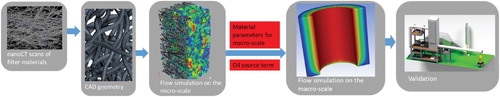
These macro-scale parameters and constitutive relationships enter the CFD simulations on the macro-scale where no droplets and fibers are resolved any more. Instead, averaged parameters are used (e.g. porosity, oil and air saturation in a cell). Therefore, the complete filter can now be considered and the pressure loss across the filter can be determined. The macro-scale model will serve as a basis for optimization of the filter setup in the future (several layers, alternating coarse, fine, oleophilic, and oleophobic layers) in order to reduce pressure loss and thus, energy needs. The optimum filter can then be produced as a physical prototype.

Unlike previous models for macro-scale two-phase flow in oil mist filters, our approach is based on fundamental conservation laws for mass and momentum along with material laws which are obtained based on nano CT scans of the real fibrous filter material. While the formerly introduced phenomenological models such as the Davies equation are restricted to a fixed and simple geometry (usually flat sheets), our approach allows us to consider arbitrary filter geometries. For example, the model introduced could also be extended to pleated filters in the future.

The purpose of this work is

• to model two-phase flow during oil mist filtration by parameters and constitutive relationships generated on the real fibrous structure and implement an oil source term accounting for droplet deposition and oil phase formation;

• to set up simulations of a real filter and determine pressure loss in the new filter and at steady-state;

• to compare the simulation results of pressure drop in the new filter and at steady-state given by our model to experimental data.

This paper is organized as follows: In Section 2, we present the equation system accounting for two-phase flow including mist deposition on the macro-scale. Next, in Section 3, we present the setup of our numerical system including how parameters and constitutive relationships are determined based on nano CT scans while in Section 4, we compare results of our simulation model to experimental data. In Section 5, we draw conclusions and give an outlook on future work.

2. Basic equations

The macro-scale model for incompressible two-phase flow in porous media consists of two mass balance equations, one for each phase α – wetting-phase ‘w’ and non-wetting phase ‘n’ – where the extended Darcy's law has been inserted ensuring momentum balance (Helmig, 1997; Peaceman, 1977), see Equations (1(1) $\begin{array}{rl}\varphi \frac{\mathrm{\partial }{S}_w}{\mathrm{\partial }t}-\mathrm{\nabla }\cdot \left(\frac{k_{rw}(S_w)}{{\mu }_w}K(\mathrm{\nabla }{p}_w-{\rho }_{w}g)\right)& =Q_w,\end{array}$(1) ) and (2(2) $\begin{array}{rl}\varphi \frac{\mathrm{\partial }{S}_n}{\mathrm{\partial }t}-\mathrm{\nabla }\cdot \left(\frac{k_{rn}(S_n)}{{\mu }_n}K(\mathrm{\nabla }{p}_n-{\rho }_{n}g)\right)& =0,\end{array}$(2) ), (1) $\begin{array}{rl}\varphi \frac{\mathrm{\partial }{S}_w}{\mathrm{\partial }t}-\mathrm{\nabla }\cdot \left(\frac{k_{rw}(S_w)}{{\mu }_w}K(\mathrm{\nabla }{p}_w-{\rho }_{w}g)\right)& =Q_w,\end{array}$(1) (2) $\begin{array}{rl}\varphi \frac{\mathrm{\partial }{S}_n}{\mathrm{\partial }t}-\mathrm{\nabla }\cdot \left(\frac{k_{rn}(S_n)}{{\mu }_n}K(\mathrm{\nabla }{p}_n-{\rho }_{n}g)\right)& =0,\end{array}$(2) (3) $\begin{array}{rl}{S}_w+S_n& =1,\end{array}$(3) (4) $\begin{array}{rl}{p}_c(S_w)& =p_n-p_w.\end{array}$(4) Here, φ is porosity, $S_{\alpha }$ the saturation, $k_{r\alpha }$ the relative permeability of phase α, and K is the intrinsic (absolute) permeability tensor. Furthermore, $Q_w$ is the source term of the wetting phase modeling the deposition rate of the wetting phase (often oil) on the fibers, ${\mu }_{\alpha }$ is the dynamic viscosity and ${\rho }_{\alpha }$ the density of phase α. Finally, $p_c$ is capillary pressure. The system of balance equations is closed by the consistency condition given in Equation (3(3) $\begin{array}{rl}{S}_w+S_n& =1,\end{array}$(3) ) that the phase saturations sum up to one and the capillary pressure – saturation relationship which is equal to the difference in phase pressures, see Equation (4(4) $\begin{array}{rl}{p}_c(S_w)& =p_n-p_w.\end{array}$(4) ). For the constitutive relationships between relative permeabilities and saturation as well as capillary pressure and saturation a Brooks–Corey parameterization is used, see Brooks and Corey (1964): (5) $\begin{array}{rl}{p}_c(S_w)& =p_d{S}_w^{-1/\lambda },\end{array}$(5) (6) $\begin{array}{rl}{k}_{rw}(S_w)& ={\left(\frac{S_w-S_{Rw}}{1-S_{Rw}-S_{Rn}}\right)}^{n_w},\end{array}$(6) (7) $\begin{array}{rl}{k}_{rn}(S_n)& ={\left(\frac{S_n-S_{Rn}}{1-S_{Rw}-S_{Rn}}\right)}^{n_n}.\end{array}$(7) In these Brooks–Corey equations, $p_d$ is the entry pressure, i.e. the pressure that the non-wetting phase needs in order to displace the wetting fluid from the largest pore and λ is the pore size exponent. Additionally, $S_{R\alpha }$ is the residual saturation and $n_{\alpha }$ the Corey exponent of phase α.

As mentioned above, the source term $Q_w$ accounts for the deposition of oil on the fibers. Our mid-term research goal is to derive this term from micro-scale simulations where oil droplets are represented by a Lagrangian or discrete element (DEM) approach. Currently, we use a space-dependent polynomial model for this term.

3. Setup of the numerical system

Our purpose is to set up a CFD model allowing to simulate the oil deposition and drainage in a filter cartridge from new to steady-state in order to evaluate the pressure drop. Therefore, we use ANSYS Fluent R19.1. For the filter cartridge, we also measure fractional efficiency as well as pressure drop.

In Section 3.1, we present the geometrical setup while the meshing issues are discussed in Section 3.2. In Section 3.3, we will discuss the boundary and initial conditions used and specify the flow regime in Section 3.4. Next, in Section 3.5, we show how parameters and constitutive relationships of our filter medium are obtained from nano CT scans. Then, in Section 3.6, we discuss the oil source term modeling the deposition of oil on the fibers. In Section 3.7, we give a short overview of the solvers and solver parameters used.

3.1. Geometrical setup

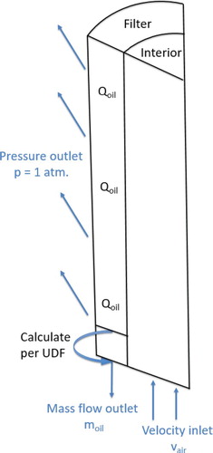
The filter cartridge used in our studies is cylindrical and has a height of 1200 mm with an outer diameter of 327 mm. The inner diameter is 195 mm, which results in a width of the filter of 66 mm, which the airflow has to pass from the inside to the outside of the filter. In our simulation, due to symmetry reasons and in order to reduce computing time, we only model 1/32 nd of the cylindrical domain (a ${11.25}^{\circ }$ section). A sketch of the system is shown in Figure 2. In order to improve convergence, the geometry is slightly simplified. Specifically, the segments of the circles are replaced by straight lines, see Figure 3. This makes the simulation not only more stable, but also significantly faster since convergence is achieved in fewer iterations. The volumetric difference between the real geometry and the simplified geometry is negligible (0.32% for both interior and filter zone). The impact of this simplification on the simulation results of interest is evaluated by comparing the pressure drop of the original and the simplified geometry. As the difference is only 0.0124%, the impact on the flow quantities of interest can be neglected.

Figure 2. Simulation domain of the filter cartridge including boundary conditions.

3.2. Mesh setup

The mesh is mainly made up of hexahedra. Towards the center of the cylinder, wedges must be used as the angle is too acute for hexahedra. While the orthogonal quality and skewness quality criterion of the hexagonal cells is excellent, the quality of the wedge cells is much worse. However, on average, the net quality is excellent, see Table 1.

Figure 3. Simplification of the cylindrical model domain leads to improved convergence.

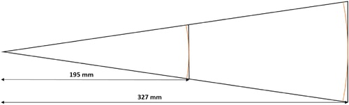
Table 1. Mesh quality statistics of the mesh used in the simulations.

	Orthogonal quality	Skewness
Minimum	0.1875	4.378e−2
Maximum	0.99979	0.8125
Average	0.98383	6.9034e−2
Standard deviation	7.2763e−2	0.10567

In order to determine a reasonable size of the grid cells, a grid convergence study is carried through using a simplified physical setup, see Figure 4. Although grid convergence was not yet completely reached a grid cell size of 3 mm was chosen as a compromise between accuracy and computing time. This results in a total of 25,551 cells and 32,494 nodes for the whole domain.

Figure 4. Pressure loss as a function of the grid cell size.

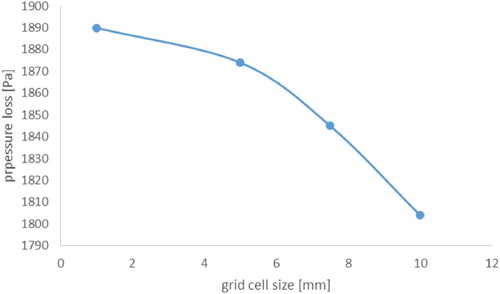
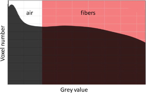
Figure 5. Histogram of voxel number depending on the gray value of the nano CT scan. The red shaded area is identified as fibers.

3.3. Boundary and initial conditions

We distinguish between two different zones. In the interior zone, an airflow of $750{\mathrm{m}}^3/\mathrm{h}$ comes in at the lower boundary via a velocity inlet. The airflow profile is imposed via a User Defined Function (UDF) which describes half of a parabolic velocity profile as an approximation. Although the flow is not laminar, see Section 3.4, this profile is good enough such that the turbulent flow in the ‘Interior’ zone will provide an accurate velocity distribution at the interface to the domain ‘Filter’.

The zone ‘Filter’ is defined to be a porous medium and thus represents the filter. On the outside of the filter a pressure boundary condition is imposed (ambient pressure). The bottom side of the filter is a mass flow outlet for oil while the mass flux of air is zero. Thus, only oil can leave this boundary (drainage). Like this, this boundary condition ensures that the oil drainage is airtight, as is the case in reality. This value is naturally rather an outcome of the model than an input. Because value for the oil flux out of the system still has to be given and is time-dependent, a UDF is used here. This UDF takes the mass flow profile of the oil of a plane located just above the lower boundary of the filter and passes this value to the boundary condition of the mass flow outlet (see Figure 2). Specifically, the function transfers the oil phase velocity profile and mass flux of the oil phase from the plane 1 mm above to the mass-flow outlet. First, the plane which transfers the profile is given an ID and both mass flux and oil velocity are set to 0 at the beginning of each iteration. After that, a macro is used to define the transfer function such that it includes the velocity profile of the oil phase at the plane. Then, this profile is read in and serves as an input parameter for the mass flux of oil at the boundary as well as for the flow direction (drainage). All other system boundaries are walls. At the initial state, the air pressure is zero ($p_n=0$) and the system is at rest ($v_{\alpha }=0$).

3.4. Flow regime

In order to determine the flow regime in ‘Interior’ and ‘Filter’ zone, respectively, the Reynolds numbers are calculated. In the ‘Interior’ zone, the inner diameter of the filter is used as the characteristic length. The mean velocity, $\overline{v}$ is calculated from the volumetric flow rate ($\dot{V}=750{\mathrm{m}}^3/\mathrm{h}$) and the cross-sectional area of the inlet, (8) $R{e}_{\mathrm{int}}=\frac{{\overline{v}}_{\mathrm{int}}\cdot d_{\mathrm{int}}}{{\nu }_{\mathrm{air}}}=\frac{6.944\mathrm{m}/\mathrm{s}\cdot 0.195\mathrm{m}}{1.46\cdot {10}^{-5}{\mathrm{m}}^2{\mathrm{s}}^{-1}}=\mathrm{92,745.}$(8) Thus, the flow in the ‘Interior’ zone is turbulent. For modeling turbulence the k- ε standard model is chosen. A comparison between different turbulence models showed minimal differences in pressure drop for the system. The maximum deviation of pressure drop from k- ε standard model was only 0.021%. These settings for the turbulent flow lead to small $y+$ values ranging from 0.234 to 0.934 at the wall (top) in the ‘Interior’ zone.

In the zone ‘Filter’ the characteristics length is given by the mean fiber diameter ($d_{\mathrm{fil}}=6\text{μ}\mathrm{m}$) and the mean flow velocity is calculated by dividing the volumetric flux by the area of the inner boundary of the zone ‘Filter’. Thus, the Reynolds number is (9) $R{e}_{\mathrm{fil}}=\frac{{\overline{v}}_{\mathrm{fil}}\cdot d_{\mathrm{fil}}}{{\nu }_{\mathrm{air}}}=\frac{0.176\mathrm{m}/\mathrm{s}\cdot 6\cdot {10}^{-6}\mathrm{m}}{1.46\cdot {10}^{-5}{\mathrm{m}}^2{\mathrm{s}}^{-1}}=0.072$(9) and the flow is creeping (Re<1) allowing to use Darcy's law in the porous medium.

3.5. Parameters and constitutive relationships

In this section, we describe how to obtain voxel geometries from nano CT scans of actual filter materials by means of image analysis and how, in the end, we come up with parameters and constitutive relationships that are needed for the macro-scale CFD simulations.

In the first step, nano CT scans were generated from the filter material currently used in oil mist filters, see Figure 5. The filter material considered in this work is made up of glass fibers and can be considered homogeneous. The scanned section was $1.2\cdot 1.2\cdot 0.7{\mathrm{mm}}^3$ in total. The resolution of this nano CT scans was set to $0.3\text{μ}\mathrm{m}$ per pixel allowing to visualize fibers down to $1\text{μ}\mathrm{m}$. 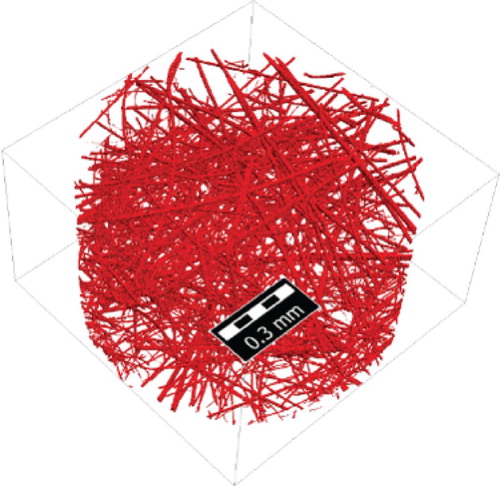The next step is the generation of a voxel geometry. Therefore, all slices of the CT scan are imported into the software program GeoDict. By applying a grey-value threshold, each pixel in the CT scan can be assigned to be air or fiber (glass), see Figure 5.The pixels get the third dimension as all slices are put one behind the other to form a stack, see Figure 6. Since the nano CT image consists of unconnected gray values only and often contains noise, this noise is removed by using a Gaussian filter. After that, some connectivity is established by using morphological opening and morphological closing. A detailed description of this methodology how to obtain a 3D geometry of a filter medium based on CT scans is described in Lehmann et al. (2016). The resulting geometry is shown in Figure 7.

Figure 6. Stacked nano CT scans are used to generate a 3D picture of the scanned filter medium.

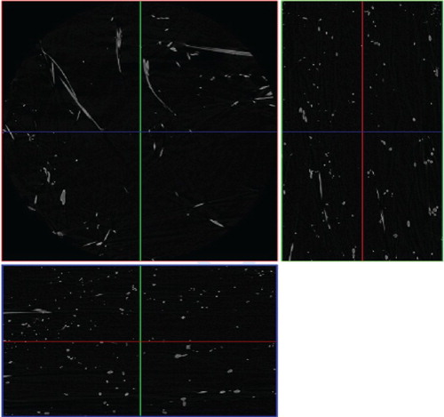
Figure 7. Voxel-based geometry of the fibrous porous medium.

The macro-scale parameters K and φ and the constitutive relationships $p_c(S_w)$ and $k_{r\alpha }(S_{\alpha })$ occurring in Equation (1(1) $\begin{array}{rl}\varphi \frac{\mathrm{\partial }{S}_w}{\mathrm{\partial }t}-\mathrm{\nabla }\cdot \left(\frac{k_{rw}(S_w)}{{\mu }_w}K(\mathrm{\nabla }{p}_w-{\rho }_{w}g)\right)& =Q_w,\end{array}$(1) ) through (4(4) $\begin{array}{rl}{p}_c(S_w)& =p_n-p_w.\end{array}$(4) ) are determined based on the geometry obtained from nano CT scans. While φ is obtained based on the geometry only, K, $p_c(S_w)$, and $k_{r\alpha }(S_{\alpha })$ are determined from micro-scale simulations. The intrinsic (or absolute) permeability K is obtained by solving the single-phase steady Stokes equation using the explicit jump flow solver that is appropriate for porous media with large porosities. Due to the small Reynolds number (Re<1), the flow is in the Darcy regime, i.e. pressure drop and specific flux (Darcy velocity) are proportional to one another, see Section 3.4. This flow regime is called ‘creeping flow’. As boundary conditions on the micro-scale flow domain (top and bottom of the cylinder shown in Figure 7, the Darcy velocity (specific flux) is given. The side boundaries are closed. The micro-scale simulations then yield the pressure drop across the porous medium. Knowing Darcy velocity and pressure drop, the intrinsic permeability tensor K is calculated and transformed to diagonal form using principal axis transformation.

Both capillary pressure – saturation and relative permeability – saturation relationships are obtained by a sequence of quasi-steady two-phase flow states each corresponding to a different saturation of the two phases. For the $p_c(S_w)$ relationship, the pore morphology method is used, also known as the method of ‘maximum inscribed spheres’. Here, $p_n$ and $p_w$ are given as boundary conditions on top and bottom boundaries of the micro-scale model domain shown in Figure 7 while the side boundary is closed. Since our filter is made up of glass fibers, oil is the wetting-phase w while air is the non-wetting phase n. The interfacial tension between oil and air is needed as an input. Capillary pressure, given by the difference $p_n-p_w$ across the domain, is then increased stepwise, by increasing $p_n$. For each capillary pressure, the steady-state distribution of the two phases is calculated, which yields one point of the $p_c-S_w$ relationship.

For obtaining the relative permeability–saturation relationship, the two-phase Darcy equation is solved for different saturation levels, similar to what is described for the calculation of K above. Knowing K, the reduction factor of the intrinsic permeability known as the relative permeability (between 0 and 1) can then be calculated. The porosity φ is the easiest parameter since it can be obtained geometrically as the volume fraction of void space in the porous medium.

All simulations were carried through using the commercial software GeoDict along with the modules MatDict, FlowDict, and SatuDict. The parameters of the Brooks–Corey parameterization have been fitted using gnuplot. Various authors have investigated the quality of macro-scale parameters using GeoDict and found them to be close to the experimental of analytical data. Ali et al. (2020), e.g. obtained intrinsic permeabilites for fiber reinforcements based on CT scans and GeoDict simulations. They found them to be in good agreement with experimental data. Jaganathan (2009) also obtained intrinsic permeabilities from CT scans for fibrous filters and found them to be in good agreement with analytical solutions. Furthermore, Bai et al. (2020) showed that pore-size distribution obtained by GeoDict agrees well with experimental data. Interfacial tension as an input parameter and all output parameter values are given in Table 2.

Table 2. Material parameters used in the CFD simulations.

Parameter	Symbol	Value
Interfacial tension	σ	0.025 N/m
Porosity	φ	0.985
Intrinsic permeability
– Flow direction	$K_{xx}$	$3.01\cdot {10}^{-10}{\mathrm{m}}^2$
– Drainage direction	$K_{zz}$	$5.56\cdot {10}^{-10}{\mathrm{m}}^2$
Corey exponent of air	$n_n$	2.2
Residual saturation of air	$S_{Rn}$	0.6
Corey exponent of oil	$n_w$	3.6
Residual saturation of oil	$S_{Rw}$	0.12
Entry pressure	$p_d$	1440 Pa
Pore size exponent	λ	2.17

3.6. Source term

Since on the macro-scale we use an averaged approach, we cannot represent oil droplets entering the filter through an inlet. Instead, we model the oil deposition on the fibers by a source term (UDF). This source term will finally be determined from micro-scale simulations and will probably depend on flow velocity, saturation and other parameters. Since this is an extremely challenging and time-consuming task, we use a phenomenological ‘dummy’ function in the meantime which we try to keep as simple as possible.

This function ensures (i) that the average drainage rate of oil is approximately in agreement with the mass flux of mist applied to the filter and (ii) that the inhomogeneous oil deposition along the flow path is described. Close to the inlet, large droplets are deposited while towards the outlet, smaller and smaller droplets accumulate on the fibers. Thus, the oil source term is not constant across the filter, but a monotonically decreasing function. We currently assume it to be a polynomial function of the third order. Because the origin of the coordinate system is located on the symmetry axis of the domain, the x-coordinate is sufficient to describe the position within the UDF. Specifically, our function is (10) $\begin{array}{rl}{Q}_w\left[\frac{\mathrm{kg}}{{\mathrm{m}}^3\mathrm{s}}\right]& =-0.88343\cdot x^3+0.41194\cdot x^2-0.06445\cdot \\ & x+\mathrm{0.00339.}\end{array}$(10) As mentioned above, this function is meant as a starting point as long as a source term determined by micro-scale simulations has not been developed yet. Since this preliminary source term only depends on space, the deposition rate does not change with time and is especially not dependent on oil saturation. Although this is a restriction, for simplicity reasons, we decided to stick to this preliminary source term depending on space only.

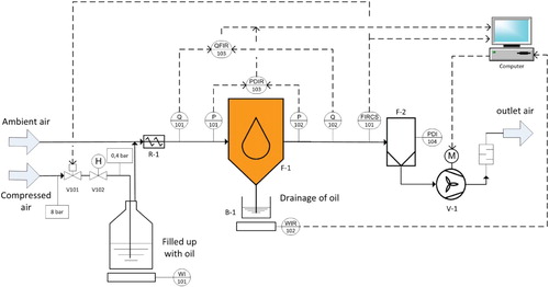
Figure 8. CAD picture of the test bench used to determine pressure drop and (fractional) efficiency.

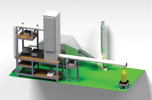
Figure 9. Flow diagram of the test bench.

3.7. Solver parameters

The system of balance equation is solved by a phase-coupled SIMPLE scheme. For space discretization, a least-squares cell-based method is used with first-order upwinding for the momentum balance equations and the ‘QUICK’ method for the discretization of the volume fractions. A first-order implicit approach is used for time discretization with a time step between 0.01 and 0.025 s. Since the default settings of the under-relaxations factors (URF) do not give a stable simulation of the system, they are reduced. The URF for the momentum equation is set to 0.5 (default value 0.7) and the URF for volume fraction is set to 0.35 (default value 0.5).

4. Simulation and comparison to experimental results

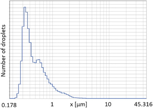
For determining experimental values of pressure loss and (fractional) efficiency the filter cartridge is clamped into a measuring cell and connected to an aerosol generator (Topas ATM 241), high-pressure ventilator (Elektror HRD 2 T FUK-95/3,0), and HEPA filter. The aerosol generator Topas ATM 241 is filled by Cutmax oil and operated by compressed air. Aerosol droplets are generated based on the venturi effect. The large droplets are separated in a ${90}^{\circ }$ bend due to inertia. The droplet size distribution was measured with an aerosol spectrometer Palas PROMO 3000 with two Palas Welas aerosol sensors upstream and downstream of the filter. Thus, a quasi-simultaneous measurement of the droplet size distributions was possible in order to calculate fractional filtration efficiency accurately. The setup of the test bench is shown in Figures 8 and 9. The ventilator is connected downstream and the air is sucked through the filter. The ventilator is preceded by a HEPA filter to completely separate the remaining oil from the outgoing air. The aerosol generator produces a droplet size distribution as shown in Figure 10. The aerosol and pressure sensors are located immediately before and after the measuring cell. The measurement data is sent to a laptop during a test run and recorded. For the purpose of continuously monitoring the drainage rate, a balance (Kern PNS 3000-2) is placed under the aerosol generator and the collecting basin of the oil drain and the mass measurements are also sent to the laptop.

Figure 10. Example of a measured droplet size distribution.

4.1. Pressure drop of a new filter

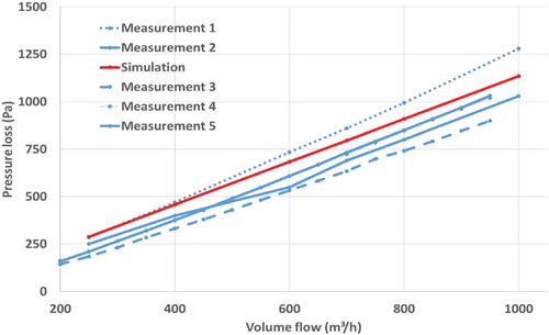
As a first part of the comparison, the measured pressure losses of five different, but identically manufactured, cartridges in the new (i.e. unsaturated) state at different volume fluxes are compared to the respective simulation results. Here, it can already be seen that there is a significant difference between the pressure losses of the filter cartridges observed in the experiments. This results from the variability of the material properties and of the production process, which also became evident when measuring the basis weight of the filter material (maximum difference of approximately 25% for eight different filter samples). This has the consequence that there are differences in permeability and thus in the pressure losses between the filters. Nonetheless, the pressure loss predicted by the simulations and the measurements results is generally in good agreement (Figure 11). This is remarkable since for this (single-phase) case all parameters in the simulation were based on data obtained from the nano CT scans and no fitting was done.

Figure 11. Pressure loss of unsaturated filter cartridges – experimental vs. simulation results.

4.2. Pressure drop as a function of time during oil loading

Next, the (unsteady) loading phase of the filter is considered until steady state is reached, see Figure 12. Therefore, a constant volumetric flux of $750{\mathrm{m}}^3/\mathrm{h}$ is applied. Failure of the power supply leads to the fact that some data in the curve was missing. Still, it is evident that steady-state is reached after about 200 h. The steady-state pressure loss increase with respect to the initial pressure loss is at around 520 Pa. The average mass flux of oil mist produced by the aerosol generator was determined as 48 g/h with variability of around 10%. The recording time of the pressure loss at the test bench was approximately 600 h.

Figure 12. Pressure loss over time determined by simulations and experimentally at a volumetric flow rate of $750{\mathrm{m}}^3/\mathrm{h}$.

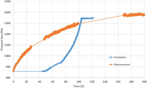
Since the computational cost of the simulation is high, the simulation had to be accelerated. In order to do so, we applied an initial oil saturation in the first third of the filter thickness (behind the inlet) that is equal to the residual oil saturation of 0.12. As the oil phase is still not mobile, the pressure loss increase after this initial loading is still zero. The oil mass corresponding to the initial saturation was calculated and from that and the oil mass flux a time ‘shift’ of around 44.6 h between simulation and experiment was determined. The simulation converged generally after 1 inner iteration, but shortly before reaching steady-state, 25 inner iterations were needed for convergence within a time step. A time step size of 0.01 s in the initial phase of the simulation where convergence was reached after one iteration led to a simulated time of 42 s for each second the Simulation runs, calculated with two Intel Xeon Gold 6126 and 24 logical processors'. The simulation was stopped at 120 h of simulated time since from visual inspection, the pressure loss determined by simulation did not change as a function of time any more. Thus, it was supposed that steady-state was reached in the simulation.

In Figure 12, we observe the typical exponential pressure increase in the experiment (accumulation stage). As the oil saturation increases within the filter the collection efficiency changes. In the simulation, we used a phenomenological source term to account for collection efficiency. As this source term is meant as a first step to set up and test our macro-scale model we tried to keep it as simple as possible. Thus, this source term only depends on space but not on time. Therefore, the collection efficiency remains constant during the filter lifetime. Especially, it does not change as oil saturation increases. Although this is a simplification, of course, we tried to keep our model simple and not add too much complexity in this first step. This obviously leads to the fact that during the loading phase of the filter as the oil saturation increases, differences between experimental and simulation results occur. Despite these differences, the general agreement of simulation and experimental pressure loss increase, especially in steady-state, is good (1346 Pa in the simulation compared to 1372 Pa in the experiment).

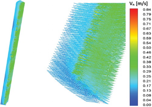
Also, the oil mass in the filter at steady-state is compared. While the oil mass determined by simulations was equal to 5.12 kg, a steady-state oil mass of 4.98 kg was measured in the experiment. This is especially remarkable since the simulation was carried through with a source term that is not yet obtained from micro-scale simulations (see Section 3.6) and the filter material itself has fluctuations. The oil saturation above the capillary fringe, the air pressure in the filter, and the air velocity vectors in the filter at steady state, respectively, are shown in Figures 13– 15. While on the left-hand side of these figures, a 2d vertical plane section through the filter is shown, a zoomed and 3d view of the lower end of the filter is shown situated just above the capillary fringe. Air pressure decreases from 1348 Pa at the inlet to 0 Pa (atmospheric pressure) at the outlet as could be expected. The oil saturation above the capillary fringe shows a clear horizontal profile (high saturation at the inlet, low saturation at the outlet). However, the vertical oil movement (drainage due to gravity) does not influence the vertical saturation profile strongly.

Figure 13. Steady-state oil saturation on a vertical plane section through the filter (left-hand side) and detailed 3d view (right-hand side) of the lower end of the filter above the capillary fringe. The CFD simulation was carried through at a volumetric flux of $750{\mathrm{m}}^3/\mathrm{h}$.

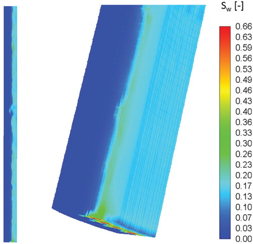
Figure 14. Steady-state air pressure on a vertical plane section through the filter (left-hand side) and detailed 3d view (right-hand side) of the lower end of the filter above the capillary fringe. The CFD simulation was carried through at a volumetric flux of $750{\mathrm{m}}^3/\mathrm{h}$.

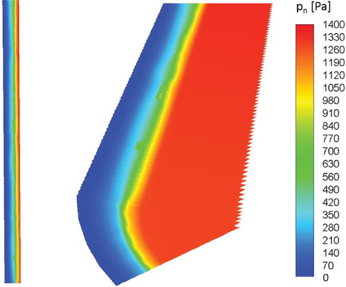
Figure 15. Steady-state air velocity vectors on a vertical plane section through the filter (left-hand side) and detailed 3d view (right-hand side) of the lower end of the filter above the capillary fringe. The CFD simulation was carried through at a volumetric flux of $750{\mathrm{m}}^3/\mathrm{h}$.

5. Summary and outlook

The purpose of this work was to present a macro-scale approach for modeling oil mist filtration and to develop a macro-scale two-phase flow model to predict the pressure loss of an existing industrial oil mist filter from new to steady-state. For this purpose, the physical basics, model assumptions and processes in the filter were presented. Unlike previous phenomenological or empirical models, our approach relies on fundamental conservation laws of mass and momentum along with constitutive relationships. Subsequently, the setup of the CFD simulations was described including boundary conditions, dimensions, solver parameters, an oil source term accounting for deposition, and how an airtight oil drainage condition is created. After that, the simulation results of pressure loss in new and steady-state were compared to experimental data. The pressure loss predicted by our model is in good agreement with the results obtained from experiments. Both in the initial state and during the loading of the filter, the simulated and measured results are rather close. Limitations of the presented model concern mainly the oil source term which is currently phenomenological in nature and should finally be based on micro-scale simulations where the deposition and re-entrainment of oil droplets are determined as a function of saturation and flow velocity. Furthermore, many of the highly complex micro-scale phenomena like droplet coalescence, breakup, or film flow occur before the macro-scale residual saturation is reached. The macro-scale two-phase flow processes, contrarily, only start when the residual saturation is exceeded. Thus, our model is limited to oil saturations larger than the residual saturation and describes the flow of oil and air phase driven by capillary forces, gravity, and pressure gradients.

Future directions of research focus on developing a micro-scale model for simulating droplet movement, deposition, and re-entrainment on the micro-scale depending on oil saturation and flow velocity. This will finally allow us to determine the oil source term locally and more physically based. Subsequently, the macro-scale model should be applied to different filter materials and geometries for validation. In addition, this work may serve as a basis for the optimization of filter cartridges. Specifically, the optimum layering of the filter with respect to pressure loss and separation efficiency will be determined with respect to design parameters, such as permeability and entry pressure of each layer. Once the optimal setup has been found, a prototype will be constructed and the simulations will be validated by comparison to measurement results using this prototype. Further improvements are expected by using pleated filters. Again, our model can be used to investigate the optimum number of pleats, filter thickness and material. Furthermore, our model can be applied in order to optimize other liquid aerosol filter applications, such as COVID-19 face masks, air dryer cartridges of braking systems, or filter cartridges for compressed air.

Acknowledgments

This work was funded by the federal state of Baden-Württemberg and the ‘European Regional Development Fund’ (EFRE), Vorhaben: High-Tech-Aerosolnebelabscheider im Zero-Design (HAAZ) FKZ: 1096283. We thank Junker-Filter GmbH for fruitful discussions and for providing us with filter cartridges. Furthermore, we are grateful to Math2Market for their generous support of our work.

Disclosure statement

No potential conflict of interest was reported by the author(s).

Additional information

Funding

This work was funded by the federal state of Baden-Württemberg and the ‘European Regional Development Fund’ (EFRE), Vorhaben: High-Tech-Aerosolnebelabscheider im Zero-Design (HAAZ) FKZ: 1096283.

References

- Abishek S., King A., Mead-Hunter R., Golkarfard V., Heikamp W., & Mullins B. (2017). Generation and validation of virtual nonwoven, foam and knitted filter (separator/coalescer) geometries for CFD simulations. Separation and Purification Technology, 188, 493–507. https://doi.org/10.1016/j.seppur.2017.07.052
- Ali, M., Umer, R., & Khan, K. (2020). A virtual permeability measurement framework for fiber reinforcements using micro CT generated digital twins. International Journal of Lightweight Materials and Manufacture, 3(3), 204–216. .https://doi.org/10.1016/j.ijlmm.2019.12.002.
- Aziz K., & Settari A. (1979). Petroleum reservoir simulation. Elsevier Applied Science.
- Bai H., Qian X., Fan J., Qian Y., Duo Y., Liu Y., & Wang X. (2020). Computing pore size distribution in non-woven fibrous filter media. Fibers and Polymers, 21(1), 196–203. https://doi.org/10.1007/s12221-020-9181-8
- Brooks R., & Corey A. (1964, January). Hydraulic properties of porous media. Hydrology Paper, 7, 26–28.
- Chang C., Chan C C., Cheng K J., & Lin J. (2014). Computational fluid dynamics simulation of air exhaust dispersion from negative isolation wards of hospitals. Engineering Applications of Computational Fluid Mechanics, 5(2), 276–285. https://doi.org/10.1080/19942060.2011.11015370
- Charvet A., Gonthier Y., Bernis A., & Gonze E. (2008). Filtration of liquid aerosols with a horizontal fibrous filter. Chemical Engineering Research and Design, 86, 569–576. https://doi.org/10.1016/j.cherd.2007.11.008
- Davies C. (1952). The separation of airborne dust and particle. Proceedings of the Institution of Mechanical Engineers, 167(1b), 185–199. https://doi.org/10.1177/002034835316701b13
- Feuring, T., Braun, J., Linders, B., Bisch, G., Hassanizadeh, S., & Niessner, J. (2014). Horizontal redistribution of two fluid phases in a porous medium: Experimental investigations. Transport in Porous Media, 105, 503–515. https://doi.org/10.1007/s11242-014-0381-9.
- Fotovati S., H. Vahedi Tafreshi, & Pourdeyhimi B. (2010). Influence of fiber orientation distribution on performance of aerosol filtration media. Chemical Engineering Science, 65, 5285–5293. https://doi.org/10.1016/j.ces.2010.06.032
- Frising T., Gujisaite V., Thomas D., Callé S., Bémer D., Contal P., & Leclerc D. (2004). Filtration of solid and liquid aerosol mixtures. Filtration & Separation, 41(2), 37–39. https://doi.org/10.1016/S0015-1882(04)00076-X
- Frising T., Thomas D., Bémer D., & Contal P. (2005). Clogging of fibrous filters by liquid aerosol particles: Experimental and phenomenological modelling study. Separation and Purification, 60, 2751–2762. https://doi.org/10.1016/j.ces.2004.12.026
- Gac J., & Gradón L. (2011). A two-dimensional modeling of binary coalescence time using the two-color lattice-Boltzmann method. Journal of Aerosol Science, 42, 355–363. https://doi.org/10.1016/j.jaerosci.2011.02.004
- Gu Q., Henderson R., & Tatarchuk B. (2015). A CFD pressure drop model for microfibrous entrapped catalyst filters using micro-scale imaging. Engineering Applications of Computational Fluid Mechanics, 9(1), 567–576. https://doi.org/10.1080/19942060.2015.1094415
- Hall R., Murdoch L., Falta R., Looney B., & Riha B. (2016). Evaluation of liquid aerosol transport through porous media. Journal of Contaminant Hydrology, 190, 15–28. https://doi.org/10.1016/j.jconhyd.2016.03.003
- Helmig R. (1997). Multiphase flow and transport processes in the subsurface: A contribution to the modeling of hydrosystems. Springer.
- Hosseini S., & Vahedi Tafreshi H. (2010). Modeling particle filtration in disordered 2-D domains: A comparison with cell models. Separation and Purification Technology, 74, 160–169. https://doi.org/10.1016/j.seppur.2010.06.001
- Issakhov A., Bulgakov R., & Zhandaulet Y. (2019). Numerical simulation of the dynamics of particle motion with different sizes. Engineering Applications of Computational Fluid Mechanics, 13(1), 1–25. https://doi.org/10.1080/19942060.2018.1545253
- Jaganathan S. (2009). An investigation on fluid flow in fibrous materials via image-based fluid dynamics simulations [Unpublished doctoral dissertation]. State University. https://repository.lib.ncsu.edu/handle/1840.16/5861NC
- Jaganathan S., Vahedi Tafreshi H., & Pourdeyhimi B. (2008). A realistic approach for modeling permeability of fibrous media: 3-D imaging coupled with CFD simulation. Chemical Engineering Science, 63, 244–252. https://doi.org/10.1016/j.ces.2007.09.020
- King A., Mullins B., & Lowe A. (2010, December 12). Discrete particle tracking in fluid flows for particulate filter simulations. In K. Teh, I. Davies, & I. Howard (Eds.), 6th Australasian congress on applied mechanics. Engineers Australia.
- Lake L. (1989). Enhanced oil recovery. Prentice Hall.
- Lehmann M., Weber J., Kilian A., & Heim M. (2016). Microstructure simulation as part of fibrous filter media development processes – from real to virtual media. Chemical Engineering & Technology, 39(3), 403–408. https://doi.org/10.1002/ceat.v39.3 doi: 10.1002/ceat.201500341
- Liu X. (2013). Parallel modeling of three-dimensional variably saturated ground water flows with unstructured mesh using open source finite volume platform OpenFOAM. Engineering Applications of Computational Fluid Mechanics, 7(2), 223–238. https://doi.org/10.1080/19942060.2013.11015466
- Mead-Hunter R., King A., Kasper G., & Mullins B. (2013). Computational fluid dynamics (CFD) simulation of liquid aerosol coalescing filters. Journal of Aerosol Science, 61, 36–49. https://doi.org/10.1016/j.jaerosci.2013.03.009
- Mead-Hunter, R., Mullins, B., & King, A. (2011). Development and validation of a computational fluid dynamics (CFD) solver for droplet-fibre systems, in Chan, F. and Marinova, D. and Anderssen, R.S. (ed), MODSIM2011: 19th International Congress on Modelling and Simulation, Dec 12-16 2011. Perth, WA: Modelling and Simulation Society of Australia and New Zealand.
- Mullins B., Braddock R., & Kasper G. (2007). Capillarity in fibrous filter media: Relationship to filter properties. Chemical Engineering Science, 62, 6191–6198. https://doi.org/10.1016/j.ces.2007.07.001
- Niessner J., Berg S., & Hassanizadeh S. (2011). Comparison of two-phase Darcy's law with a thermodynamically consistent approach. Transport in Porous Media, 88, 133–148. https://doi.org/10.1007/s11242-011-9730-0
- Niessner J., & Hassanizadeh S. (2009a). Modeling kinetic interphase mass transfer for two-phase flow in porous media including fluid-fluid interfacial area. Transport in Porous Media, 80, 329–344. https://doi.org/10.1007/s11242-009-9358-5
- Niessner J., & Hassanizadeh S. (2009b). Non-equilibrium interphase heat and mass transfer during two-phase flow in porous media – theoretical investigations and modeling. Advances in Water Resources, 32, 1756–1766. https://doi.org/10.1016/j.advwatres.2009.09.007
- Niessner J., & Hassanizadeh S. (2011). Mass and heat transfer during two-phase flow in porous media – theory and modeling. In Mass transfer. In Tech Open Access Publisher.
- Payet S., Boulad D., Madelaine G., & Renoux A. (1992). Penetration and pressure drop of a HEPA filter during loading with submicron liquid particles. Journal of Aerosol Science, 23(7), 723–735. https://doi.org/10.1016/0021-8502(92)90039-X
- Peaceman D. (1977). Fundamentals of numerical reservoir simulation. Elsevier Applied Science.
- Piller, M., Casagrande, D., Schena, G., & Santini, M. (2013). Pore-scale simulation of laminar flow through porous media. Journal of Physics: Conference Series, 501, 012010. https://doi.org/10.1088/1742-6596/501/1/012010.
- Pop I., van Duijn C., Niessner J., & Hassanizadeh S. (2009). Horizontal redistribution of fluids in a porous medium: The role of interfacial area in modeling hysteresis. Advances in Water Resources, 32, 383–390. https://doi.org/10.1016/j.advwatres.2008.12.006
- Raynor P., & Leith D. (2000). The influence of accumulated liquid on fibrous filters. Journal of Aerosol Science, 31(1), 19–34. https://doi.org/10.1016/S0021-8502(99)00029-4
- Sergi D., Grossi L., Leidi T., & Ortona A. (2014). Surface growth effects on reactive capillary-driven flow: Lattice Boltzmann investigation. Engineering Applications of Computational Fluid Mechanics, 8(4), 549–561. https://doi.org/10.1080/19942060.2014.11083306