Heat transfer through converging-diverging channels using Adomian decomposition method

Abstract

This study consists of proposing a new mathematical method to develop a new model for evaluating thermal distributions throughout convergent-divergent channels between non-parallel plane walls in Jeffery Hamel flow. Subsequently, dimensionless equations that govern temperature fields and velocity are numerically tackled via the Runge–Kutta-Fehlberg approach based on the shooting method. Additionally, an analytical study is performed by applying an effective computation technique named Adomian Decomposition Method. Determining the effect of Reynolds and Prandtl numbers on the heat transfer and fluid velocity inside converging/diverging channels can be mentioned as the fundamental purpose of this research. Based on the results obtained for dimensionless velocity and thermal distributions, a supreme match can be observed between numerical and analytical results indicating the adopted ADM method is valid, applicable, and has great precision.

KEYWORDS:

• Fluid flow
• heat transfer
• inclined walls
• Adomian Decomposition method
• numerical solution

Nomenclature

Symbol Definition

a	=	Constant
b	=	Constant
d	=	Thermal diffusivity
An	=	Adomian polynomials
Bn	=	Adomian polynomials
Cp	=	Specificheat of studied fluids, J/Kg.°K
f	=	Function
F	=	Dimensionless velocity
Fn	=	Solution terms for velocity
g	=	Function
G	=	Dimensionless temperature
Gn	=	Solution terms for temperature
K	=	Thermal conductivity, W/m.°K
Nu	=	Nonlinear velocity
Ng	=	Nonlinear temperature
P	=	Fluid pressure,N/m2
Pr	=	Prandtl number
Q	=	Volume flux
r	=	Radial coordinate, m
Re	=	Reynolds number
T	=	Temperature, Kelvin
T∞	=	Ambient temperature, Kelvin
Vr	=	Radial velocity, m/s
Vmax	=	Maximal velocity, m/s
Vθ	=	Aziumuthal velocity, m/s
Vz	=	Axial velocity, m/s
Greek Symbols	=
η	=	Dimensionless angle
α	=	Channel half-angle, °
$\varphi$	=	Viscous dissipation
ρ	=	Fluid density, Kg/m3
ν	=	Kinematic viscosity, m2/s
µ	=	Dynamic viscosity, Pa.s
${\epsilon }_{rr}$, ${\epsilon }_{\theta \theta }$, ${\epsilon }_{r\theta }$	=	Strain tensor components
Subscripts	=
r	=	Radial coordinate, m
θ	=	Angular coordinate, m
z	=	Axial coordinate, m
Operators	=
∂	=	Derivative operator
L	=	Linear operator
N	=	Nonlinear operator

1. Introduction

Fluid flow throughout a non-parallel channel can be enumerated as a member of practicable casesusedin various applications including chemical, mechanical, biomechanical, civil, and environmental engineering (Gholami et al., 2015; Ramezanizadeh et al., 2019; Xu et al., 2012). Thus, understanding the flow in this kind of channel to solve engineering problems is extremely crucial (Gao et al., 2018; Goldberg et al., 2010). In this way, in the past few years, different numerical and experimental studies have been carried out by many researchers to obtain knowledge regarding the flow in channels and cavities (Baghban et al., 2019; Zaji & Bonakdari, 2015). Initially, Jeffery (1915) developed the celebrated radial 2D flow of an incompressible viscous fluid through convergent or divergent channels. The renowned Jeffery-Hamel flow is of paramount importance since this is greatly regarded as a member of the unique exact solution of the Navier-Stokes equation. Due to their considerable importance for many engineering applications, flows through convergent-divergent channels havegained much attention and studied extensively by several researchers. In fact, thermal distributions between non-parallel plane walls using finite difference method are given by Millsaps and Pohlhausen (Millsaps & Pohlhausen, 1953). Eagles (1966) investigated the stability associated with Jeffery-Hamel solutions for divergent channel flow with the use ofresolving the well-known Orr-Sommerfeld problem. The temporal stability of Jeffery-Hamel flow was investigated (Hamadiche et al., 1994). In this investigation, the critical Reynolds numbers are computed with respect to the axial velocity and volume flux. Uribe et al. (1997) analyzed the temporal and linear stability contributed to several flows for small-width channels via Galerkin approach. Zaturska and Banks (2003) presented new flows resulting from vortex stretching and mainly created by the renowned Jeffery-Hamel flows. Additionally, this investigation considered the influences of confining side-walls on an especial Jeffery-Hamel flow. Moradi et al. (2013) studied analytically and numerically via differential transformation method (DTM) and Runge–Kutta scheme (RK4) respectively the nonlinear problem of Jeffery-Hamel in a nanofluid using several types of solid nanoparticles. Turkyilmazoglu (2014) extended the classical Jeffery-Hamel flow in convergent/divergent channels in which the stationary walls can stretch or shrink. The obtained results reveal which the stretching/shrinking walls can significantly affect the traditional flow and heat transfer. Khan et al. (2017) interested in the Soret and Dufour influences on the Jeffery-Hamel flow of second-grade fluid between stretchable convergent-divergent channels. Obtained nonlinear ODEs have been solved numerically and analytically with Runge–Kutta scheme and Homotopy analysis method, respectively. Energy transfer of Jeffery-Hamel nanofluid flow between inclined walls employing Maxwell-Garnetts and Brinkman models was treated analytically by Li et al. (2018) via Galerkin method. Recently, the effect of magnetic field on fluid flow and heat transfer characteristics has gained much attention and studied extensively by many researchers. On the other hand, Mahmood et al. (2019) also analytically investigated the thermal performance of a steady two-dimensional incompressible viscous fluid throughout convergent-divergent channels by Spectral Homotopy Analysis method (S-HAM) influenced by a transversely magnetic field.

Over the past few decades, several semi-analytical methods (Adomian & Adomian, 1994; He, 2003; He & Wu, 2007; S. Liao, 2003; S. J. Liao & Cheung, 2003; Tatari & Dehghan, 2007; Wazwaz, 2000) were developed andextensively used for understanding an extensive range of nonlinear initial or boundary-value problems. Among these methods, Adomian decomposition approach (Adomian & Adomian, 1994) introduced by Georges Adomian is highly considered as a member of rigorous methods for solving many problems which is a quick convergent series with favorably computable terms without linearization or discretization. In fact, the ADM approach has attracted researchers’ community to use it for solving many fluid dynamics problems (Abbasbandy, 2007; Alizadeh et al., 2009; Alizadeh et al., 2009; Gherieb et al., 2020; Kezzar & Sari, 2017; RamReddy et al., 2017; Reddy, et al., 2017; Shakeri Aski et al., 2014).

This research aims at modeling and simulating thermal distributions for different fluids through Jeffery–Hamel flows between non-parallel walls. As a first step, a new heat transfer model is developed in Jeffery–Hamel flow. Thereafter, dimensionless velocity and thermal equations arising from mathematical modeling are solved analytically and numerically utilizing the Adomian decomposition method and Runge–Kutta-Fehlberg based on the shooting approach, respectively.

After establishing and validating the computing code, it is used to study the velocity and temperature distributions for different working fluids such as steam, liquid metal, air, and water flowing through convergent or divergent channels. This study mainly shows the effect of Reynolds and Prandtl numbers on the studied Jeffery–Hamel flow. Also, acomparison between ADM and numerical outcomes is provided for the aim of testing the effectiveness of the ADM technique.

2. Governing equations

2.1. Hydrodynamical problem

Consider the steady two-dimensional Jeffery-Hamel flow between non-parallel plane walls. Figure 1 shows a schematic of the geometry studied in this research. In fact, uniform flow in the z-direction and entirely radial motion are assumed. It can be written: $(V_r=V(r,\theta );V_{\theta }=V_z=0)$.

Figure 1. Geometry of Jeffery-Hamel flow.

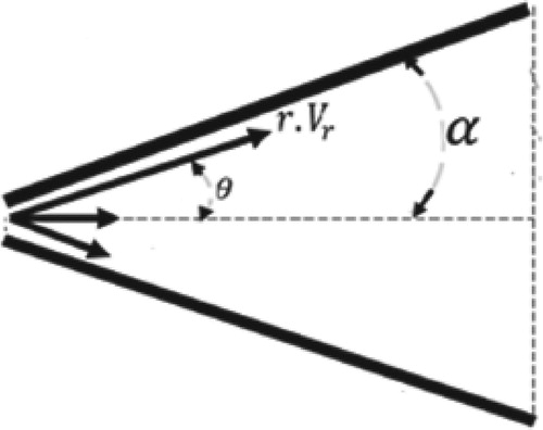
In vector form, the continuity and Navier-Stokes equations for Jeffery-Hamel flow are expressed as: (1) $\mathrm{\nabla }.\overrightarrow{V}=0$(1) (2) $\rho [(\overrightarrow{V}\overrightarrow{\mathrm{\nabla }})\overrightarrow{V}]=-\mathrm{\nabla }P+\mu .\mathrm{\Delta }\overrightarrow{V}$(2)

The Navier-Stokes equations can be provided as follows for cylindrical coordinates (r,θ, z): (3) $\begin{array}{rl}\frac{\rho }{r}.\frac{\mathrm{\partial }}{\mathrm{\partial }r}(r{V}_r)& =0\end{array}$(3) (4) $\begin{array}{rl}{V}_r.\frac{\mathrm{\partial }{V}_r}{\mathrm{\partial }r}& =-\frac{1}{\rho }.\frac{\mathrm{\partial }P}{\mathrm{\partial }r}+\nu .\\ & \times \left[\frac{{\mathrm{\partial }}^2{V}_r}{\mathrm{\partial }{r}^2}+\frac{1}{r}.\frac{\mathrm{\partial }{V}_r}{\mathrm{\partial }r}+\frac{1}{r^2}.\frac{{\mathrm{\partial }}^2{V}_r}{\mathrm{\partial }{\theta }^2}-\frac{V_r}{r^2}\right]\end{array}$(4) (5) $\begin{array}{rl}& -\frac{1}{\rho .r}.\frac{\mathrm{\partial }P}{\mathrm{\partial }\theta }+\frac{2.\nu }{r^2}.\frac{\mathrm{\partial }{V}_r}{\mathrm{\partial }\theta }=0\end{array}$(5) where: $V_r$: radial velocity; $\rho$: density; $\nu$: kinematic viscosity; P: fluid pressure.

In accordance with Equation (3), the quantities $(r.V_r)$ which are mainly dependant on $\theta$ can be provided below: (6) $r.V_r=f(\theta )$(6) It is well known that the net volume flux into the channel from the source at the origin is given as: (7) $Q={\int }_{-\alpha }^{+\alpha }r.V_{r}d\theta$(7)

Noted that any constant section, $r=cte$, is traveled by the same quantity $Q$.

For the studied Jeffery–Hamel flow, fluids can radially move outwards (i.e. in the diverging channel, $Q>0$) or inwards (i.e. in converging channel, $Q<0$). Also, it is well established that the maximal fluid velocity is undoubtedly provided at $\theta =0$. In fact, we obtain: (8) $r.V_{\text{max}}=f(0)$(8)

Consequently, $f(0)\ge f(\theta )$ in the range $-\alpha \le \theta \le +\alpha$.

Now introducing the dimensionless parameters (9) $F(\eta )=\frac{r.V_r}{r.V_{\text{max}}}=\frac{f(\theta )}{f_{\text{max}}},$(9) where: $\eta =\theta /\alpha$ with: $-1\le \eta \le +1$

Considering the kinematic fluid viscosity, $\nu$, the dimensionless quantities of the net volume flux (Equation (7)) may be expressed as follows: (10) $\frac{Q}{\nu }=R_e.{\int }_{-1}^{+1}F(\eta )d\eta$(10)

Where the Reynolds number can be introduced like: (11) $\begin{array}{rl}{R}_e& =\frac{r{V}_{\text{max}}\alpha }{\nu }=\frac{f_{\text{max}}.\alpha }{\nu }\\ & \times \{\begin{array}{l}{V}_{\text{max}}>0,\alpha >0\text{Divergent}\text{channel}\\ V_{\text{max}}<0,\alpha <0\text{Convergent}\text{channel}\end{array}\end{array}$(11) f_max expresses the velocity at the channel’s centerline, and, $\alpha$ indicates the channel half-angle. It is also worth noting that $(\alpha .r)$ measures the width of the channel.

By removing the pressure terms in Equations (4) and (5), it can be obtained: (12) $F^{\mathrm{\prime }\mathrm{\prime }\mathrm{\prime }}+2R_e\alpha F{F}^{\mathrm{\prime }}+4{\alpha }^2{F}^{\mathrm{\prime }}=0$(12) The boundary conditions associated with the Jeffery-Hamel flow in terms of $F(\eta )$ can be stated like: (13) $F(\eta )=1,F^{\mathrm{\prime }}(\eta )=0,$(13) at the centerline of channel (14) $F(\pm \eta )=0,$(14)

at the body of channelAccording to Batchelor [40], the Reynolds number based on the center-plane fluid velocity $V_{\text{max}}$, gives a direct measure of the flow intensity compared to the Reynolds number based on the flux: (15) $R=\frac{Q}{2\nu }=\frac{1}{2}\frac{Q}{\nu }=\frac{1}{2}{R}_e{\int }_{-1}^{+1}F(\eta )d\eta$(15)

2.2. Heat transferin Jeffery–Hamel flow

In the previous section, the governing Equations (3)–(5) mainly serve to achieve the hydrodynamical solution of the investigated flow inside convergent-divergent channels. For the aim of obtaining the thermal distribution in Jeffery-Hamel flow, we introduce the solution of the hydrodynamical part into the energy equation. In fact, the energy equationis given as: (16) $\rho .c_p(\overrightarrow{V}\overrightarrow{\mathrm{\nabla }})T=\varphi +K.{\mathrm{\nabla }}^{2}T$(16) where $K$ and $c_p$ indicate thermal conductivity and the specific heat at constant pressure, respectively.

Additionally, $\varphi$ expresses the viscous dissipation term which is provided below: (17) $\varphi =\mu \cdot [2{\epsilon }_{rr}^2+2{\epsilon }_{\theta \theta }^2+{\epsilon }_{r\theta }^2]$(17) The components of the strain tensor can be determined by: (18) $\{\begin{array}{l}{\epsilon }_{rr}=\frac{\mathrm{\partial }{V}_r}{\mathrm{\partial }r}\\ {\epsilon }_{\theta \theta }=\frac{1}{r}.\frac{\mathrm{\partial }{V}_{\theta }}{\mathrm{\partial }\theta }+\frac{V_r}{r}\\ {\epsilon }_{r\theta }=\frac{1}{r}.\frac{\mathrm{\partial }{V}_r}{\mathrm{\partial }\theta }+\frac{\mathrm{\partial }{V}_{\theta }}{\mathrm{\partial }r}-\frac{V_{\theta }}{r}\end{array}$(18) By taking into account the following transformations: (19) $T-T_{\mathrm{\infty }}=\frac{G(\theta )}{r^2}$(19)

In which $T_{\mathrm{\infty }}$ indicates the ambient temperature. The partial differential Equation (16) describing the thermal distribution in Jeffery–Hamel flow is lowered to an ODE after simplification: (20) $G^{\mathrm{\prime }\mathrm{\prime }}(\theta )+4G(\theta )+\frac{2f(\theta )}{d}G(\theta )=-\frac{\nu }{a{c}_p}(4f^2(\theta )+{f^{\mathrm{\prime }}}^2(\theta ))$(20) Where: $d=(K/\rho c_p)$ is the thermal diffusivity and, upon introducing the transformation (9) with the following quantities: (21) $\{\begin{array}{l}=\frac{\theta }{\alpha }\\ G^{\mathrm{\prime }}(\theta )=\frac{1}{\alpha }{G}^{\mathrm{\prime }}(\eta )\\ G^{\mathrm{\prime }\mathrm{\prime }}(\theta )=\frac{1}{{\alpha }^2}{G}^{\mathrm{\prime }\mathrm{\prime }}(\eta )\end{array}$(21) further reduction gives the dimensionless thermal distribution: (22) $\begin{array}{rl}& G^{\mathrm{\prime }\mathrm{\prime }}(\eta )+4{\alpha }^{2}G(\eta )+2R_e\alpha P_{r}FG(\eta )\\ & +P_r.X_r(4{\alpha }^2{F}^2+F^{{}^{\mathrm{\prime }}2})=0\end{array}$(22)

In which Re and Pr expressthe Re number given by (11) and Prandtl number ($P_r=(\nu /d)=(\mu .C_p/K)$), respectively.

The X_r term in Equation (22) can be determined below: (23) $\begin{array}{rl}{X}_r& =\frac{R_e^2.{\nu }^2}{{\alpha }^2.C_p}\end{array}$(23) The function $G(\eta )$ represents the dimensionless thermal distribution.

In terms of $G(\eta )$, the boundary conditions of heat transfer problem are given as: (24) $G^{\mathrm{\prime }}(0)=0,$(24) at the centerline of channel (25) $G(\pm \eta )=0,$(25) at the body of channel

3. Application of Adomian decomposition method to the Jeffery–Hamel problem

In this study, the set of nonlinear differential Equations (12) and (22) under the defined boundary conditions (13), (14), (24) and (25) were solved analytically utilizing the Adomian decomposition method.

It is worth noting that for solving the energy equation which governs the heat transfer in Jeffery-Hamel flow, it is necessary as a first step to solve the hydrodynamical part of the studied flow.

4.1. Hydrodynamical problem

According to the Adomian algorithm, Equation (12) can be written as: (26) $LF=-2R_e\alpha F{F}^{\mathrm{\prime }}-4{\alpha }^2{F}^{\mathrm{\prime }}$(26) In whichL is the differential operator that can be determined: $L=(d^3/d{\eta }^3)$.

The inverse of the operator $L$ is indicatedby $L^{-1}$. It is provided below: (27) $L^{-1}={\int }_0^{\eta }{\int }_0^{\eta }{\int }_0^{\eta }(\bullet )d\eta d\eta d\eta$(27)

By considering Equations (27), (26), and the boundary conditions (13) and (14), it can be obtained: (28) $F(\eta )=F(0)+F^{\mathrm{\prime }}(0)\eta +F^{\mathrm{\prime }\mathrm{\prime }}(0)\frac{{\eta }^2}{2}+L^{-1}(Nu)$(28) where: (29) $Nu=-2R_e\alpha F{F}^{\mathrm{\prime }}-4{\alpha }^2{F}^{\mathrm{\prime }}$(29)

Now, using boundary conditions (13), (14), and $F^{\mathrm{\prime }\mathrm{\prime }}(0)=a$, the following can be obtained: (30) $\begin{array}{r}F(\eta )=\sum _{n=0}^{\mathrm{\infty }}{F}_n=F_0+L^{-1}(Nu)\end{array}$(30)

where: (31) $F_0=1+a\frac{{\eta }^2}{2}$(31)

The first few terms of Adomian polynomials can beobtained with the use of the Adomian decomposition algorithm (Adomian & Adomian, 1994). In fact, we get: (32) $A_0=-2a\text{Re}\alpha \eta -4a{\alpha }^2\eta -a^2\text{Re}\alpha {\eta }^3$(32) (33) $\begin{array}{rl}{A}_1& =\frac{2}{3}a\text{R}{\text{e}}^2{\alpha }^2{\eta }^3+\frac{8}{3}a\text{Re}{\alpha }^3{\eta }^3+\frac{8}{3}a{\alpha }^4{\eta }^3\\ & +\frac{3}{5}{a}^2\text{R}{\text{e}}^2{\alpha }^2{\eta }^5+\frac{6}{5}{a}^2\text{Re}{\alpha }^3{\eta }^5+\frac{1}{15}{a}^3\text{R}{\text{e}}^2{\alpha }^2{\eta }^7\end{array}$(33) (34) $\begin{array}{rl}{A}_2& =\frac{1}{15}a\text{R}{\text{e}}^3{\alpha }^3{\eta }^5+\frac{2}{5}a\text{R}{\text{e}}^2{\alpha }^4{\eta }^5+\frac{4}{5}a\text{Re}{\alpha }^5{\eta }^5\\ & +\frac{8}{15}a{\alpha }^6{\eta }^5+\frac{11}{630}{a}^2\text{R}{\text{e}}^3{\alpha }^3{\eta }^7\\ & +\frac{22}{315}{a}^2\text{R}{\text{e}}^2{\alpha }^4{\eta }^7+\frac{22}{315}{a}^2\text{Re}{\alpha }^5{\eta }^7\\ & +\frac{11a^3\text{R}{\text{e}}^3{\alpha }^3{\eta }^9}{1890}+\frac{11}{945}{a}^3\text{R}{\text{e}}^2{\alpha }^4{\eta }^9\\ & +\frac{a^4\text{R}{\text{e}}^3{\alpha }^3{\eta }^{11}}{3600}\end{array}$(34)

On the other hand, by using Adomian decomposition algorithm (Adomian & Adomian, 1994), the first few components of the solution are: (35) $F_1=-\frac{1}{12}a\text{Re}\alpha {\eta }^4-\frac{1}{6}a{\alpha }^2{\eta }^4-\frac{1}{120}{a}^2\text{Re}\alpha {\eta }^6$(35) (36) $\begin{array}{rl}{F}_2& =-\frac{1}{180}a\text{R}{\text{e}}^2{\alpha }^2{\eta }^6-\frac{1}{45}a\text{Re}{\alpha }^3{\eta }^6-\frac{1}{45}a{\alpha }^4{\eta }^6\\ & -\frac{1}{560}{a}^2\text{R}{\text{e}}^2{\alpha }^2{\eta }^8-\frac{1}{280}{a}^2\text{Re}{\alpha }^3{\eta }^8-\frac{a^3\text{R}{\text{e}}^2{\alpha }^2{\eta }^{10}}{10800}\end{array}$(36) (37) $\begin{array}{rl}{F}_3& =-\frac{a\text{R}{\text{e}}^3{\alpha }^3{\eta }^8}{5040}-\frac{1}{840}a\text{R}{\text{e}}^2{\alpha }^4{\eta }^8-\frac{1}{420}a\text{Re}{\alpha }^5{\eta }^8\\ & -\frac{1}{630}a{\alpha }^6{\eta }^8-\frac{11a^2\text{R}{\text{e}}^3{\alpha }^3{\eta }^{10}}{453600}-\frac{11a^2\text{R}{\text{e}}^2{\alpha }^4{\eta }^{10}}{113400}\\ & -\frac{11a^2\text{Re}{\alpha }^5{\eta }^{10}}{113400}-\frac{a^3\text{R}{\text{e}}^3{\alpha }^3{\eta }^{12}}{226800}-\frac{a^3\text{R}{\text{e}}^2{\alpha }^4{\eta }^{12}}{113400}\\ & -\frac{a^4\text{R}{\text{e}}^3{\alpha }^3{\eta }^{14}}{7862400}\end{array}$(37)

Ultimately, the estimated answer for the hydrodynamical problem can be provided: (38) $F(\eta )=F_0+F_1+F_2+F_3+\dots +F_n$(38)

With using Equations (38) and (14), the constant a could be determined.

4.2. Heat transfer problem

With using ADM on the heat transfer problem, we obtain: (39) $LG+P_r.X_r(4{\alpha }^2{F}^2+F^{{}^{\mathrm{\prime }}2})=-4{\alpha }^{2}G-2R_e\alpha P_{r}FG$(39) In whichL can be provided as $L=(d^2/d{\eta }^2)$.

Additionally, the inverse of $L$ can be provided like: $L^{-1}={\int }_0^{\eta }{\int }_0^{\eta }.d\eta d\eta (40)$

The application of Equation (40) on Equation (39) yields: (41) $G(\eta )=G(0)+L^{-1}(Ng)$(41) where: (42) $Ng=-4{\alpha }^{2}G-2R_e\alpha P_{r}FG$(42)

In contrast, if the boundary conditions (24)–(25), and $G(0)=b$ are applied, the following could be achieved: (43) $\begin{array}{rl}G(\eta )& =\sum _{n=0}^{\mathrm{\infty }}{G}_n=G_0+L^{-1}(Ng)\end{array}$(43)

where (44) $G_0=b-\frac{1}{2}{F}^{\mathrm{\prime }2}\text{Pr Xr }{\eta }^2-2F^2\text{ Pr Xr}{\alpha }^2{\eta }^2$(44)

For heat transfer problem, with using ADM (Adomian & Adomian, 1994), the terms of solution and the Adomian polynomials can be provided: (45) $\begin{array}{rl}{B}_0& =-2bF\text{PrRe}\alpha -4b{\alpha }^2-4c{\alpha }^2\eta +F^{\mathrm{\prime }2}F\text{P}{\text{r}}^2\text{ReXr}\alpha {\eta }^2\\ & +2F^{\mathrm{\prime }2}\text{PrXr}{\alpha }^2{\eta }^2\\ & +4F^3\text{P}{\text{r}}^2\text{ReXr}{\alpha }^3{\eta }^2+8F^2\text{ PrXr}{\alpha }^4{\eta }^2\end{array}$(45) (46) $\begin{array}{rl}{G}_1& =-bF\text{PrRe}\alpha {\eta }^2-2b{\alpha }^2{\eta }^2+\frac{1}{12}{F}^{\mathrm{\prime }2}F\text{P}{\text{r}}^2\text{ReXr}\alpha {\eta }^4\\ & +\frac{1}{6}{F}^{\mathrm{\prime }2}\text{PrXr}{\alpha }^2{\eta }^4+\frac{1}{3}F{F}^2\text{P}{\text{r}}^2\text{ReXr}{\alpha }^3{\eta }^4\\ & +\frac{2}{3}{F}^2\text{Pr Xr}{\alpha }^4{\eta }^4\end{array}$(46) (47) $\begin{array}{rl}{B}_1& =2b{F}^2\text{P}{\text{r}}^2\text{R}{\text{e}}^2{\alpha }^2{\eta }^2+8bF\text{PrRe}{\alpha }^3{\eta }^2+8b{\alpha }^4{\eta }^2\\ & -\frac{1}{6}{F^{\mathrm{\prime }}}^2{F}^2\text{P}{\text{r}}^3\text{R}{\text{e}}^2\text{Xr}{\alpha }^2{\eta }^4\\ & -\frac{2}{3}{F^{\mathrm{\prime }}}^{2}F\text{P}{\text{r}}^2\text{ReXr}{\alpha }^3{\eta }^4-\frac{2}{3}{F^{\mathrm{\prime }}}^2\text{PrXr}{\alpha }^4{\eta }^4\\ & -\frac{2}{3}{F}^4\text{P}{\text{r}}^3\text{R}{\text{e}}^2\text{Xr}{\alpha }^4{\eta }^4-\frac{8}{3}{F}^3\text{P}{\text{r}}^2\text{ReXr}{\alpha }^5{\eta }^4\\ & -\frac{8}{3}{F}^2\text{PrXr}{\alpha }^6{\eta }^4\end{array}$(47) (48) $\begin{array}{rl}{G}_2& =\frac{1}{6}b{F}^2\text{P}{\text{r}}^2\text{R}{\text{e}}^2{\alpha }^2{\eta }^4+\frac{2}{3}bF\text{PrRe}{\alpha }^3{\eta }^4+\frac{2}{3}b{\alpha }^4{\eta }^4\\ & -\frac{1}{180}{F^{\mathrm{\prime }}}^2{F}^2\text{P}{\text{r}}^3\text{R}{\text{e}}^2\text{Xr}{\alpha }^2{\eta }^6\\ & -\frac{1}{45}{F^{\mathrm{\prime }}}^{2}F\text{P}{\text{r}}^2\text{ReXr}{\alpha }^3{\eta }^6-\frac{1}{45}{F^{\mathrm{\prime }}}^2\text{PrXr}{\alpha }^4{\eta }^6\\ & -\frac{1}{45}{F}^4\text{P}{\text{r}}^3\text{R}{\text{e}}^2\text{Xr}{\alpha }^4{\eta }^6-\frac{4}{45}{F}^3\text{P}{\text{r}}^2\text{ReXr}{\alpha }^5{\eta }^6\\ & -\frac{4}{45}{F}^2\text{PrXr}{\alpha }^6{\eta }^6\end{array}$(48) (49) $\begin{array}{rl}{B}_2=& -\frac{1}{3}b{F}^3\text{P}{\text{r}}^3\text{R}{\text{e}}^3{\alpha }^3{\eta }^4-2b{F}^2\text{P}{\text{r}}^2\text{R}{\text{e}}^2{\alpha }^4{\eta }^4\\ & -4bF\text{PrRe}{\alpha }^5{\eta }^4-\frac{8}{3}b{\alpha }^6{\eta }^4\\ & +\frac{1}{90}{F^{\mathrm{\prime }}}^2{F}^3\text{P}{\text{r}}^4\text{R}{\text{e}}^3\text{Xr}{\alpha }^3{\eta }^6+\frac{1}{15}{F^{\mathrm{\prime }}}^2{F}^2\text{P}{\text{r}}^3\text{R}{\text{e}}^2\\ & \times \text{Xr}{\alpha }^4{\eta }^6+\frac{2}{15}{F^{\mathrm{\prime }}}^{2}F\text{P}{\text{r}}^2\text{ReXr}{\alpha }^5{\eta }^6\\ & +\frac{2}{45}{F}^5\text{P}{\text{r}}^4\text{R}{\text{e}}^3\text{Xr}{\alpha }^5{\eta }^6+\frac{4}{45}{F^{\mathrm{\prime }}}^2\text{PrXr}{\alpha }^6{\eta }^6\\ & +\frac{4}{15}{F}^4\text{P}{\text{r}}^3\text{R}{\text{e}}^2\text{Xr}{\alpha }^6{\eta }^6+\frac{8}{15}{F}^3\text{P}{\text{r}}^2\text{ReXr}{\alpha }^7{\eta }^6\\ & +\frac{16}{45}{F}^2\text{PrXr}{\alpha }^8{\eta }^6\end{array}$(49) (50) $\begin{array}{rl}{G}_3& =-\frac{1}{90}b{F}^3\text{P}{\text{r}}^3\text{R}{\text{e}}^3{\alpha }^3{\eta }^6-\frac{1}{15}b{F}^2\text{P}{\text{r}}^2\text{R}{\text{e}}^2{\alpha }^4{\eta }^6\\ & -\frac{2}{15}bF\text{PrRe}{\alpha }^5{\eta }^6-\frac{4}{45}b{\alpha }^6{\eta }^6\\ & +\frac{1}{5040}{F^{\mathrm{\prime }}}^2{F}^3\text{P}{\text{r}}^4\text{R}{\text{e}}^3\text{Xr}{\alpha }^3{\eta }^8\\ & +\frac{1}{840}{F^{\mathrm{\prime }}}^2{F}^2\text{P}{\text{r}}^3\text{R}{\text{e}}^2\text{Xr}{\alpha }^4{\eta }^8\\ & +\frac{1}{420}{F^{\mathrm{\prime }}}^{2}F\text{P}{\text{r}}^2\text{ReXr}{\alpha }^5{\eta }^8\\ & +\frac{1}{1260}{F}^5\text{P}{\text{r}}^4\text{R}{\text{e}}^3\text{Xr}{\alpha }^5{\eta }^8+\frac{1}{630}{F^{\mathrm{\prime }}}^2\text{PrXr}{\alpha }^6{\eta }^8\\ & +\frac{1}{210}{F}^4\text{P}{\text{r}}^3\text{R}{\text{e}}^2\text{Xr}{\alpha }^6{\eta }^8\\ & +\frac{1}{105}{F}^3\text{P}{\text{r}}^2\text{ReXr}{\alpha }^7{\eta }^8+\frac{2}{315}{F}^2\text{PrXr}{\alpha }^8{\eta }^8\end{array}$(50) (51) $\begin{array}{rl}{B}_3& =\frac{1}{2520}b{F}^4\text{P}{\text{r}}^4\text{R}{\text{e}}^4{\alpha }^4{\eta }^8+\frac{1}{315}b{F}^3\text{P}{\text{r}}^3\text{R}{\text{e}}^3{\alpha }^5{\eta }^8\\ & +\frac{1}{105}b{F}^2\text{P}{\text{r}}^2\text{R}{\text{e}}^2{\alpha }^6{\eta }^8\\ & +\frac{4}{315}bF\text{PrRe}{\alpha }^7{\eta }^8+\frac{2}{315}b{\alpha }^8{\eta }^8\\ & -\frac{1}{226800}{F^{\mathrm{\prime }}}^2{F}^4\text{P}{\text{r}}^5\text{R}{\text{e}}^4\text{Xr}{\alpha }^4{\eta }^{10}\\ & -\frac{1}{28350}{F^{\mathrm{\prime }}}^2{F}^3\text{P}{\text{r}}^4\text{R}{\text{e}}^3\text{Xr}{\alpha }^5{\eta }^{10}\\ & -\frac{1}{9450}{F^{\mathrm{\prime }}}^2{F}^2\text{P}{\text{r}}^3\text{R}{\text{e}}^2\text{Xr}{\alpha }^6{\eta }^{10}\\ & -\frac{1}{56700}{F}^6\text{P}{\text{r}}^5\text{R}{\text{e}}^4\text{Xr}{\alpha }^6{\eta }^{10}\\ & -\frac{2}{14175}{F^{\mathrm{\prime }}}^{2}F\text{P}{\text{r}}^2\text{ReXr}{\alpha }^7{\eta }^{10}\\ & -\frac{2}{14175}{F}^5\text{P}{\text{r}}^4\text{R}{\text{e}}^3\text{Xr}{\alpha }^7{\eta }^{10}\\ & -\frac{1}{14175}{F^{\mathrm{\prime }}}^2\text{PrXr}{\alpha }^8{\eta }^{10}\\ & -\frac{2}{4725}{F}^4\text{P}{\text{r}}^3\text{R}{\text{e}}^2\text{Xr}{\alpha }^8{\eta }^{10}\\ & -\frac{8}{14175}{F}^3\text{P}{\text{r}}^2\text{ReXr}{\alpha }^9{\eta }^{10}\\ & -\frac{4}{14175}{F}^2\text{PrXr}{\alpha }^{10}{\eta }^{10}\end{array}$(51) (52) $\begin{array}{rl}{G}_4& =\frac{1}{2520}b{F}^4\text{P}{\text{r}}^4\text{R}{\text{e}}^4{\alpha }^4{\eta }^8+\frac{1}{315}b{F}^3\text{P}{\text{r}}^3\text{R}{\text{e}}^3{\alpha }^5{\eta }^8\\ & +\frac{1}{105}b{F}^2\text{P}{\text{r}}^2\text{R}{\text{e}}^2{\alpha }^6{\eta }^8+\frac{4}{315}bF\text{PrRe}{\alpha }^7{\eta }^8\\ & +\frac{2}{315}b{\alpha }^8{\eta }^8-\frac{1}{226800}{F^{\mathrm{\prime }}}^2{F}^4\text{P}{\text{r}}^5\text{R}{\text{e}}^4\text{Xr}{\alpha }^4{\eta }^{10}\\ & -\frac{1}{28350}{F^{\mathrm{\prime }}}^2{F}^3\text{P}{\text{r}}^4\text{R}{\text{e}}^3\text{Xr}{\alpha }^5{\eta }^{10}\\ & -\frac{1}{9450}{F^{\mathrm{\prime }}}^2{F}^2\text{P}{\text{r}}^3\text{R}{\text{e}}^2\text{Xr}{\alpha }^6{\eta }^{10}\\ & -\frac{1}{56700}{F}^6\text{P}{\text{r}}^5\text{R}{\text{e}}^4\text{Xr}{\alpha }^6{\eta }^{10}\\ & -\frac{2}{14175}{F^{\mathrm{\prime }}}^{2}F\text{P}{\text{r}}^2\text{ReXr}{\alpha }^7{\eta }^{10}\\ & -\frac{2}{14175}{F}^5\text{P}{\text{r}}^4\text{R}{\text{e}}^3\text{Xr}{\alpha }^7{\eta }^{10}\\ & -\frac{1}{14175}{F^{\mathrm{\prime }}}^2\text{PrXr}{\alpha }^8{\eta }^{10}\\ & -\frac{2}{4725}{F}^4\text{P}{\text{r}}^3\text{R}{\text{e}}^2\text{Xr}{\alpha }^8{\eta }^{10}-\frac{8}{14175}{F}^3\text{P}{\text{r}}^2\text{ReXr}{\alpha }^9{\eta }^{10}\\ & -\frac{4}{14175}{F}^2\text{PrXr}{\alpha }^{10}{\eta }^{10}\end{array}$(52)

Ultimately, the estimated answer of the heat transfer model in Jeffery-Hamel flow can be provided as: (53) $G(\eta )=G_0+G_1+G_2+G_3+\dots +G_n$(53)

Equations (53) and (25) can be employed to calculate the constant of b.

5. Results and Discussions

A parametric investigation has been performed for showing the effect of Reynolds and Prandtl numbers on the behavior of heat transfer and fluid velocity in Jeffery-Hamel flow between non-parallel plane walls. It is worth stating that, for the heat transfer problem, four ranges of fluids flow including steam, liquid metal, air, and water have been considered. Table 1 states the thermophysical properties of used fluids in this study.

Table 1. Thermophysical properties of the studied fluids.

Properties	LiquidMetal	Air	Steam	Water
Kinematic viscosity, ν (m^2/s)	38758.753 × 10^−11	5.850 × 10^−5	0.372 × 10^−5	1.007 × 10^−6
Prandtl number, Pr	0.01174	0.6843	1.11	7
Heat capacity, Cp(J/Kg.°K)	913	1063	2305	4178

In this research, both analytical and numerical solutions were computed. In fact, an analytical solution is gained using the Adomian Decomposition Method (ADM); however, the numerical solution is achieved by using Runge–Kutta-Fehlberg based on the shooting approach.

Figures 2–12 show thermal distributions and the velocity profiles in convergent-divergent channels associated with the obtained analytical and numerical values for the objective of highlighting the significance of the studied flow.

Figure 2. Effects of Reynolds number on fluid velocity profiles inside convergent channel.

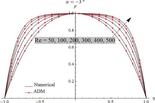
Figure 3. Effects of Reynolds number on fluid velocity inside divergent channel.

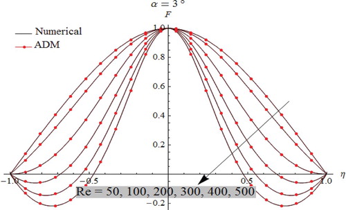
Figure 4. Effect of channel-half angle α on fluid velocity inside convergent channel.

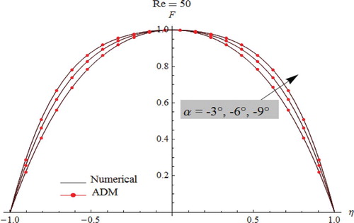
Figure 5. Effect of channel-half angle α on fluid velocity inside divergent channel.

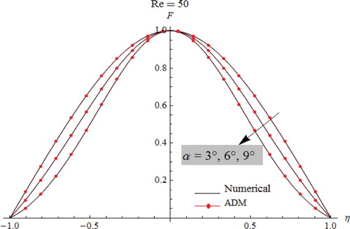
Figure 6. Thermal profiles under the effect of Reynolds number in converging channel for steam flow.

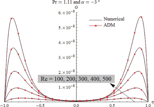
Figure 7. Thermal profiles under the effect of Reynolds number in converging channel for air flow.

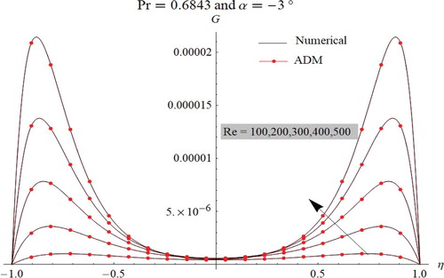
Figure 8. Thermal profiles under the effect of Reynolds number in converging channel for metal liquid flow.

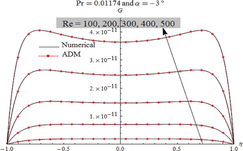
Figure 9. Thermal profiles under the effect of Reynolds number in diverging channel for steam flow.

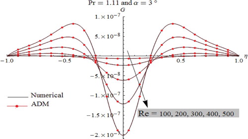
Figure 10. Thermal profiles under the effect of Reynolds number in diverging channel for air flow.

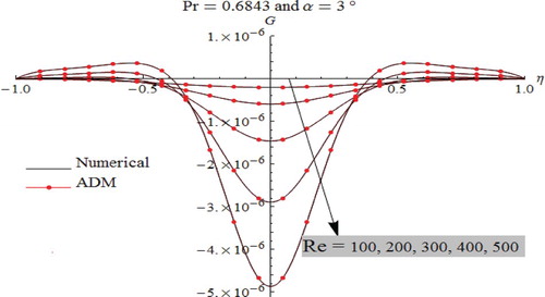
Figure 11. Thermal profiles under the effect of Reynolds number in diverging channel for metal liquid flow.

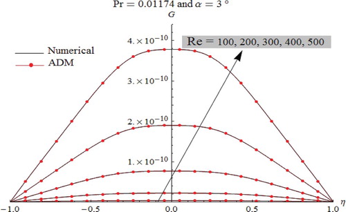
Figure 12. Thermal profiles under the effect of Reynolds number in diverging channel for water flow.

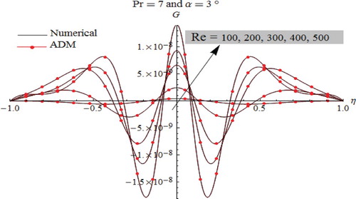
Figure 2 illustrates the influences of Re number on the fluid velocity of the convergent flow.

In fact, a flatter profile at the center of the channel with great gradients close to the walls can be obtained by augmenting Re number. As a consequence, the thicknesses of the boundary layer decreases. For convergent flow cases, it is well clear that the backflow is entirely precluded. Figure 3 illustrates the influence of Reynolds number on divergent flow which is to concentrate the volume flux at the center of channels with smaller gradients near the walls. For purely divergent channels, results obtained reveal that the flow reversal is highly favored. Figures 4 and 5 illustrate the impact of the channel-half angle $\alpha$ on the fluid velocity. Here, the velocity behavior is expected to be identical, which occurred in the case of Re number influence. As shown in Figure 4 for the case of convergent flow, we observe that the backflow phenomenon is precluded, but this phenomenon is highly observed inside divergent channels as depicted in Figure 5.

Heat transfer behavior in convergent-divergentchannels is displayed in Figures 6–12. In the convergent channel, for the case of steam and Air flows as shown in Figures 6 and 7, we notice that the minimum temperature is observed through the channel axis, while the maximum temperature occurs in the vicinity of the plates. Furthermore, as presented in Figure 8, for liquid metal flow in convergent channels, the thermal profiles show an identical behavior on the entire channel.

As displayed in Figures 9–11, the characteristic behavior of fluid temperature in the diverging channel is fairly various in which the oscillations are worthy. The presence of oscillations depends on the nature of the studied fluids. Here, it is highly noted that the apparition of oscillations is mainly related to the Prandtl number. In fact, we notice the total absence of oscillations for liquid metal flow (Figure 11), while their presence is clearly noticed in the case of Air and Steam flows (Figures 9 and 10).

According to the obtained results for both convergent-divergent channels, it can be concluded which the steam (Pr=1.11) and air (Pr=0.6843) have vicious behavior. In fact, with increasing Reynolds number Re it appears that the heat dissipation is very higher near the plates than that observed along the channel axis. Also, it is clearly noticed that the heat dissipation is higher for air flow when compared to that occurred in regards to the steam flow. In contrast, the liquid metal (Pr=0.01174) is considered as a conductor fluid for both convergent-divergent channels. In such a case, the heat dissipation for liquid metal flow is lower when compared to that occurred for the other ranges of fluids.

As presented in Figure 12 in the case of the divergent channel, it is clearly shown for higher Prandtl value (Pr=7; water flow case) that the thermal behavior becomes quite different. In fact, thermal profiles contain a large number of oscillations with several minima and maxima.

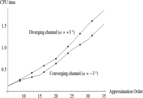
Figure 13 shows the behavior of CPU time versus channel-half angle (α) and the order of approximation. In fact, obtained results reveal that the CPU time is very short (i.e. few seconds), thus justifying the fast convergence of the adopted ADM algorithm.

Figure 13. CPU time of ADM vs approximation order in converging/diverging channels.

For all simulations cases, as displayed in Figures 2–12, comparison between ADM results and numerical one used as a guide reveals that the outcomes are identical to each other, which justify and confirm that both the Adomian Decomposition method and numerical Runge–Kutta–Fehlberg are valid, applicable, and have great precision.

As depicted in Table 2, for velocity distribution through convergent/divergent channels when Re=43 and α=3°, the error between ADM and numerical data is introduced as: $|F_{\text{Numerical}}-F_{\text{ADM}}|$

Table 2. Comparison between Numerical and ADM solutions for velocity distribution through convergent/divergent channels when Re = 43.

	Divergingchannel (α =+ 3°)			Convergingchannel(α= - 3°)
η	FNumerical	FADM	|FNumerical - FADM |	FNumerical	FADM	|FNumerical - FADM |
0.00	1.000000000000	1.000000000000	0.00000000	1.00000000000	1.00000000000	0.00000000
0.25	0.9176760582677312	0.9176760639989867	5.73×10^−9	0.952601226585409	0.952601233559707	6.97×10^−9
0.50	0.6916137868663034	0.6916137895560733	2.68×10^−9	0.7974632865663513	0.7974632807505999	5.81×10^−9
0.75	0.370363266835419	0.37036327154516463	4.70×10^−9	0.497128632405185	0.4971286000590072	3.23×10^−8
1.00	0.000000000000	0.000000000000	0.000000000	0.00000000000	0.0000000000	0.0000000

The numerical data of F''(0) for different values of Re and α=±5° are expressed in Table 3. From results obtained, as drawn in Tables 2 and 3, an appropriate agreement is monitored between ADM analytical solution, numerical RK4 solution, and available data in references (Abbasbandy & Shivanian, 2012; Kezzar et al., 2018).

Table 3. ADM analytical results for F''(0).

	Convergingchannel (α=−5°)			Divergingchannel (α=+5°)
Re	F''(0)(Abbasbandy & Shivanian, 2012)	F''(0) (Kezzar et al., 2018)	F''(0) [Presentstudy]	F''(0) (Abbasbandy & Shivanian, 2012)	F''(0) (Kezzar et al., 2018)	F''(0) [Presentstudy]
10	−1.7845468	−1.7845469	−1.7845467711404606	−2.2519486	−2.2519485	−2.251948586722248
20	−1.5881535	−1.5881533	−1.5881534850176322	−2.5271922	−2.5271921	−2.527192251461816
30	−1.4136920	−1.4136921	−1.4136920839885079	−2.8326293	−2.8326295	−2.832629313353397
40	−1.2589939	−1.2589937	−1.2589939169568094	−3.1697121	−3.1697120	−3.169712202009959
50	−1.1219890	−1.1219891	−1.121989146674565	−3.5394156	−3.5394155	−3.539415629020588

On the other hand, Tables 4 and 6 illustrate the numerical data of thermal distributions in convergent-divergent channels (case of liquid metal, Air and Steam) once Reynolds number is equal to 50 and channel-half angle α=3°. In these tables, the error is introduced as Table 5: $\text{Error}=\left|\frac{G{(\eta )}_{\text{Num}}-G{(\eta )}_{\text{ADM}}}{G{(\eta )}_{\text{NUM}}}\right|$

Table 4. Comparison between ADM and Numerical results in convergent-divergent channels when Re=50 and α=3° (Thermal distribution in the case of liquid metal flow).

	Converging			Diverging
η	Numerical × 10^−10	ADM × 10^−10	Error	Numerical × 10^−10	ADM x10^−10	Error
0	5,884051	5,884084	0.00000560838	7,726855	7,726817	0.00000491791
0,2	5,880418	5,880451	0.00000561185	7,691383	7,691345	0.00000494059
0,4	5,798519	5,798552	0.00000569111	7,369621	7,369586	0.00000474923
0,6	5,366264	5,366292	0.00000521778	6,266984	6,266959	0.00000398916
0,8	3,911092	3,911106	0.00000357956	3,905974	3,905967	0.00000179213

Table 5. Comparison between ADM and Numerical results in convergent-divergent channels when Re=50 and α=3° (Thermal distribution in the case of Air flow).

	Converging			Diverging
η	Numerical × 10^−8	ADM × 10^−8	Error	Numerical × 10^−7	ADM × 10^−7	Error
0	1,267192	1,2672	0.0000063131	−2,251551	−2,251531	0.00000888277
0,2	1,352753	1,352762	0.0000066531	−2,094514	−2,094496	0.00000859388
0,4	1,574144	1,574154	0.00000635266	−1,673251	−1,673237	0.00000836695
0,6	1,780953	1,780962	0.00000505347	−1,107112	−1,107102	0.00000903251
0,8	1,561094	1,561098	0.00000256231	−0,5215149	−0,5215095	0.00000103545

Table 6. Comparison between ADM and Numerical results in convergent-divergent channels when Re=50 and α=3° (Thermal distribution in the case of Steam flow).

η	Converging			Diverging
η	Numerical × 10^−10	ADM × 10^−10	Error	Numerical × 10^−9	ADM × 10^−9	Error
0	4,509989	4,510017	0.00000620844	−3,053678	−3,053661	0.00000556706
0,2	5,010631	5,010664	0.000006586	−2,715585	−2,71557	0.00000552367
0,4	6,36858	6,368621	0.00000643786	−1,874873	−1,874862	0.00000586706
0,6	7,88654	7,886584	0.00000557913	−0,9252627	−0,9252555	0.00000778157
0,8	7,431525	7,431546	0.0000028258	−0,2338741	−0,2338685	0.00000239445

According to the results obtained, it should be stressed which a great match can be observed in both numerical and analytical data.

Finally, the values of constant $G(0)=b$ which represents the temperature at the level of channel’s center are gathered in Table 7. These values are calculated for all temperature curves (Figures 6–12).

Table 7. Values of dimensionless temperature at the channel centerline:$G(0)=b$.

Re	Convergingchannel(α = − 3°)			Divergingchannel(α = ± 3°)
	Liquid Metal	Air	Steam	Liquid Metal	Air	Steam	Water
100	1.96×10^−12	4.33×10^−7	7.28×10^−10	3.42×10^−12	−3.586×10^−6	−6.26×10^−9	4.26×10^−10
200	7.04×10^−12	5.98×10^−7	7.83×10^−10	2.20×10^−11	−0.00001049	−2.3×10^−8	2.45×10^−9
300	1.47×10^−11	5.93×10^−7	6.4×10^−10	7.67×10^−11	−0.00002583	−6.14×10^−8	6.63×10^−9
400	2.46×10^−11	5.34×10^−7	5.07×10^−10	1.89×10^−10	−0.00005122	−1.21×10^−7	9.31×10^−9
500	3.63×10^−11	4.65×10^−7	4.07×10^−10	3.78×10^−10	−0.00008621	−2.01×10^−7	1.41×10^−8

6. Concluding Remarks

In this investigation, the steady 2D flows between non-parallel plane walls have been considered. The arising ODEs from mathematical modeling have been computed analytically and numerically. In fact, an analytical solution is gained via the Adomian Decomposition Method, while the numerical solution is computed with the help of Runge–Kutta-Fehlberg scheme based on shooting technique.

Some crucial findings can be enumerated as the fundamental conclusions of this research:

• A straighter profile at the channel’s center can be achieved by augmenting Reynolds number of the convergent flow; subsequently, it results in a reduction in the boundary layer thickness.

• In divergent flow, augmenting Re number leads to the concentration of the volume flux at the channel’s center. In such cases, the boundary layer thickness expands by augmenting Re number.

• Fluid velocity in the convergent channel is increased by a rise in the channel half-angle ($\alpha$), whereas a reverse behavior may occur in the divergent channel.

• The backflow phenomenon in divergent channels might happen for greater amounts of channel half-angle ($\alpha$) under the condition of a high adverse pressure gradient.

• Thermal distributions in the converging channel are similar in the case of Air and Steam flows, whereas the behavior is extensively distinct in the diverging channel in which the oscillations are notable.

• The oscillations number in divergent channels mainly depends on the nature of flowing fluid. In fact, an increase in Prandtl number results in raising the oscillations.

• The heat dissipation is lower for liquid metal flow compared to the heat dissipation observed for Air and Steam flows.

• Results obtained for dimensionless fluid velocity and thermal distribution illustrate a great match between ADM and numerical solution. Therefore, both numerical and analytical methods are valid, applicable, and have great precision.

Disclosure statement

No potential conflict of interest was reported by the author(s).

Correction Statement

This article has been republished with minor changes. These changes do not impact the academic content of the article.

References

- Abbasbandy, S. (2007). A numerical solution of Blasius equation by Adomian’s decomposition method and comparison with homotopy perturbation method. Chaos, Solitons and Fractals, 31(1), 257–260. https://doi.org/10.1016/j.chaos.2005.10.071
- Abbasbandy, S., & Shivanian, E. (2012). Exact analytical solution of the MHD Jeffery-Hamel flow problem. Meccanica, 47(6), 1379–1389. https://doi.org/10.1007/s11012-011-9520-3
- Adomian, G., & Adomian, G. (1994). On Modelling Physical Phenomena. In Solving Frontier problems of Physics: The Decomposition method (pp. 1–5). Springer. https://doi.org/10.1007/978-94-015-8289-6_1
- Alizadeh, E., Farhadi, M., Sedighi, K., Ebrahimi-Kebria, H. R., & Ghafourian, A. (2009). Solution of the Falkner-Skan equation for wedge by Adomian Decomposition method. Communications in Nonlinear Science and Numerical Simulation, 14(3), 724–733. https://doi.org/10.1016/j.cnsns.2007.11.002
- Alizadeh, E., Sedighi, K., Farhadi, M., & Ebrahimi-Kebria, H. R. (2009). Analytical approximate solution of the cooling problem by Adomian decomposition method. Communications in Nonlinear Science and Numerical Simulation, 14(2), 462–472. https://doi.org/10.1016/j.cnsns.2007.09.008
- Baghban, A., Sasanipour, J., Pourfayaz, F., Ahmadi, M. H., Kasaeian, A., Chamkha, A. J., Oztop, H. F., & Chau, K. (2019). Towards experimental and modeling study of heat transfer performance of water- SiO2 nanofluid in quadrangular cross-section channels. Engineering Applications of Computational Fluid Mechanics, 13(1), 453–469. https://doi.org/10.1080/19942060.2019.1599428
- Eagles, P. M. (1966). The stability of a family of Jeffery–Hamel solutions for divergent channel flow. Journal of Fluid Mechanics, 24(1), 191–207. https://doi.org/10.1017/S0022112066000582
- Gao, T., Zhu, J., Li, J., & Xia, Q. (2018). Numerical study of the influence of rib orientation on heat transfer enhancement in two-pass ribbed rectangular channel. Engineering Applications of Computational Fluid Mechanics, 12(1), 117–136. https://doi.org/10.1080/19942060.2017.1360210
- Gherieb, S., Kezzar, M., & Sari, M. R. (2020). Analytical and numerical solutions of heat and mass transfer of boundary layer flow in the presence of a transverse magnetic field. Heat Transfer, 49(3), 1129–1148. https://doi.org/10.1002/htj.21655
- Gholami, A., Bonakdari, H., Zaji, A. H., & Akhtari, A. A. (2015). Simulation of open channel bend characteristics using computational fluid dynamics and artificial neural networks. Engineering Applications of Computational Fluid Mechanics, 9(1), 355–369. https://doi.org/10.1080/19942060.2015.1033808
- Goldberg, U. C., Palaniswamy, S., Batten, P., & Gupta, V. (2010). Variable Turbulent Schmidt and Prandtl number modeling. Engineering Applications of Computational Fluid Mechanics, 4(4), 511–520. https://doi.org/10.1080/19942060.2010.11015337
- Hamadiche, M., Scott, J., & Jeandel, D. (1994). Temporal stability of Jeffery-Hamel flow. Journal of Fluid Mechanics, 268(6), 71–88. https://doi.org/10.1017/S0022112094001266
- He, J. H. (2003). Homotopy perturbation method: A new nonlinear analytical technique. Applied Mathematics and Computation, 135(1), 73–79. https://doi.org/10.1016/S0096-3003(01)00312-5
- He, J. H., & Wu, X. H. (2007). Variational iteration method: New development and applications. Computers and Mathematics with Applications, 54(7–8), 881–894. https://doi.org/10.1016/j.camwa.2006.12.083
- Jeffery, G. B. (1915). L. The two-dimensional steady motion of a viscous fluid. The London, Edinburgh, and Dublin Philosophical Magazine and Journal of Science, 29(172), 455–465. https://doi.org/10.1080/14786440408635327
- Kezzar, M., & Sari, M. R. (2017). Series solution of nanofluid flow and heat transfer between stretchable/shrinkable inclined walls. International Journal of Applied and Computational Mathematics, 3(3), 2231–2255. https://doi.org/10.1007/s40819-016-0238-8
- Kezzar, M., Sari, M. R., Bourenane, R., Rashidi, M. M., & Haiahem, A. (2018). Heat transfer in hydro-magnetic nano-fluid flow between non-parallel plates using DTM. Journal of Applied and Computational Mechanics, 4(4), 352–364. https://doi.org/10.22055/JACM.2018.24959.1221
- Khan, U., Adnan, Ahmed, N., & Mohyud-Din, S. T. (2017). Soret and Dufour effects on Jeffery-Hamel flow of second-grade fluid between convergent/divergent channel with stretchable walls. Results in Physics, 7, 361–372. https://doi.org/10.1016/j.rinp.2016.12.020
- Li, Z., Khan, I., Shafee, A., Tlili, I., & Asifa, T. (2018). Energy transfer of Jeffery–Hamel nanofluid flow between non-parallel walls using Maxwell–Garnetts (MG) and Brinkman models. Energy Reports, 4, 393–399. https://doi.org/10.1016/j.egyr.2018.05.003
- Liao, S. (2003). Beyond perturbation. In Beyond perturbation. Chapman and Hall/CRC. https://doi.org/10.1201/9780203491164
- Liao, S. J., & Cheung, K. F. (2003). Homotopy analysis of nonlinear progressive waves in deep water. Journal of Engineering Mathematics, 45(2), 105–116. https://doi.org/10.1023/A:1022189509293
- Mahmood, A., Md Basir, M., Ali, U., Mohd Kasihmuddin, M., & Mansor, M. (2019). Numerical solutions of heat transfer for magnetohydrodynamic Jeffery-Hamel flow using spectral homotopy analysis method. Processes, 7(9), 626. https://doi.org/10.3390/pr7090626
- Millsaps, K., & Pohlhausen, K. (1953). Thermal distributions in Jeffery-Hamel flows between nonparallel plane walls. Journal of the Aeronautical Sciences, 20(3), 187–196. https://doi.org/10.2514/8.2587
- Moradi, A., Alsaedi, A., & Hayat, T. (2013). Investigation of nanoparticles effect on the Jeffery-Hamel flow. Arabian Journal for Science and Engineering, 38(10), 2845–2853. https://doi.org/10.1007/s13369-012-0472-2
- Ramezanizadeh, M., Alhuyi Nazari, M., Ahmadi, M. H., & Chau, K. (2019). Experimental and numerical analysis of a nanofluidic thermosyphon heat exchanger. Engineering Applications of Computational Fluid Mechanics, 13(1), 40–47. https://doi.org/10.1080/19942060.2018.1518272
- RamReddy, C., Pradeepa, T., Venkata Rao, C., Surender, O., & Chitra, M. (2017). Analytical solution of mixed convection flow of a Newtonian fluid between vertical parallel plates with soret, hall and ion-slip effects: Adomian decomposition method. International Journal of Applied and Computational Mathematics, 3(2), 591–604. https://doi.org/10.1007/s40819-015-0127-6
- Reddy, C. R., Surender, O., Rao, C. V., & Pradeepa, T. (2017). Adomian decomposition method for hall and ion-slip effects on mixed convection flow of a chemically reacting Newtonian fluid between parallel plates with heat generation/absorption. Propulsion and Power Research, 6(4), 296–306. https://doi.org/10.1016/j.jppr.2017.11.001
- Shakeri Aski, F., Nasirkhani, S. J., Mohammadian, E., & Asgari, A. (2014). Application of Adomian decomposition method for micropolar flow in a porous channel. Propulsion and Power Research, 3(1), 15–21. https://doi.org/10.1016/j.jppr.2014.01.004
- Tatari, M., & Dehghan, M. (2007). On the convergence of He’s variational iteration method. Journal of Computational and Applied Mathematics, 207(1), 121–128. https://doi.org/10.1016/j.cam.2006.07.017
- Turkyilmazoglu, M. (2014). Extending the traditional Jeffery-Hamel flow to stretchable convergent/divergent channels. Computers and Fluids, 100, 196–203. https://doi.org/10.1016/j.compfluid.2014.05.016
- Uribe, F. J., Díaz-Herrera, E., Bravo, A., & Peralta-Fabi, R. (1997). On the stability of the Jeffery-Hamel flow. Physics of Fluids, 9(9), 2798–2800. https://doi.org/10.1063/1.869390
- Wazwaz, A. M. (2000). A new algorithm for calculating adomian polynomials for nonlinear operators. Applied Mathematics and Computation, 111(1), 33–51. https://doi.org/10.1016/s0096-3003(99)00063-6
- Xu, Y., Yuan, J., Repke, J. U., & Wozny, G. (2012). CFD study on liquid flow behavior on inclined flat plate focusing on effect of flow rate. Engineering Applications of Computational Fluid Mechanics, 6(2), 186–194. https://doi.org/10.1080/19942060.2012.11015413
- Zaji, A. H., & Bonakdari, H. (2015). Efficient methods for prediction of velocity fields in open channel junctions based on the artifical neural network. Engineering Applications of Computational Fluid Mechanics, 9(1), 220–232. https://doi.org/10.1080/19942060.2015.1004821
- Zaturska, M. B., & Banks, W. H. H. (2003). Vortex stretching driven by Jeffery-Hamel flow. ZAMM, 83(2), 85–92. https://doi.org/10.1002/zamm.200310008