
 ?Mathematical formulae have been encoded as MathML and are displayed in this HTML version using MathJax in order to improve their display. Uncheck the box to turn MathJax off. This feature requires Javascript. Click on a formula to zoom.
Abstract
Accurate streamflow prediction is essential in reservoir management, flood control, and operation of irrigation networks. In this study, the deterministic and stochastic components of modeling are considered simultaneously. Two nonlinear time series models are developed based on autoregressive conditional heteroscedasticity and self-exciting threshold autoregressive methods integrated with the gene expression programming. The data of four stations from four different rivers from 1971 to 2010 are investigated. For examining the reliability and accuracy of the proposed hybrid models, three evaluation criteria, namely the R2, RMSE, and MAE, and several visual plots were used. Performance comparison of the hybrid models revealed that the accuracy of the SETAR-type models in terms of R2 performed better than the ARCH-type models for Daryan (0.99), Germezigol (0.99), Ligvan (0.97), and Saeedabad (0.98) at the validation stage. Overall, prediction results showed that a combination of the SETAR with the GEP model performs better than ARCH-based GEP models for the prediction of the monthly streamflow.
Abbreviations: ADF = Augmented Dickey-Fuller; AIC = Akaike Information Criterion; ANFIS = Adaptive Neuro-Fuzzy Inference System; ANNs = Artificial Neural Networks; AR = Autoregressive Models; ARIMA = Autoregressive Integrated Moving Average; ARCH = Autoregressive Conditional Heteroscedasticity; ATAR = Aggregation Operator Based TAR; BL = Bilinear Models; BNN = Bayesian Neural Network; CEEMD = Complete Ensemble Empirical Mode Decomposition; DDM =Data-Driven Model; GA = Genetic Algorithm; GARCH = Generalized Autoregressive Conditional Heteroscedasticity; GEP = Gene Expression Programming; KNN = K-Nearest Neighbors; KPSS = Kwiatkowski–Phillips–Schmidt–Shin; LMR = Linear and Multilinear Regressions; LR = Likelihood Ratio; LSTAR = Logistic STAR; MAE = Mean Absolute Error; PACF = Partial Autocorrelation Function; PARCH = Partial Autoregressive Conditional Heteroscedasticity; R2 = Coefficient of Determination; RMSE = Root Mean Square Error; RNNs = Recurrent Neural Networks; SETARMA = Self-Exciting Threshold Autoregressive Moving Average; SETAR = Self-Exciting Threshold Autoregressive; STAR = Smooth Transition AR; SVR = Support Vector Regression; TAR = Threshold Autoregressive; TARMA = Threshold Autoregressive Moving Average; ULB = Urmia Lake Basin; VMD = Variational Mode Decomposition; WT = Wavelet Transforms
1. Introduction
Streamflow, as a nonlinear hydrological variable, has a primary role in decisions and management of water engineering sector managers and experts (Attar et al., Citation2020; Ravansalar et al., Citation2017). Managing streamflow is an essential task because it has a direct impact on water resources engineering applications such as agricultural irrigation demand, drinking water demand supplying, reservoir management, water quality parameters, hydroelectric systems, extreme hydrological events, and other factors (Prasad et al., Citation2017; Szolgayová et al., Citation2017). Streamflow data have complexity, nonlinear, non-deterministic, non-stationary, and stochastic behavior (Yaseen et al., Citation2019). Therefore, streamflow modeling is a difficult and challenging issue. Moreover, there are other factors that directly affect streamflow, such as heterogeneity, noise, hydrological variability, seasonal and periodic patterns, precipitation, temperature, and characteristics of the watershed (Tikhamarine, Souag-gamane, et al., Citation2019). Accurate modeling and forecasting streamflow can be resulted in well designing of structures such as dams, waterway canals, irrigation systems, etc. (Yaseen, Allawi, et al., Citation2018). They also help decision-makers to save money and time (Diop et al., Citation2018). Thus generating a reliable and accurate model is still an essential task for model developers in the water sector (Tikhamarine, Souag-gamane, et al., Citation2019). In order to attain an accurate model for predicting, there are some sophisticated tools and ways to modeling hydrological processes in different time scales, such as long term and short term stages, which are in two general categories, namely physical (hydrological) based models and data-driven models (DDMs) (Yaseen, Awadh, et al., Citation2018). Physically-based models attempt to develop streamflow equations using the hydrological processes of a watershed like the geomorphology of the basin. While DDMs are black-box methods which they extract the streamflow patterns of previous and historical data for modeling and forecasting the future. Recently, DDMs are the most widely used methods and recognized as being modern methods in modeling hydrological parameters by scholars (Kisi et al., Citation2019). Due to their excellent accuracy, these methods are commonly used by experts in modeling hydrological processes such as linear and multilinear regression (LMR) (Abdulelah Al-Sudani et al., Citation2019; A. Ahani, Shourian, & Rahimi Rad, Citation2018), autoregressive models (AR) (Banihabib et al., Citation2019), genetic algorithm (GA) combination models (Yaghoubi et al., Citation2019), gene expression programming (GEP) (Das et al., Citation2019), artificial neural networks (ANNs) (Ghose & Samantaray, Citation2019; Xu et al., Citation2009), wavelet transform (WT) (Freire et al., Citation2019; Honorato et al., Citation2019; Ravansalar et al., Citation2017), adaptive neuro-fuzzy inference system (ANFIS) (Chang et al., Citation2019; Yaseen et al., Citation2017), bayesian neural network (BNN) (Ren et al., Citation2018), recurrent neural networks (RNNs) (Tian et al., Citation2018), support vector regression (SVR) (Tikhamarine, Souag-Gamane, et al., Citation2019; Yu et al., Citation2020) support vector machine (Ghorbani et al., Citation2018). Sabzi et al. conducted monthly streamflow modeling utilizing ANFIS, the standalone models of ANN and autoregressive integrated moving average (ARIMA), and an integrated ANN-ARIMA model by using snow telemetry data in Elephant Butte reservoir at Mexico city (Zamani Sabzi et al., Citation2017). Hydrological parameters, in most cases, have nonlinear behavior between each other, so this is one of the advantages of DDMs to model them in both linear and nonlinear conditions (Abdollahi et al., Citation2017; Li et al., Citation2018; Liang et al., Citation2018; Shiri et al., Citation2012). GEP model has received much attention in the last few years as a great DDM (Kisi et al., Citation2014), and it can find full empirical deterministic equations. Ferreira introduces GEP with the cutting edge paper in 2001 (Ferreira, Citation2001). The principle of gene expression programming dates back to the using of genetic algorithms that deal with encoding linear chromosomes of fixed length (Kiafar et al., Citation2017). Shiri et al. examined artificial intelligence approaches, including GEP, ANFIS, and ANN, for forecasting streamflow on a daily scale. Their experiments conducted that the GEP model has better estimation in comparison with the other models (Shiri et al., Citation2012). Al-Juboori et al. calculated streamflow on a monthly scale using the GEP model in three rivers, Hurman in Turkey, Diyalah, and Lesser Zab in Iraq, and their results were compared with markovian model and ARIMA models. In their analysis, the GEP model performed better than two other methods (Mahmood Al-Juboori & Guven, Citation2016). However, these DDMs have a limitation regarding dealing with stochastic parts of equations. These models give us the mathematical equations of streamflow without considering the influence of random parts and stochastic terms of this phenomenon. Considering this issue, time series framework can influence these models in positive ways. Traditional time series models such as AR, ARMA, ARIMA techniques were mainly used as linear time series modeling and they focused on considering the mean behavior of streamflow modeling. By investigating the literature, it was found that the streamflow behavior is not only fitted by linear models but also nonlinear models. In this regard, comparing linear and nonlinear models is not correct and there should be some models which consider both mean and variance of data. Recently developments in nonlinear time series modeling by researchers could be divided into considering the structural asymmetry of models in conditional mean and kurtosis. Nonlinear time series has received much attention in recent years (Fathian et al., Citation2019).
Autoregressive conditional heteroscedasticity (ARCH) is generally used in economics, finance, and recently in hydrology to consider and to deal with time series and representing the changes of variance during the time. This model was first introduced by Engle and Bollerslev (Bollerslev et al., Citation1994; Engle, Citation1982). Variance volatility with time is essential to develop accurate models though considering both deterministic and stochastic behavior of data.
ARCH considered heteroskedasticity of conditional variance of noisy data and related it with a linear combination of observed data. It is evident that there are complexities in streamflow data such as inconsistency, noise, variance, parsimonies, nonlinearity, and stochastic behavior (Rahmani-rezaeieh et al., Citation2019). Using ARCH and ARCH family models will help the water policymakers to get attention to uncertainties and parsimonies in streamflow data. Bearing this in mind, the ARCH model could consider variance volatility in time series data.
Threshold autoregressive (TAR) model is one of the important nonlinear models which is called regime switching model utilizing a threshold value. Self-exciting threshold autoregressive (SETAR) categorized a stochastic process by changing between two regimes of stream flow data. This application is one of the threshold family models which describes the asymmetries in the observed data. There have been some studies about the application of TAR and TAR family models in hydrological science as follows: Komornik et al. have been tried to forecast the mean monthly flow of rivers in the Tatry alpine mountain region in Slovakia as a nonlinear model. They used threshold autoregressive (TAR), smooth transition autoregressive (STAR), self-exciting threshold autoregressive (SETAR), logistic smooth transition autoregressive (LSTAR), and aggregation operator based threshold autoregressive (ATAR). The performance of all nonlinear models for rivers is compared, and the ATAR model outperformed all the models (Komorník et al., Citation2006). Tongal proposed the predicting performances of SETAR and k-nearest neighbors (KNN) models for the Nolin river located at the Green River basin in Kentucky, the USA, in a daily scale and as a result, he found that the SETAR model outperforms the KNN model in predicting streamflow (Tongal, Citation2013). Tongal and Berndtsson proposed two nonlinear models, including phase-space reconstruction and SETAR for lake water level forecasting in three lakes in Sweden; Vanern, Vattern, and Malaren. As a result of utilizing the Akaike information criterion (AIC), the best SETAR models were chosen (Tongal & Berndtsson, Citation2014). Considering previous studies and their linear and non-linear models, common of this literature suggest SETAR models because of it’s ability in streamflow forecasting. This model also draws heavily to other linear models. Thus, considering particular streamflow regime, this study presents the applicability of SETAR models in terms of forecasting stream flow.
As many research studies on the use of ARCH models, Chen et al. have been developed an analysis of streamflow forecasting of the Wu-Shi river in Taiwan with the aim of a combination of ARCH, bilinear models (BL), TAR, and threshold autoregressive moving average (TARMA) models. They tried to compare linear models (ARMA) with nonlinear models (TAR, TARMA, BL, and ARCH), and they find out that nonlinear models are better than the linear models in considering the variations of data. As the overall result of this work, they recommend the use of TAR and TARMA models, and for peak streamflow values, the BL model resulted effectively (Chenet al., Citation2008). Szolgayová et al. developed a hybrid model for forecasting daily river discharges of the Hron and Morava rivers in Slovakia by using the generalized autoregressive conditional heteroscedasticity (GARCH) model (Szolgayová et al., Citation2017). Based on the literature, threshold time series along with conditional heteroscedasticity models in the case of streamflow modeling are still novel nonlinear techniques which they help the precious and rigorous streamflow predicting models (Fathian et al., Citation2019).
In the light of the reviewed high impacted research papers on streamflow prediction, there is still a shortage of research on the nonlinear behavior of streamflow data and their prediction. The primary goal of this study is to analyze errors by two different nonlinear approaches, namely ARCH and SETAR models, and then combining them with the GEP models in four stations in Iran. Thus, in the present study, in order to make dynamic models with threshold variables, two regime SETAR models were used. Also, ARCH models were considered the variance behavior of streamflow time series data. Finally, these two ARCH-type and SETAR-type components were combined with the GEP model in order to develop new streamflow data lag-based accurate equations. As discussed above, the main reason for selecting the GEP model is to determine the deterministic component (as an equation) of monthly streamflow time series. In the author’s point of view, there is rarely specific work and similar studies in combination between DDMs and nonlinear error analyzing methods with considering the comparison between two nonlinear models, namely ARCH and SETAR, in the estimation of monthly streamflow.
The paper is organized as follows: firstly, the study area, and used streamflow data with their statistical analysis were provided in section 2.1. Secondly, each model, including GEP, ARCH, and SETAR model, is discussed in sections 2.1–2.4. In the next step, proposed standalone and integrated models were developed and discussed in section 2.5. The information about evaluation metrics was presented in section 3. Subsections 4.1–4.4 have summarized the results, combined model assessments. Discussion about the study were presented in Section 5, and finally, all the remarks and conclusions and suggested future works were demonstrated in section 6.
2. Material and methods
2.1. Study area, data, and statistical analysis
Iran is a country located in Asia in the southwest of the middle east and has been divided into six large basins, namely the Caspian Sea, Persian Gulf, Urmia, Central, Hamoon, and Sarakhs basins (H. Ahani & Kherad, Citation2013). As shown in Figure is a map of the study area that is placed in the Urmia Lake basin (ULB) in East Azerbaijan that is located between 36°,45′ to 39°,26′ North and 45°,5′ to 48°, 22′ East. Four stream flows were used in this study, with 40 years’ monthly data from 1971 to 2010. From each river, one station was selected, including Daryan on Daryan river, Germezigol on Ganbarchai, Saeedabad on Saeedabad chai, and Ligvan on Ligvanchai. It is worth mentioning that chai in Persian means river. Table illustrates the spatial characteristics of stations, including the longitude and latitude of each station with their elevation. As seen in the table, Ligvan station with 2200 m and Daryan station with 1600 m have the highest and lowest elevation, respectively. In this study, the data of streamflow were divided into two sections, including calibration and validation stages. For this purpose, 75% of data (480months × 0.75 = 360months) were considered as train series, and 25% (480–360 = 120months) of remain data were considered as test series. Figure demonstrates the average annual values of the monthly streamflow of all stations.
Figure 1. Map of the study area with selected hydrometric stations.
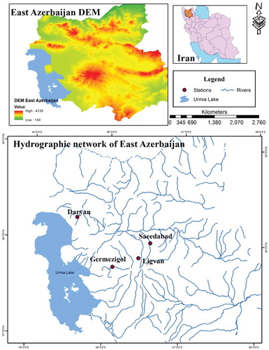
Figure 2. The average annual values of monthly streamflow of all stations.
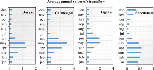
Table 1. Spatial characteristics of stations.
Statistical characteristics of monthly streamflow time series of the case study stations in both calibration and validation stages are shown in Table . The statistical characteristics consist of mean, standard deviation, skewness and kurtosis coefficients, and the lag-one autocorrelation coefficient. The highest amount for correlation is stated in Saeedabad station (0.773 and 0.699) in calibration and validation stages, respectively.
Table 2. Statistical characteristics of studied stations in both calibration and validation stages.
2.2. GEP model
As stated above, GEP, first announced by (Ferreira, Citation2001), is one of the popular DDMs that are in the group of artificial intelligence models based on theories in Darwinian evolution algorithms that they deal with neurons of the human brain. These algorithms tried to search for the best solution, which has the best fit among the other solutions. Each solution is stated as an individual. Weak quality solutions are eliminated by using fitness functions (Ashrafian et al., Citation2020). In the GEP model, chromosomes are performed as an expression tree, and they can be coded by linking functions. The results of the GEP model could be reported by mathematical equations and decision tree structures, while they are a correlation of the input variables of the user. GEP is an application that directly represents genes. GEP selected each gene’s terminals in random behavior. These terminals are extracted from the head and tail of each gene. Terminals are essential because they help the model modification for developing next-generation and evolution process. GEP establishes an original problem set with the first individual names ‘parent node’ this individual multiply to ‘offspring node’ with new top-performance operators. The genetic information of each parent transfers to a new generation with new modified environmental adaption, and it resulted in better fitness. GEP tries to find the best offspring node with a low error. In this way, the evolutionary process grows in a better way.
The main advantages of the GEP model can be discussed as follows (a) chromosomes are small, easy to recombine, mutate, duplicate; (b) The generated decision trees are units of their chromosomes and based on fitness, they selected to reproduce modified chromosomes (Conditioning et al., Citation2019). The main steps in modeling by GEP are summarized in six steps. (1) selecting the fitness function like RMSE, (2) selecting input variables in order to engender chromosomes, (3) choosing operators, (4) scheming the design of chromosomes, (5) choosing the linking functions, and in the last step, (6) choosing the genetic operators (Rahmani-rezaeieh et al., Citation2019). More information can be found in (Ferreira, Citation2001).
2.3. ARCH model
Streamflow time series is defined as the volume of water, which varies in time, which is volatile and has fluctuations in time. Modeling streamflow time series has the principal purpose that we can have insights on data and can forecast or predict that variable. Meanwhile, modeling, the main focus is on the average of used data. However, for modeling hydrological data, significantly streamflow variance of data should be considered. So models that can use the variances of data become highlighter than the others. ARCH was first introduced by (Engle, Citation1982). ARCH model is one of the abovementioned models that deal with a variance of data. This model can consider the parsimonious effects of observed data and provides a framework that is considered nonlinear volatility in data (Hamilton, Citation1994). Equations (1) and (2) illustrate the ARCH model (Bollerslev et al., Citation1994).
(1)
(1)
(2)
(2) Where
is conditional variance,
is a discrete-time stochastic process, and
are the ARCH model’s parameters, q is the model’s order, and zt is the regular and standard series.
2.4. SETAR model
TAR models are dealt with nonlinear systems in a discrete time scale, also considers anomalies’, fluctuations, and seasonality of proposed data. This method was first developed by (Tong, Citation1983a). This model is also called the regime-switching model, which has a value of the threshold for switching between the upper regime and the lower regime of streamflow. These models have Kth parts of AR (p) models in which each part is different from the other parts, and p shows the order of AR models. TAR models can be depicting by TAR (k, p). The whole modeling process is consisting of four main steps; (a) model developing, (b) statical identification, (c) parameters estimation (d) predicting (Pan et al., Citation2017).
SETAR is a nonlinear time series in the family of TAR models (Tong, Citation2015). These models are supposed to use in modeling and forecasting streamflow because of their nonlinearity characteristics. SETAR models have some advantages which make them popular such as considering time irreversibility, jump and chaos phenomena, the harmonic bias in data. Therefore, SETAR models are an excellent tool for modeling a parsimonious non-linear time series (Gonzalo & Wolf, Citation2005). This model also can have two or more regimes depending on the levels of lagged variables in its structure. Using SETAR models by considering two high and low regimes was defined by (Tong, Citation1983b). In the current study, the SETAR model was used in predicting monthly streamflow, divided streamflow time series data into sub-regimes (two regimes). This method is another way of developing nonlinear dynamical methods (Tongal, Citation2013). Streamflow time series data set with (Q1 … ,Qn), in which n is the number of time series, considering two regime SETAR model can be defined by Equations (3) and (4) as follows:
(3)
(3)
(4)
(4) Where
are the coefficients of the AR model, p1 and p2 are the orders of AR models for lower and upper regimes in a two-regime SETAR model, d is a lag or delay time,
is the residual value at time t.
If the threshold variable is chosen as the lagged value of , then it can be written as SETAR (d,p1,p2, … ,pj). The threshold values can be selected from (−∞, ∞) and the threshold (r) and the delay (d) parameters are an experimental procedure that they can be used to select the most proper model for a time series by minimizing the AIC (Tongal & Berndtsson, Citation2017). Based on Tongal (Tongal, Citation2013), because of simplicity, efficiency, and lower computational process, the two regime SETAR were selected in this study.
2.5. Development and integration procedure of models
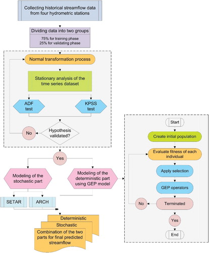
In general, pre-processing is a fundamental step in analyzing historical time series data in various phases, such as designing, application, and methodologies of new models. Data pre-processing techniques could be divided into five groups, including stationary tests, independence tests, normality tests, periodic estimation, consistency, and homogeneity tests. More information about these tests was discussed in (hydrology & 1993, Citationn.d.). Figure demonstrates the whole study steps flowchart. In order to start modeling, the very first step is to collecting streamflow data from hydrometric stations. The next step, splitting the historical data into two segments of calibration and validation phases, is another critical step in every modeling. To reach the best relationship between input and output data, the calibration step is one of the essential parts in modeling (Tongal, Citation2013). As mentioned before, in this study, the streamflow data for each station were split into 75% calibration and 25% validation. The next step is the data-normalization step in which Delleur and Karamouz equations were used for the normalization step in this study. More information can be found (Attar et al., Citation2020). The next step is checking if the data have any trend or seasonality effects or not. When the statistical characteristics (mean, variance, autocorrelation) of historical time series data are all constant over some time, and there is no trend in data series, data series are called stationary. In the current study, the stationary of data was evaluated by two critical tests, including unit-root test augmented dickey-fuller (ADF) and Kwiatkowski–Phillips–Schmidt–Shin (KPSS) test. A unit root test of data series was done by ADF null hypothesis that shows the process has a unit root, and the alternative hypothesis has no unit root, and that means the data series are stationary, and the result of the test is always a negative number. The degree of negativity of this number shows the degree of stationary data. A stationary around means that is tested by the KPSS model, and in contrast with the ADF test, the null hypothesis in KPSS is that the data is stationary, and the alternative hypothesis is that the data is not stationary and the process has a unit root.
Figure 3. The proposed Flow chart in this study.
Moreover, in order to start modeling with nonlinear methods, the LR was used in this study. LR test can discover nonlinearity by using AR(p) and TAR(P) model. The model with AR(p) is the null hypothesis of the LR model, and the alternative hypothesis is modeling with TAR(p).
A vigorous model was achieved when the optimum lags were considered in each modeling scenario. The proper number of lags for each scenario is entirely dependent on input streamflow data. It can be defined based on autocorrelation analysis (partial autocorrelation) methods. There are some steps to defining the optimal number of lags (a) normalization of data, (b) data stationaries, (c) autocorrelation analysis (which lags can be defined based on pacf diagrams in the confidence level of 95%).
In the present study, in order to develop GEP models, each model needs a series of sorted and complete data with defined lags as input data. The input data were considered with five lags (months) for modeling standalone GEP as follows:
The foremost motive for choosing the GEP model is because to create a deterministic equation with different input values while utilizing user-defined linking functions.
As stated before, the procedure of modeling streamflow data with the GEP model considers the mathematical equation of model based on historical time-series data through defined lags by a user. Thus, the main focus on streamflow as a stochastic random phenomenon is hidden while using a standalone GEP model. For this reason, in this study, two models were introduced for modeling random parts of the equation, namely ARCH and SETAR models. In this direction, ARCH and SETAR models consider the variance of the observed data besides considering the statistical mean of streamflow data. Herein, after defining both the deterministic and random parts of the streamflow data using GEP, ARCH, and SETAR models, new series were generated by combining these parts. The combined GEP-ARCH hybrid based model can be defined as:
(5)
(5) Where,
is the modeled deterministic part of the streamflow time-series by GEP and
is the modeled random part of the streamflow series by ARCH. As shown in Equation (5), the equation obtained from GEP models and the results of ARCH modeling is considered as
and
respectively. The combined GEP-SETAR hybrid based model can be defined as:
(6)
(6)
Where, is the modeled deterministic part of the streamflow time-series by GEP and
is the modeled random part of the streamflow series by SETAR. As shown in Equation (6), the equation obtained from GEP models and the results of SETAR modeling is considered as
and
respectively.
3. Assessment of models
In practice, for rigorous accuracy, selecting the most effective and reliable model is an essential task. The accuracy of models can be examined by evaluation criteria. To find the best model, it is necessary to examine these criteria. The evaluation criteria used in this study were the coefficient of determination (R2), root mean square error (RMSE), and mean absolute error (MAE), which can be formulated as follows:
(7)
(7)
(8)
(8)
(9)
(9) Where N is the number of observations,
are the actual observations of streamflow,
is the mean of the observed data, and Pi is the estimated value of streamflow.
4. Results and discussions
In the present study, the benchmark and proposed prediction hybrid models were established using two novel variance-based stochastic nonlinear methods, namely ARCH and SETAR combining with selected best fitted standalone GEP model for four selected hydrometric stations in the Urmia Lake basin. This result part is divided into subsections, including the results of pre-modeling tests, assessment of standalone SETAR models, the results of combined GEP-ARCH and GEP-SETAR models, and in last, the conclusion and future works were recommended.
4.1. Pre-modeling tests
In order to test if the data are stationary and have the potential to nonlinearity modeling, three tests, including ADF, KPSS, and LR tests, examined with a specific hypothesis for each test.
The results of these tests, demonstrated in Table , were showed that by examining their p-value amounts, all data are stationary, and the series has a nonlinearity indefinite significance level. For instance, in Daryan station, the alternative hypothesis is accepted under a 95% confidence level, which means that the series is stationary. The KPSS test is on the other side of the ADF test, which means that based on Table , the null hypothesis is accepted, which means that the data series is stationary under a 95% confidence level. In the case of the likelihood ratio (LR) test, the alternative hypothesis is accepted, which means that the streamflow data series is nonlinear, and SETAR models can fit them.
Table 3. Stationarity (ADF and KPSS) and threshold nonlinearity tests (LR) for proposed stations.
4.2. Assessment of applied standalone nonlinear SETAR models
Before starting SETAR modeling, the threshold and delay parameters with the orders of AR models should be firstly estimated. In order to test data independence and orders, ACF and PACF figs were calculated. The degree of SETAR models was estimated by PACF. Also, the satisfactoriness of SETAR models is established when all the ACF coefficients were located between confidence intervals.
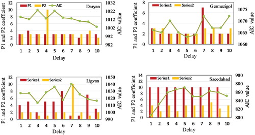
As shown in Figure , the orders for monthly streamflow for all the stations can be defined (four lags for Daryan, Germezigol, Ligvan stations, and two lags for Saeedabad station). They directed that the SETAR models are useful for monthly streamflow modeling. Next, delay (d), order values (P1, P2), and the threshold value (regime-switching threshold value) was estimated based on the minimum AIC criterion. These values for each station are shown in Figure . For instance, in Daryan station the SETAR model values (d = 10, P1 = 3, P2 = 2), for Germezigol station (d = 5, P1 = 2, P2 = 2), for Ligvan stations (d = 3, P1 = 2, P2 = 1) and for Saeedabad station (d = 1, P1 = 10, P2 = 4) were calculated.
Figure 4. Autocorrelation and partial autocorrelation of standardized monthly streamflow time series for Daryan, Germezigol, Ligvan, Saeedabad stations, respectively.
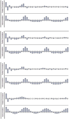
Figure 5. Delay (d) (y-axis), order (P1, P2), AIC values for Daryan, Germezigol, Ligvan, and Saeedabad stations.
Based on the obtained delay parameters and order values from Figure , the threshold value for SETAR models based on Equations (5) and (6) are calculated for each station. Equations (10–13) illustrate the results of two regime SETAR models for all stations including Daryan, Germezigol, Ligvan, Saeedabad with SETAR (2,3,2), SETAR (2,1,2), SETAR (2,2,1) and SETAR (2,2,2) respectively. The complementary information like the order, the delay parameter, and threshold values for each station can be obtained from these equations. In the equation number 10, the equation (-0.2374
+0.206
) with the threshold of
shows the lower regime of the SETAR model. While the
with the threshold of
shows the upper regime. The behavior of the basin can be determined based on these threshold values of streamflow data. As if, streamflow water level surpassed the threshold value, it increases the runoff probability in the basin. In opposite, if the stream flow water level is below (when there is little precipitation) the threshold value, then drought would happen.
(10)
(10) Results of fitted SETAR two-regime models to the monthly streamflow Datasets of Germezigol station with SETAR (2,1,2)
(11)
(11) Results of fitted SETAR two-regime models to the monthly streamflow Datasets of Ligvan station with SETAR (2,2,1)
(12)
(12) Results of fitted SETAR two-regime models to the monthly streamflow Datasets of Saeedabad station with SETAR (2,2,2)
(13)
(13)
Where and
are the streamflow with the lags of 1 and two months, respectively.
4.3. Assessment of applied combined models
The following values were considered in this study for the input variables of the GEP model. Number of Genes = 3, number of chromosomes = 30, head size = 8, mutation rate = 0.04, inversion rate = 0.1, gene recombination rate = 0.1, one-point recombination rate = 0.3, two-point recombination rate = 0.3, Gene transposition rate = 0.1, insertion sequence transposition rate = 0.1, root insertion sequence transposition rate = 0.1. Then, as formerly explained, in this study GEP model, combined by nonlinear time series models, including SETAR and ARCH models. In this part, the results of the study were divided into two sections, namely GEP-ARCH and GEP-SETAR combinations.
4.3.1. GEP-ARCH combination
Figures – demonstrate the time series plots for each station in a combination of GEP lags with ARCH models. As shown in Figure , the observed streamflow (black lined) were compared with all models; it could be concluded that GEP5-ARCH is closer to observed values.
Figure 6. Time series for Daryan station.
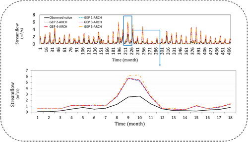
Figure 7. Time series for Germezigol station.
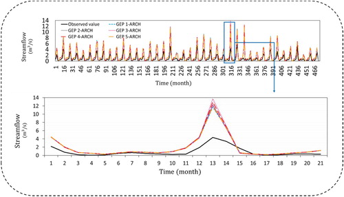
Figure 8. Time series for Ligvan station.
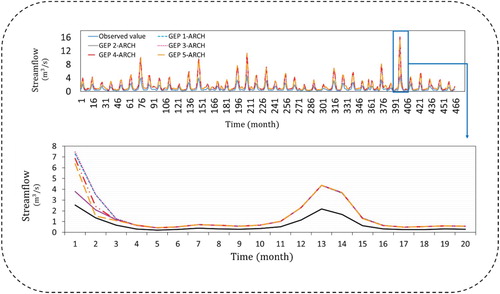
Figure 9. Time series for Saeedabad station.
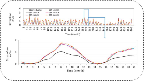
Tables – represent the obtained performance criteria of each combination of different lags of the GEP model with nonlinear ARCH models. As shown in the following tables, evaluation indices have convincing results for each combination in both calibration and validation stages. In Daryan hydrometric station, in the calibration stage GEP5-ARCH model with the correlation coefficient values of (R2 = 0.737) error values of (RMSE = 0.042 m3/s and MAE = 0.475 m3/s) have selected as the top model. Same GEP5-ARCH model in validation stage (R2 = 0.477, RMSE = 0.079 m3/s and MAE = 0.464 m3/s) were selected. In Germezigol station GEP3-ARCH model is selected as the best model in both calibration and validation stages with the values of R2 = 0.804, RMSE = 0.083 m3/s, MAE = 0.945 m3/s for calibration and R2 = 0.845, RMSE = 0.109 m3/s, MAE = 0.778 m3/s for testing phases. In Ligvan station, GEP model with one lag (GEP1) was combined with ARCH model resulted R2 = 0.977, RMSE = 0.068 m3/s, MAE = 0.881 m3/s in calibration stage and R2 = 0.929, RMSE = 0.147 m3/s, MAE = 0.925 m3/s in validation stage. In Saeedabad station, the values of R2 = 0.907, RMSE = 0.018 m3/s, MAE = 0.267 m3/s in calibration stage and R2 = 897, RMSE = 0.022 m3/s, MAE = 0.170 m3/s made GEP2-ARCH model the most fitted model with observed monthly streamflow values.
Table 4. The results of hybrid models in Daryan station.
Table 5. The results of hybrid models in Germezigol station.
Table 6. The results of hybrid models in Ligvan station.
Table 7. The results of hybrid models in Saeedabad station.
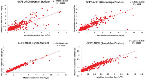
In this section, the observed and modeled data of each GEP-ARCH combination based on their coefficient of efficiency values were shown by Figure . Scatter plots of the observed monthly streamflow values against estimated with hybrid GEP-ARCH models resulted in satisfactory and acceptable values for each station.
Figure 10. Combined best performed GEP-ARCH model for all Stations.
4.3.2. GEP-SETAR combination
Figures – show the time series plots for each station of Daryan, Germezigol, Ligvan, and Saeedabad.
Figure 11. Time series for GEP-SETAR for Daryan station.
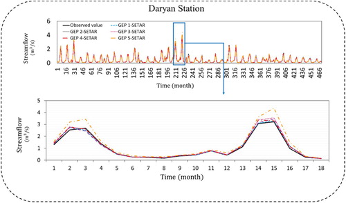
Figure 12. Time series for GEP-SETAR for Germezigol station.

Figure 13. Time series for GEP-SETAR for Ligvan station.
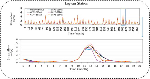
Figure 14. Time series for GEP-SETAR for Saeedabad station.
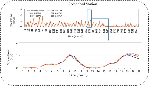
Tables – represent the obtained performance criteria of each combination of different lags of the GEP model with nonlinear two regime SETAR models. As shown in these tables, evaluation indices have convincing results for each combination in both calibration and validation stages.
Table 8. The results of hybrid models in Daryan station.
Table 9. The results of hybrid models in Germezigol station.
Table 10. The results of hybrid models in Ligvan station.
Table 11. The results of hybrid models in Saeedabad station.
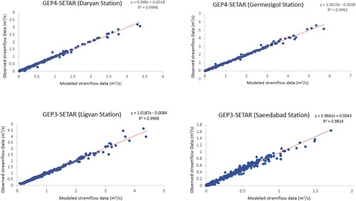
In Daryan station, GEP4-SETAR model was selected as best performed model among others because of evaluation indices, R2 = 0.995, RMSE = 0.002 m3/s, MAE = 0.017 m3/s for calibration station and R2 = 991, RMSE = 0.003 m3/s, MAE = 0.025 m3/s for validation stages. In Table , GEP4-SETAR model was selected as the top model with the values of R2 = 0.997, RMSE = 0.003 m3/s, MAE = 0.026 m3/s for calibration stages and R2 = 0.993, RMSE = 0.007 m3/s, MAE =0.033 m3/s in testing stages. Based on values of R2 =0.996, RMSE = 0.002 m3/s, MAE = 0.021 m3/s for calibration stages in Ligvan station the GEP2-SETAR model were selected while GEP3-SETAR model in validation stage was selected based on values of R2 = 0.979, RMSE = 0.009 m3/s, MAE = 0.040 m3/s. GEP3-SETAR model was selected for Saeedabad station with these values of R2 = 0.979, RMSE = 0.002 m3/s, MAE =0.027 m3/s for calibration and R2 = 0.981, RMSE =0.002 m3/s, MAE = 0.014 m3/s for validation stages.
In this section, the observed and modeled data of each GEP-SETAR combination based on their coefficient of efficiency values were shown in Figure . The results showed satisfactory and acceptable values for each station by considering the calibration and validation stages. In comparison to GEP-ARCH type hybrid models, these combined GEP-SETAR models have very high values of correlation between observed and estimated values. Therefore, SETAR type models perform better than hybrid ARCH methods.
Figure 15. Combined best performed GEP-SETAR model for all Stations.
4.4. Comparison between selected ARCH-type and SETAR type models
As shown in previous sections, two deterministic and stochastic parts of both GEP and time-series models combined by Equations (5) and (6). As an example of Daryan station, the results of combined GEP-ARCH models in both calibration and validation stages show (R2 = 0.737, RMSE = 0.042 m3/s, and MAE = 0.475 m3/s) and (R2 = 0.477, RMSE =0.079 m3/s, and MAE = 0.464 m3/s) respectively. While the results of combined GEP-SETAR models in both calibration and validation stages in Table shows (R2 = 0.995, RMSE = 0.002 m3/s, and MAE =0.017 m3/s) and (R2 = 0.991, RMSE = 0.003 m3/s and MAE = 0.011 m3/s) respectively.
5. Discussion
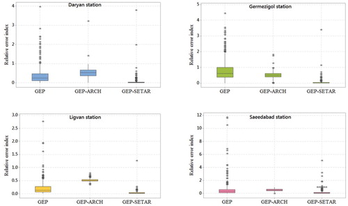
In this study, the concept of nonlinearity, parsimonious, and complexity of monthly streamflow data was considered for defining the superior model. At the first step, 40 years of streamflow data with the 30 days (monthly) scale were selected from four rivers located in ULB. Streamflow data were modeled with GEP methods (including five different scenarios and inputs), and the equations and the estimated data were defined, and they compared with the historical data in two calibration and validation stages. It is clear that the GEP model has the capacity to model the linear and nonlinear relations between the input variables. Also, the GEP only exported the deterministic components of the streamflow equations. Considering both deterministic and stochastic concepts of every hydrological model. Here, in this study, ARCH models were combined with the best performed GEP model, and the results were reported. In the next step, in order to find the mean behavior of streamflow data and the changes between upper and lower regime types (switching regimes) and considering the threshold between them, SETAR models were utilized. Finally, the results of SETAR models were combined with superior GEP models, and the results showed a satisfying and acceptable increase in the models’ performances in comparison to hybrid GEP-ARCH models based on evaluation criteria. In other words, to address these findings, the relative error index was calculated and depicted in Figure for all the proposed stations. For Daryan station, as it shown in blue box plots, the error plots were demonstrated that the GEP-SETAR has the lowest value following the standalone GEP and the hybrid GEP-ARCH models. In Germezigol station (green error box plots), it can be seen that both hybrid models, including ARCH type and SETAR type models, performed better than the sole GEP model. Yellow color error box plots reveal the relative error-index between 0 and 3, and the GEP-SETAR model draws heavily in comparison to the two other models. Finally, the same results can be seen at the pink color error box plot for Saeedabad station, which presented the lowest error model.
Figure 16. Relative error-index values for Daryan station (blue), Germezigol (green), Ligvan station (yellow) and Saeedabad station (pink).
The overall performance comparison of two regime SETAR models along with ARCH type models for two primary calibration and validation stages were demonstrated in Table . Utilizing the error type (RMSE, MAE) and accuracy type (R2) evaluation metrics, Table demonstrates the ratio of SETAR-type models to ARCH-type models’ performance in percent. Overall, as a significant result, all SETAR-type hybrid models in this study have better performance than ARCH-type models.
Table 12. The preference of hybrid GEP-SETAR models to hybrid GEP-ARCH models.
6. Conclusion and future works
Nowadays, providing a method for enhancing hydrological forecasting accuracy is a challenging issue for engineers and scholars in water resources planning and management. Relatively, with the literature review, there is little attention in utilizing both deterministic DDMs and stochastic time series for forecasting hydrological parameters, especially streamflow. In this study, the predictability of newly hybrid applied DDMs from monthly streamflow of four stations, Daryan, Germezigol, Ligvan, and Saeedabad, at Urmia basin was assessed using performance metrics called R2, RMSE, and MAE and visual plots. One commonly used DDM called GEP was used in this study as a primary deterministic model, while two-time series models called ARCH and SETAR models as nonlinear models as a stochastic determination parts were used. By comparing the latest results of best performed GEP and ARCH and SETAR models, it is found out that in all calibration and validation stages within all stations, SETAR models have the best performance, comparing to ARCH models. In terms of accuracy, prediction results for Daryan, Germezigol, Ligvan, and Saeedabad, respectively, improved by about 51%, 15%, 1%, and 2% when the GEP model integrated with SETAR compared to ARCH. In addition, the RMSE value for the ratio of the SETAR-type models to ARCH-type models decreased to 45% (Daryan), 74 (Germezigol), 88% (Ligvan), and 16% (Saeedabad) at the validation stage. Overall, it can be stated that hybrid GEP-SETAR models are demonstrated improving classical models, and they can be used for analyzing, modeling, and predicting stream flows for future water management.
For future studies, it can be useful to consider other statistics like mean and kurtosis using new methods such as SETARMA, BL, BL-ARCH, or other autoregressive conditional heteroscedasticity models such as GARCH, partial autoregressive conditional heteroscedasticity (PARCH), Non-linear GARCH. In contrast, this study applied the variance statistics of observed streamflow data. Another suggestion is for data decomposition as nonlinearity, non-stationary, complexity, and random distribution can be seen on hydrological processes (i.e. streamflow, rainfall, water stage, groundwater, etc.). To overcome those difficulties, several data pre-processing tools such as complete ensemble empirical mode decomposition (CEEMD), improved CEEMD, and variational mode decomposition (VMD), can be addressed.
Acknowledgements
We acknowledge the ‘Open Access Funding by the Publication Fund of the TU Dresden’.
Disclosure statement
No potential conflict of interest was reported by the author(s).
Additional information
Funding
References
- Abdollahi, S., Raeisi, J., Khalilianpour, M., Ahmadi, F., & Kisi, O. (2017). Daily mean streamflow prediction in perennial and non-perennial rivers using four data driven techniques. Water Resources Management, 31, 4855–4874. https://doi.org/10.1007/s11269-017-1782-7
- Abdulelah Al-Sudani, Z., Salih, S. Q., Sharafati, A., & Yaseen, Z. M. (2019). Development of multivariate adaptive regression spline integrated with differential evolution model for streamflow simulation. Journal of Hydrology, 573, 1–12. https://doi.org/10.1016/j.jhydrol.2019.03.004
- Ahani, H., & Kherad, M. (2013). Non-parametric trend analysis of the aridity index for three large arid and semi-arid basins in Iran. 553–564. https://doi.org/10.1007/s00704-012-0747-2
- Ahani, A., Shourian, M., & Rahimi Rad, P. (2018). Performance assessment of the linear, nonlinear and nonparametric data driven models in river flow forecasting. Water Resources Management, 32(2), 383–399. https://doi.org/10.1007/s11269-017-1792-5
- Ashrafian, A., Gandomi, A. H., Rezaie-Balf, M., & Emadi, M. (2020). An evolutionary approach to formulate the compressive strength of roller compacted concrete pavement. Measurement: Journal of the International Measurement Confederation, 152, 107309. https://doi.org/10.1016/j.measurement.2019.107309
- Attar, N. F., Pham, Q. B., Nowbandegani, S. F., Rezaie-Balf, M., Fai, C. M., Ahmed, A. N., Pipelzadeh, S., Dung T. D., Nhi P. T. T., Khoi D. N., & El-Shafie, A. (2020). Enhancing the prediction accuracy of data-driven models for monthly streamflow in Urmia Lake basin based upon the autoregressive conditionally heteroskedastic time-series model. Applied Sciences, 10(2), 571. https://doi.org/10.3390/app10020571
- Banihabib, M. E., Bandari, R., & Peralta, R. C. (2019). Auto-regressive neural-network models for long lead-time forecasting of daily flow. Water Resources Management, 33(1), 159–172. https://doi.org/10.1007/s11269-018-2094-2
- Bollerslev, T., Engle, R. F., & Nelson, D. B. (1994). Handbook of econometrics. Handbook of Econometrics, 4, 2959–3038. https://doi.org/10.1016/S1573-4412(05)80018-2
- Chang, T., Talei, A., Chua, L., & Alaghmand, S. (2019). The impact of training data sequence on the performance of neuro-fuzzy rainfall-runoff models with online learning. Water, 11(1), 52. https://doi.org/10.3390/w11010052
- Chen, C.-S., Liu, C.-H., and Su, H.-C. (2008). A nonlinear time series analysis using two-stage genetic algorithms for streamflow forecasting.
- Conditioning, O., Using, F., Mapping, P., Sahin, E. K., Colkesen, I., Rahmati, O., … Daneshi, A. (2019). Groundwater potential mapping at Kurdistan region of Iran using analytic hierarchy process and GIS. Journal of Hydrology, 31(June), 1–21. https://doi.org/10.1007/s12517-014-1668-4
- Das, B. S., Devi, K., & Khatua, K. K. (2019). Prediction of discharge in converging and diverging compound channel by gene expression programming. ISH Journal of Hydraulic Engineering. https://doi.org/10.1080/09715010.2018.1558116
- Diop, L., Bodian, A., Djaman, K., Yaseen, Z. M., Deo, R. C., El-shafie, A., & Brown, L. C. (2018). The influence of climatic inputs on stream-flow pattern forecasting: Case study of upper senegal river. Environmental Earth Sciences, 77(5). https://doi.org/10.1007/s12665-018-7376-8
- Engle, R. F. (1982). Autoregressive conditional heteroscedasticity with estimates of the variance of United Kingdom Inflation. Econometrica, 50(4), 987. https://doi.org/10.2307/1912773
- Fathian, F., Fakheri Fard, A., Ouarda, T. B. M. J., Dinpashoh, Y., & Mousavi Nadoushani, S. S. (2019, October). Modeling streamflow time series using nonlinear SETAR-GARCH models. Journal of Hydrology, 573, 82–97. https://doi.org/10.1016/j.jhydrol.2019.03.072
- Ferreira, C. (2001). Gene expression programming in problem solving. Soft Computing in Industry – Recent Applications, (1996), 641–660. https://doi.org/10.1007/978-1-4471-0123-9_54
- Freire, P. K. d. M. M., Santos, C. A. G., & Silva, G. B. L. d. (2019). Analysis of the use of discrete wavelet transforms coupled with ANN for short-term streamflow forecasting. Applied Soft Computing Journal, 80, 494–505. https://doi.org/10.1016/j.asoc.2019.04.024
- Ghorbani, M. A., Khatibi, R., Karimi, V., Yaseen, Z. M., & Zounemat-Kermani, M. (2018). Learning from multiple models using artificial intelligence to improve model prediction accuracies: Application to river flows. Water Resources Management, 32(13), 4201–4215. https://doi.org/10.1007/s11269-018-2038-x
- Ghose, D. K., & Samantaray, S. (2019). Estimating runoff using feed-forward neural networks in scarce rainfall region. https://doi.org/10.1007/978-981-13-1921-1_6
- Gonzalo, J., & Wolf, M. (2005). Subsampling inference in threshold autoregressive models. Journal of Econometrics, 127(2), 201–224. https://doi.org/10.1016/j.jeconom.2004.08.004
- Hamilton, D. (1994). Autoregressive conditional heteroskedasticity and changes in regime. Journal of Econometrics, 64(1–2), 307–333. https://doi.org/10.1016/0304-4076(94)90067-1
- Honorato, A. G. d. S. M., Silva, G. B. L. d., & Guimarães Santos, C. A. (2019). Monthly streamflow forecasting using neuro-wavelet techniques and input analysis. Hydrological Sciences Journal, 63(15–16), 2060–2075. https://doi.org/10.1080/02626667.2018.1552788
- hydrology, J. S.-H. of, & 1993, undefined. (n.d). Analysis and modelling of hydrological time series. Ci.Nii.Ac.Jp. http://ci.nii.ac.jp/naid/10013176141/
- Kiafar, H., Babazadeh, H., Marti, P., Kisi, O., Landeras, G., Karimi, S., & Shiri, J. (2017). Evaluating the generalizability of GEP models for estimating reference evapotranspiration in distant humid and arid locations. Theoretical and Applied Climatology, 130, 377–389. https://doi.org/10.1007/s00704-016-1888-5
- Kisi, O., Choubin, B., Deo, R. C., & Yaseen, Z. M. (2019). Incorporating synoptic-scale climate signals for streamflow modelling over the Mediterranean region using machine learning models. Hydrological Sciences Journal, 64(10), 1240–1252. https://doi.org/10.1080/02626667.2019.1632460
- Kisi, O., Karimi, S., Shiri, J., Makarynskyy, O., & Yoon, H. (2014). Forecasting sea water levels at Mukho station, South Korea using soft computing techniques. The International Journal of Ocean and Climate Systems, 5(4), 175–188. https://doi.org/10.1260/1759-3131.5.4.175
- Komorník, J., Komorníková, M., Mesiar, R., Szökeová, D., & Szolgay, J. (2006). Comparison of forecasting performance of nonlinear models of hydrological time series. Physics and Chemistry of the Earth, 31(18), 1127–1145. https://doi.org/10.1016/j.pce.2006.05.006
- Li, X., Sha, J., Li, Y. M., & Wang, Z. L. (2018). Comparison of hybrid models for daily streamflow prediction in a forested basin. Journal of Hydroinformatics, 20(1), 206–220. https://doi.org/10.2166/hydro.2017.010 doi: 10.2166/hydro.2017.189
- Liang, Z., Tang, T., Li, B., Liu, T., Wang, J., & Hu, Y. (2018). Long-term streamflow forecasting using SWAT through the integration of the random forests precipitation generator: Case study of Danjiangkou reservoir. Hydrology Research, 49(5), 1513–1527. https://doi.org/10.2166/nh.2017.085
- Mahmood Al-Juboori, A., & Guven, A. (2016). A stepwise model to predict monthly streamflow. Journal of Hydrology, 543, 283–292. https://doi.org/10.1016/j.jhydrol.2016.10.006
- Pan, J., Xia, Q., & Liu, J. (2017). Bayesian analysis of multiple thresholds autoregressive model. Computational Statistics, 32(1), 219–237. https://doi.org/10.1007/s00180-016-0673-3
- Prasad, R., Deo, R. C., Li, Y., & Maraseni, T. (2017). Input selection and performance optimization of ANN-based streamflow forecasts in the drought-prone Murray Darling basin region using IIS and MODWT algorithm. Atmospheric Research, 197, 42–63. https://doi.org/10.1016/j.atmosres.2017.06.014
- Rahmani-rezaeieh, A., Mohammadi, M., & Mehr, A. D. (2019). Ensemble gene expression programming: A new approach for evolution of parsimonious streamflow forecasting model (2002).
- Ravansalar, M., Rajaee, T., & Kisi, O. (2017). Wavelet-linear genetic programming: A new approach for modeling monthly streamflow. Journal of Hydrology, 549, 461–475. https://doi.org/10.1016/j.jhydrol.2017.04.018
- Ren, W. W., Yang, T., Huang, C. S., Xu, C. Y., & Shao, Q. X. (2018). Improving monthly streamflow prediction in alpine regions: Integrating HBV model with Bayesian neural network. Stochastic Environmental Research and Risk Assessment, 32(12), 3381–3396. https://doi.org/10.1007/s00477-018-1553-x
- Shiri, J., Kişi, Ö, Makarynskyy, O., Shiri, A. A., & Nikoofar, B. (2012). Forecasting daily stream flows using artificial intelligence approaches. ISH Journal of Hydraulic Engineering, 18(3), 204–214. https://doi.org/10.1080/09715010.2012.721189
- Szolgayová, E. P., Danačová, M., Komorniková, M., & Szolgay, J. (2017). Hybrid forecasting of daily river discharges considering autoregressive heteroscedasticity. Slovak Journal of Civil Engineering, 25(2), 39–48. https://doi.org/10.1515/sjce-2017-0011
- Tian, Y., Xu, Y. P., Yang, Z., Wang, G., & Zhu, Q. (2018). Integration of a parsimonious hydrological model with recurrent neural networks for improved streamflow forecasting. Water (Switzerland), 10(11). https://doi.org/10.3390/w10111655
- Tikhamarine, Y., Souag-gamane, D., Ahmed, A. N., Kisi, O., & El-shafie, A. (2019). Improving artificial intelligence models accuracy for monthly streamflow forecasting using Grey Wolf Optimization (GWO) algorithm. Journal of Hydrology, 124435. https://doi.org/10.1016/j.jhydrol.2019.124435
- Tikhamarine, Y., Souag-Gamane, D., & Kisi, O. (2019). A new intelligent method for monthly streamflow prediction: Hybrid wavelet support vector regression based on grey wolf optimizer (WSVR–GWO). Arabian Journal of Geosciences, 12(17). https://doi.org/10.1007/s12517-019-4697-1
- Tong, H. (1983a). Threshold models in non-linear time series analysis. Springer.
- Tong, H. (1983b). Threshold models in non-linear time series analysis. https://doi.org/10.1007/978-1-4684-7888-4
- Tong, H. (2015). Nonlinear time series analysis (pp. 1–7).
- Tongal, H. (2013). Nonlinear dynamical approach and self-exciting threshold model in forecasting daily stream-flow. Fresenius Environmental Bulletin, 22(10), 2836–2847.
- Tongal, H., & Berndtsson, R. (2014). Phase-space reconstruction and self-exciting threshold modeling approach to forecast lake water levels. Stochastic Environmental Research and Risk Assessment, 28(4), 955–971. https://doi.org/10.1007/s00477-013-0795-x
- Tongal, H., & Berndtsson, R. (2017). Impact of complexity on daily and multi-step forecasting of streamflow with chaotic, stochastic, and black-box models. Stochastic Environmental Research and Risk Assessment, 31(3), 661–682. https://doi.org/10.1007/s00477-016-1236-4
- Xu, J., Zhang, W., & Zhao, J. (2009, June 12–16). Stream flow forecasting by artificial neural network and TOPMODEL in Baohe River basin. 3rd International Symposium on Intelligent Information Technology Application Workshops, IITAW 2009 (pp. 186–189). https://doi.org/10.1109/IITAW.2009.27
- Yaghoubi, B., Hosseini, S. A., & Nazif, S. (2019). Monthly prediction of streamflow using data-driven models. Journal of Earth System Science, 128(6). https://doi.org/10.1007/s12040-019-1170-1
- Yaseen, Z. M., Allawi, M. F., Yousif, A. A., Jaafar, O., Hamzah, F. M., & El-Shafie, A. (2018). Non-tuned machine learning approach for hydrological time series forecasting. Neural Computing and Applications, 30(5), 1479–1491. https://doi.org/10.1007/s00521-016-2763-0
- Yaseen, Z. M., Awadh, S. M., Sharafati, A., & Shahid, S. (2018, October). Complementary data-intelligence model for river flow simulation. Journal of Hydrology, 567, 180–190. https://doi.org/10.1016/j.jhydrol.2018.10.020
- Yaseen, Z. M., Ebtehaj, I., Bonakdari, H., Deo, R. C., Danandeh Mehr, A., Mohtar, W. H. M. W., Diop, L., El-shafie, A., & Singh, V. P. (2017). Novel approach for streamflow forecasting using a hybrid ANFIS-FFA model. Journal of Hydrology, 554, 263–276. https://doi.org/10.1016/j.jhydrol.2017.09.007
- Yaseen, Z. M., Sulaiman, S. O., Deo, R. C., & Chau, K. W. (2019). An enhanced extreme learning machine model for river flow forecasting: State-of-the-art, practical applications in water resource engineering area and future research direction. Journal of Hydrology, 569, 387–408. https://doi.org/10.1016/j.jhydrol.2018.11.069
- Yu, X., Wang, Y., Wu, L., Chen, G., Wang, L., & Qin, H. (2020). Comparison of support vector regression and extreme gradient boosting for decomposition-based data-driven 10-day streamflow forecasting. Journal of Hydrology, 582, 124293. https://doi.org/10.1016/j.jhydrol.2019.124293
- Zamani Sabzi, H., King, J. P., & Abudu, S. (2017). Developing an intelligent expert system for streamflow prediction, integrated in a dynamic decision support system for managing multiple reservoirs: A case study. Expert Systems with Applications, 83, 145–163. https://doi.org/10.1016/j.eswa.2017.04.039