Numerical investigation on the crosswind effects on a train running on a bridge

Abstract

With the increase of the running speed of the high-speed train (HST), aerodynamic interference between the HST and surrounding structures becomes more and more important. Traditional wind tunnel experiments using the stationary model can not fully reveal the pulsing behavior of the aerodynamic forces on both the HST and surrounding structures. This paper numerically investigates the aerodynamic characteristics of an HST running on a bridge in cross-wind. The simulation results reveal that when there is no wind barrier, the stationary model case with the yaw angle identical to the moving model case can roughly reproduce the main flow structures around the train. However, once the train runs downstream a wind barrier, the stationary model cannot reveal its aerodynamic characteristics regardless of the yaw angle adopted. The moving model scenario successfully captures the pulsing behavior of the forces on both the train and wind barrier, which is concealed in the cases with a stationary model. The present results indicate that only the moving model method can fully reveal the aerodynamic characteristics and interactions between the train and surrounding structures, especially in evaluating their dynamic response.

KEYWORDS:

• High-speed train
• Bridge
• Wind barrier
• Crosswind
• CFD

1. Introduction

The lateral force on a train is crucial to its stabilization, especially for a high-speed train (HST) running in the strong cross wind. A lot of investigations indicate that strong cross wind may overturn running trains. About 30 wind-induced train accidents were reported in Japan from 1899 to 2006. Particularly, in 1986, a heavy diesel locomotive train was blown off from the Amarube bridge by a strong cross-wind, killing 6 people and wounding 6 others. The investigation on this accident revealed that the interference between the train and bridge must be considered, besides the effects of strong cross wind.

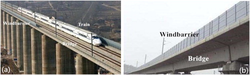
Wind barrier was found to be one of the essential measures to ensure the stability and safety of trains under strong cross-wind. Most of the high-speed railway (HSR) lines that pass through strong windy areas are set additional wind barriers, as shown in Figure 1. Along with the extension of the HSR network, the wind barrier, as a control and protection measure in railway operation, becomes more and more important.

Figure 1. Wind barrier on the bridge: (a) 3D view; (b) side view.

The primary aim of setting up wind barriers is to guarantee the train operation safety. Meanwhile, wind load on the barrier, as well as its wind included vibration, should also be paid adequate attention to. Otherwise, the severe accident may occur because of the damage of wind barriers. For example, part of the wind barrier was blown down to the railway in the Beijing-Shanghai HSR line in 2010, which led to a halt of the whole line. Besides, when a train passes by with a very high speed, the effects of slipstream and shock waves on the wind barrier should also be considered.

In recent years, many researchers did substantive research in the field of the aerodynamic performance of wind barriers, through wind tunnel tests (Guo et al., 2015; He et al., 2014, 2016) and computational fluid dynamic (CFD) simulations (e.g. Catanzaro et al., 2016; He et al., 2018; Krajnović et al., 2012). Guo et al. (2015) investigated the effect on aerodynamic performance for wind barriers with a system of high-speed train and bridge. Effects of height (0, 2.0, 3.5, 5.0 m) and porous ratio (0%, 10%, 30%, 50%) of the barrier were studied systematically. They found that the wind barrier is set at the upstream of the track with a height of 3.5 m and a ventilation rate of 30%, the lateral force and overturning moment coefficients of the vehicle can be efficiently reduced by 71.4% and 78.7%, respectively. Tomasini et al. (2015) studied the combined effects of height and porous ratio of wind barriers on a high-speed train (HST). They found a perforated plate barrier with a height of 3 m and a porous ratio of 33%, and a horizontal band barrier with a height of 4 m and the porous ratio of 50% can both reduce the overturning moment of the train by about 30%. Xiang et al. (2014) studied the wind resistance performance of wind barriers on track sides. Based on large amounts of wind tunnel experiments, covering the height of wind barrier from 1.60 m to 2.90 m and the porous rate from 0 to 40%, they studied the protective effect of wind barrier with data envelopment analysis technique (DEA). A pattern was found, the lift/drag ratio can be increased after a certain high level, the protective effect is strongest when its height is 2.05 m with a porous ratio of 0%. Zhang et al. (2017) tested the aerodynamic force coefficients of a vehicle-bridge system by adjusting different parameters combination, including height (0∼5m) and porous ratio (0∼40%) of barriers. They suggested that the aerodynamic coefficients have no obvious variety regulation on barrier’s heights in their test range, but are closely connected with its porous ratio.

All the investigations mentioned above using stationary train models in their experiments or simulations. Obviously, this configuration does not consider the relative movement and interference between the train and bridge/ground, and it is not appropriate to evaluate the cross-wind stability for an HST. As mentioned previously, the slipstream caused by an HST can result in a severe lateral load on the barrier. Obviously, the test with a stationary model cannot reveal this effect as well. As pointed out by Cooper (1980), the actual effects of wind shear, turbulence, and the influence of the mutual motion between the vehicle model and ground can only be correctly simulated by moving model experiments.

Moving model configuration are widely used in the investigations on the piston effects of a train passing a tunnel. For example, Huang et al. (2010). studied the of train-induced unsteady airflow in a subway tunnel with natural ventilation ducts using CFD. Auvity et al. (2001) focused on the influence of the resulting exit flow created at the tunnel portal on the train through the experiments. Using both field measurement data and CFD results, Xue et al. (2014) analyzed the piston effect and unsteady airflow in a subway station and tunnel caused by a running HST.

With the continuous raising of train speed, slipstream becomes a more and more crucial aerodynamic issue. Recently, four different techniques were used for studying the slipstream, e.g. full-scale field test (2014a, 2014b; Baker, 1991), moving model test (Baker et al., 2001; 2015), wind tunnel test (Bell et al., 2014; Xia et al., 2018) and CFD simulation (Wang et al., 2017; Xia et al., 2016, 2017). The investigations have revealed the connection between the vortex motion and the slipstream in the wake of an HST. However, the lateral load on the wind barrier induced by the slipstream has not been widely studied yet.

Although the full-scale field test is a reliable and feasible method, however, which requires a lot of environmental, safety, and cost concerns. Moving model tests are becoming more acceptable and vogue because it can simulate the real conditions. It needs complex mechanisms and experimental setup to accelerate and decelerate the moving model. Another way to measure and test the slipstream is an experiment in a wind tunnel using the static model, which is the current most widely used because of its simplicity. Nevertheless, the relative motion between vehicle and ground/infrastructure is not considered.

With advances in the technology of the computational hardware and numerical methods (Akbarian et al., 2018; Ghalandari et al., 2019; Mou et al., 2017), CFD becomes applicable in studying the aerodynamic problems of HSTs. Xia et al. (2017) compared the flow structure around an HST for different states of the ground configurations using large eddy simulation (LES). Several other researchers (Hemida et al., 2012; Huang et al., 2014; Muld et al., 2012) had also successfully investigated the slipstream of an HST using CFD. However, few studies concerned about the pressure and lateral load on wind barriers induced by the slipstream when an HST passes by. This problem may become more significant when there is a strong cross-wind because of the combined effect of cross-wind and slipstream.

The aerodynamic force on a running vehicle under cross-wind is usually estimated using wind tunnel tests with stationary models (Premoli et al. 2016). Generally, both the train and infrastructure models are stationary in wind tunnel experiments, which are rotated simultaneously relative to the oncoming wind. That is, both the train and infrastructure have the same yaw angles, which are obviously different from the real case because of the relative motion between them. Moreover, the slipstream caused by train may also influence the aerodynamic forces on the bridge and surrounding structures, e.g. wind/sound barriers. Recently, some moving model tests have been carried out to highlight the unsteady characteristics of the aerodynamic forces caused by a running train under crosswind (Wang et al., 2018; Yao et al., 2020).

In order to further probe into the unsteady aerodynamic forces on a running HST and surrounding wind barrier, the present study investigated these aerodynamic forces for both stationary and moving HST on a bridge. Taking advantages of numerical simulation, cases with different train running conditions and effective yaw angles were compared in detail. Particularly, wind loads on the surrounding barrier were studied in detail for these cases, which reveals the significant unsteady effects caused by the passing HST.

2. Numerical schemes

For the simulation, the air is assumed to be incompressible since the HST speed is under 350 km/h, according to the Ma = V/a = 0.29 < 0.3, where V is the HST speed, and a is the local sound speed, respectively. Navier-Stokes (N-S) equations and mass conservation equations describe the fluid motion: (1) $\begin{array}{rl}& \frac{\mathrm{\partial }\rho }{\mathrm{\partial }\text{t}}+\frac{\mathrm{\partial }(\rho \mathrm{u})}{\mathrm{\partial }\text{x}}+\frac{\mathrm{\partial }(\rho \mathrm{v})}{\mathrm{\partial }\text{y}}+\frac{\mathrm{\partial }(\rho \mathrm{w})}{\mathrm{\partial }\text{z}}=0\end{array}$(1) (2) $\begin{array}{rl}& \frac{\mathrm{\partial }(\rho \mathrm{u})}{\mathrm{\partial }\text{t}}+\frac{\mathrm{\partial }(\rho \mathrm{uu})}{\mathrm{\partial }\text{x}}+\frac{\mathrm{\partial }(\rho \mathrm{uv})}{\mathrm{\partial }\text{y}}+\frac{\mathrm{\partial }(\rho \mathrm{uw})}{\mathrm{\partial }\text{z}}\\ & =\frac{\mathrm{\partial }}{\mathrm{\partial }\text{x}}\left(\mu \frac{\mathrm{\partial }\text{u}}{\mathrm{\partial }\text{x}}\right)+\frac{\mathrm{\partial }}{\mathrm{\partial }\text{y}}(\mu \frac{\mathrm{\partial }\text{u}}{\mathrm{\partial }\text{y}})+\frac{\mathrm{\partial }}{\mathrm{\partial }\text{z}}(\mu \frac{\mathrm{\partial }\text{u}}{\mathrm{\partial }\text{z}})-\frac{\mathrm{\partial }\text{p}}{\mathrm{\partial }\text{x}}+{\text{S}}_{\text{u}}\end{array}$(2) (3) $\begin{array}{rl}& \frac{\mathrm{\partial }(\rho \mathrm{u})}{\mathrm{\partial }\text{t}}+\frac{\mathrm{\partial }(\rho \mathrm{uv})}{\mathrm{\partial }\text{x}}+\frac{\mathrm{\partial }(\rho \mathrm{vv})}{\mathrm{\partial }\text{y}}+\frac{\mathrm{\partial }(\rho \mathrm{wv})}{\mathrm{\partial }\text{z}}\\ & =\frac{\mathrm{\partial }}{\mathrm{\partial }\text{x}}(\mu \frac{\mathrm{\partial }\text{v}}{\mathrm{\partial }\text{x}})+\frac{\mathrm{\partial }}{\mathrm{\partial }\text{y}}(\mu \frac{\mathrm{\partial }\text{v}}{\mathrm{\partial }\text{y}})+\frac{\mathrm{\partial }}{\mathrm{\partial }\text{z}}(\mu \frac{\mathrm{\partial }\text{v}}{\mathrm{\partial }\text{z}})-\frac{\mathrm{\partial }\text{p}}{\mathrm{\partial }\text{y}}+{\text{S}}_{\text{v}}\end{array}$(3) (4) $\begin{array}{rl}& \frac{\mathrm{\partial }(\rho \mathrm{w})}{\mathrm{\partial }\text{t}}+\frac{\mathrm{\partial }(\rho \mathrm{uw})}{\mathrm{\partial }\text{x}}+\frac{\mathrm{\partial }(\rho \mathrm{vw})}{\mathrm{\partial }\text{y}}+\frac{\mathrm{\partial }(\rho \mathrm{ww})}{\mathrm{\partial }\text{z}}\\ & =\frac{\mathrm{\partial }}{\mathrm{\partial }\text{x}}\left(\mu \frac{\mathrm{\partial }\text{w}}{\mathrm{\partial }\text{x}}\right)+\frac{\mathrm{\partial }}{\mathrm{\partial }\text{y}}\left(\mu \frac{\mathrm{\partial }\text{w}}{\mathrm{\partial }\text{y}}\right)+\frac{\mathrm{\partial }}{\mathrm{\partial }\text{z}}\left(\mu \frac{\mathrm{\partial }\text{w}}{\mathrm{\partial }\text{z}}\right)\\ & -\frac{\mathrm{\partial }\text{p}}{\mathrm{\partial }\text{y}}+{\text{S}}_{\text{w}}\end{array}$(4)

in which u, v, and w are the three components of wind speed; μ is the viscosity; p is the pressure; S_u, S_v, and S_w are the momentum sources in the x-direction, y-direction, and z-direction, respectively.

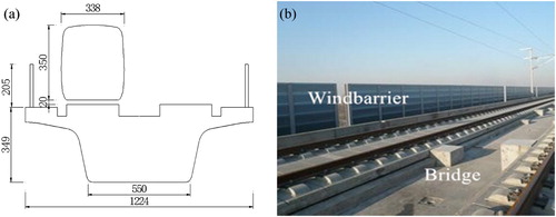
In this study, the bridge model is a 32 m double-line simple-supported beam-bridge. For the sake of simplicity, the bridge piers are ignored. In the present paper, the cases with the train on the windward track of bridge are analysed, because its aerodynamic stability issues are more profound relative to that on the leeward track (Guo et al., 2015). The wind barrier used in this study is 2.05 m in height (Xiang et al., 2012; Xiang et al., 2014) with a porous ratio of 0%. The total length of the wind barrier is 96 m, which is divided into three segments. Each segment is further divided into 16 sections (as shown in Figure 2) to study the variation of its wind load along the line. A simplified CRH2 HST model with three-car multiple units (leading car, middle car, and tail car) is used in the present study. The HST model is totally 76.4 m (25.7 + 25 + 25.7) long. The spacing between the train and the track slab is 0.2 m. The bogies are not considered for simplicity. The total length of the bridge is 352 m. The bridge is divided into eleven sections from left to right along its length. The wind barrier is located at 5#, 6#, and 7# sections, as shown in Figure 2(a). The computational domain and model details are presented in Figure 2 and Figure 3.

Figure 2. Simulation model: (a) schematic diagram of models; (b) computation domain and meshes.

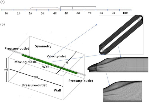
Figure 3. Vehicle-bridge system and wind barrier: (a) CAD of the model; (b) a practical bridge and wind barrier.

Unsteady incompressible N-S equations are used to solve the flow field for the cases with a train running on the bridge and pass by the wind barrier. A Shear Stress Transport (SST) turbulence model is widely used in numerical simulation of the flow around the train (Liang et al., 2020; Yao et al., 2020), which is designed to deal with adverse pressure gradients and separated flows (Menter et al., 2003). The SST k-ω turbulence model is used as the turbulence closure for the RANS equations listed below: (5) $\frac{\mathrm{\partial }}{\mathrm{\partial }\text{t}}(\rho \mathrm{k})+\frac{\mathrm{\partial }}{{\mathrm{\partial }}_{\text{xi}}}(\rho \mathrm{k}{\text{u}}_i)=\frac{\mathrm{\partial }}{{\mathrm{\partial }}_{xj}}\left({\mathrm{\Gamma }}_k\frac{\mathrm{\partial }k}{\mathrm{\partial }{\text{x}}_{\text{j}}}\right)+{\tilde{G}}_k-Y_k+S_k{G}_k.$(5) (6) $\begin{array}{rl}& \frac{\mathrm{\partial }}{\mathrm{\partial }\text{t}}(\rho \mathrm{w})+\frac{\mathrm{\partial }}{{\mathrm{\partial }}_{\text{xj}}}(\rho \mathrm{w}{\text{u}}_j)\\ & =\frac{\mathrm{\partial }}{{\mathrm{\partial }}_{xj}}\left({\mathrm{\Gamma }}_w\frac{\mathrm{\partial }w}{\mathrm{\partial }{\text{x}}_{\text{j}}}\right)+Gw-Y_w+D_w{S}_w.\end{array}$(6) where Γ_k and Γ_ω are the effective diffusivity of k and ω; Ğ_k represents the generation of turbulence kinetic energy due to the mean velocity gradients, calculated from G_k; G_ω is the generation of ω;Y_k and Y_ω are the dissipation of k and ω, respectively; D_ω is the cross-diffusion term; S_k and S_ω are user-defined source terms. Reynolds-averaged Naver-Stokes (RANS) equations were solved together with shear stress transport (SST) k-ω turbulence model (Menter, 1994), the constants in the turbulence model are α=1, α_ω=5/9, β_k = 0.09, β_ω = 0.09, σ_k=2, σ_ω = 2 and a₁=0.31. For the solution of the pressure and velocity coupling equation, the semi-implicit method for the pressure-linked equations (SIMPLE) algorithm was selected. Second-order upwind scheme discretizes the convection and diffusion terms, and the second-order implicit scheme discretizes the time derivative for unsteady flow calculations.

Moving mesh technology is used to realize the moving of the HST model. This technique allows the relative moving between adjacent grids, so the mesh surface does not need to be re-arranged on the interface. The computational domain consists of two subdomains: a stationary part that contains the bridge and infrastructures, the other is a moving part that contains the train. The boundary conditions and grid distribution are shown in the Figure 2(b).

Figure 4 shows the relative wind direction for a running train. U represents the oncoming cross-wind velocity, which is perpendicular to the bridge; V is the speed of the train, $U_H=\sqrt{{(U)}^2+{(V)}^2}$ is the actual wind speed acting on the train; and α is the effective yaw angle, which is $\alpha =\arcsin \frac{U}{U_H}$.

Figure 4. Resultant wind velocity and angle.

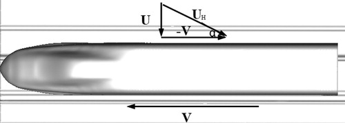
Two yaw angles of 8.87 and 90 degree represent two typical cases for train aerodynamics in cross-wind. The former one, i.e. 8.87 degree, represents the case with U = 15.0 m/s and V = 97.2 m/s (350 km/h), which corresponds to cases C1 and C1-b in Table 1. The later one, i.e. 90 degree, represents the case with U = 35.0 m/s and V = 0 m/s (the train stops on bridge), which corresponds to cases C3 and C3-b in Table 1. Note that, the cross-wind velocity U of 15 m/s is the upper limit for the normal operation of HSR. (TMRR, 2019).

Table 1. Different cases considered in numerical simulation.

Case	Wind barrier	Train statues (effective yaw angle)
C1	Uninstalled	Moving train (8.87^o)
C1-b	Installed
C2	Uninstalled	Stationary train (8.87^o)
C2-b	Installed
C3	Uninstalled	Stationary train (90^o)
C3-b	Installed

Moreover, another case usually used in traditional wind tunnel experiments is also simulated in the present paper, i.e. C2 and C2-b in Table 1. Although the yaw angle of the train is also 8.87 degree, which is achieved by yawing the train model, the train and bridge are both stationary and bear the same yaw angle. C2 and C2-b cases are used in the present paper to compare with C1 and C1-b to highlight the dilemma of wind tunnel experiments using stationary train models.

Additionally, Figure 6 of the manuscript reports the simulation results at different yaw angles and compares them with those in literatures. All these results of different yaw angles are achieved using moving train model scenario with different train speed V. These results in Figure 6 are used only for validating the present CFD simulation techniques. And only the cases listed in Table 1 are discussed in detail in the present paper.

3. Results and discussions

3.1. Grid independence and validation

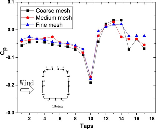
The computational domain is 30 B × 19 B × 10 B (B is the bridge width), together with its boundary conditions, as shown in Figure 2 (b). To verify the quality of mesh in this research, the cross-wind comparisons reported here, three sets of meshes are compared – the coarse mesh with 8 million cells, the medium mesh with 12 million cells, and the fine mesh with 18 million cells. Figure 5 indicates the results obtained from the three meshes. As shown in Figure 5, the Cp distribution is quite similar for the three meshes, especially on the windward, upper and leeward surfaces. However, Cp on the bottom of the train bears a significant difference for the three meshes. Since Cp on the bottom of the train is dominated by the gap flow between the train and bridge, it should be uniform with the bogies and track ignored. Moreover, the result obtained from the fine mesh is smoother and in a closer and more orderly array. The curve is fundamentally in conformity with the field test performance of the tendency (Liu et al., 2018). Therefore, the fine mesh is adopted in the following simulations. Grids near the bridge and train surface are defined as shown in Figure 2(b) to get a better resolution for the near-wall flow structures. The grid size near the train surface is 0.001 m, and the maximum size of the bridge and the wind barrier is 0.04 m and 0.02 m, respectively.

Figure 5. Measure points of the sections.

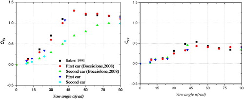
To validate the accuracy of the present numerical simulation, multiple forms of grid division were developed for investigations similar to the above mentioned, and then the comparison of results is presented in Figure 6. A lot of related studies show that the aerodynamic loads of the train only depend on the reference velocity of a train (U_H) as a result of the combination of wind speed U and train speed V. The effective yaw angle α is also changed with V as well. Based on this, Figure 6 compares the present C_Fx and C_Fz of the leading and middle carriages with those reported by Bocciolone et al. (2008) and Baker (1991). It is shown that the present simulation results fit quite well with that reported in the work of literature, with the maximal discrepancy less than 10%, suggesting that the present simulation results are reliable enough.

Figure 6. Experimental and computational results comparison.

3.2. Wind barrier effects on HST

3.2.1. Aerodynamic forces of a moving and stationary train model

A lot of wind tunnel and CFD investigations used stationary train models with different yaw angles to simulate the effective yaw angle caused by its moving in a cross-wind (Bocciolone et al., 2008; Niu et al., 2017; Suzuki et al., 2002). To reflect the relationship between the running train and bridge, the results using a moving model and a stationary model with the same effect yaw angle should be compared. Figure 7 presents the aerodynamic forces on the train when it passes through the wind barrier, as shown in Figure 2. The results using a moving train model (the curve line) and those using a stationary train model (the solid and dash straight lines) with the same effective yaw angle are compared in Figure 7. The solid and dash lines indicate the cases with and without wind barriers, respectively. The vertical green and red dash lines in Figure 7 indicate the time from the train head enters the wind barrier to the its end leaves the area, respectively.

Figure 7. Aerodynamic coefficients of train: (a) C_Fx; (b) C_Fz; (c) C_Mx.

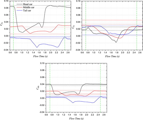
Before the train enters the wind barrier, the side force coefficient C_Fx of each car is quite stable, although different along the train. C_Fx is the largest for the leading car, which is about 0.082. It reduces to 0.024 for the middle car, and reduces to a small negative value for the tail car, as shown in Figure 7. This observation is qualitatively analogous to that reported by Liu and Zhang (2013) and Niu et al. (2018), suggesting the flow is quite three dimensional along the train when it is running in a cross-wind.

When the train enters the wind barrier, C_Fx of the head car reduces significantly to about 0.01 and then increases gradually as moving in the wind barrier region. Before the sudden recovery of C_Fx, which presences when the train leaves the wind barrier region, there is a small drop of C_Fx, when the train head approaches the end of the wind barrier. The reduction in C_Fx of the middle car is far less pronounce relative to that of the leading car. Besides, the C_Fx of the tailing car becomes more negative once it enters the wind barrier region. The sudden drop in C_Fx is apparently ascribed to the sheltering effect of the wind barrier, which provides a zone of negative pressure downstream (Avila-Sanchez et al., 2016).

The lift force coefficients C_Fz of the head car changes from slightly positive to negative, once the train enters the barrier region. It recovers quickly to its initial value when the head car leaves the barrier. The C_Fz of the middle car also changes from positive to negative and then recovers to its initial value during the whole process. On the other hand, C_Fz of the tailing car is always positive, although it also suffers a reduction and recovery process, as shown in Figure 7. Variation of momentum coefficient C_Mxis qualitatively similar to that of C_Fx and C_Fz.

When there is no wind barrier, the simulation results of C_Fx using a stationary model are quite similar to that of using a moving model. However, when the train is running downstream of the wind barrier, the C_Fx using a stationary model differs significantly from that using a moving model, especially for the leading and tailing cars, as illustrated in Figure 7. The difference in C_Fz and C_Mx between the stationary and moving model cases is more pronounced. For example, the C_Fz of the leading car changes from positive to negative when the train enters the wind barrier region, as shown in Figure 7. However, the C_Fz of the leading car is always positive, for the cases using a stationary train model.

These observations indicate that the method using a stationary train model may be applicable to the case when there is no wind barrier. Once the train is running downstream to a wind barrier, the relative motion, and slipstream caused by the moving of the train had significant effects on its aerodynamic forces. Thus, stationary model simplification is no longer applicable.

Figure 8 compares the side force on the bridge girder for the two simulation methods using the stationary model and moving models. The effect of wind barrier is also investigated. The horizontal lines are the simulation results with a stationary model. The red lines indicate the case with α = 8.87°, and the black lines are the cases with α = 90°. The solid and dot lines are the cases with and without wind barriers, respectively. The circle and star symbols are the moving model cases with and without wind barrier.

Figure 8. Comparison of the aerodynamics of bridge.

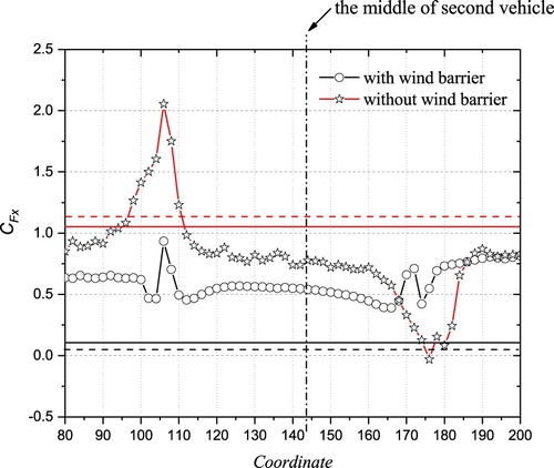
Obviously, in the cases with a stationary train model, the C_Fx of the bridge is constant since there is no relative movement between the train and the bridge. Although the presence of wind barrier has the opposite effect on the C_Fx of the bridge at α = 8.87° and 90°, the effect of wind barrier on the C_Fx of the bridge is quite limited for the stationary model cases, as shown in Figure 8. Another critical point is that, if the stationary model with α = 8.87° is used to simulate the moving train in a cross-wind, the bridge model will have the same yaw angle, although it is perpendicular to the oncoming flow in the real case. This scenario will significantly underestimate the C_Fx of the bridge, as shown in Figure 8.

For the moving model method, the effects of the oncoming flow and the relative motion can be adequately simulated. As shown in Figure 8, C_Fx of the bridge in moving model cases largely lies between the two stationary model cases. Especially for the case without the wind barrier, the C_Fx is quite similar to that in the stationary model case with α = 90°. More importantly, the moving model method can capture the impulsive effect of the train on the C_Fx of the bridge, especially for the case without the wind barrier. Particularly, the C_Fx of the bridge is more than doubled once the train approaches, which may influence the dynamic response of the bridge.

3.2.2. Pressure distribution on the train

Figure 9 shows the six cross-sections along the train where the pressure distribution is monitored. In each section, there are 17 pressure taps distributed circumferentially around the train. The wind pressure coefficient C_p is expressed as (7) $C_p=\frac{P-P_0}{0.5\rho {U^2}_H}.$(7) where P is the static pressure on the train surface; P₀is the reference atmospheric pressure; U_H is the reference velocity.

Figure 9. Pressure monitoring positions.

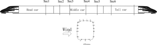
Figure 10 compares the pressure distribution along the train for the cases using a moving model, i.e. C1 and C1-b. Among all the monitored sections, the C_p distribution of Sec 1 and Sec 6 differs the most obvious from that in other sections, which are apparently caused by the strong three-dimensional effects near both ends of the train. For the case without wind barrier, i.e. C1, as shown in Figure 10(a), the pressure at the centre of the windward face is positive, except that near the tail of the train. For all test sections, the pressure at point 10, which is located near the up shoulder of the train, is the most negative. This observation suggests the flow separates near point 10. Contrarily, there is no significant negative pressure on the bottom surface, because the flow through the gap between the train and bridge is confined within a small area, and no strong flow separation occurs.

Figure 10. Pressure coefficient at different sections for the case using a moving model: (a) No wind barrier; (b) Wind barriers.

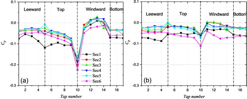
Once the train enters the wind barrier region, Figure 10 (b), the pressure distribution becomes quite different from that in the open area. First, the pressure on the windward face all becomes negative, which means the wind barrier provides a low-pressure region for the train downstream. Second, the intense negative pressure at the up shoulder of the train disappears, suggesting the wind barrier suppresses the flow separation on the train. Besides, the difference between the pressure on the windward and leeward faces becomes less pronounced relative to that in an open area.

Figure 11 presents the pressure distribution along the train using a stationary model with α of 8.87^o and 90^o. For cases without wind barriers, as shown in Figure 11(a). C_pof all test sections are negative except that on the windward face at α = 90^o. Except that on the bottom surface, the magnitude of C_p for the case with α = 90° is much larger than that for α = 8.87°. Apparently, this is because of the flow around the train transits from bluff body state at α = 90° to slender body state at α = 8.87° (Cheli, Corradi, et al., 2010).

Figure 11. Pressure coefficient at different sections for the case using a stationary model: (a) No wind barrier; (b) Wind barriers.

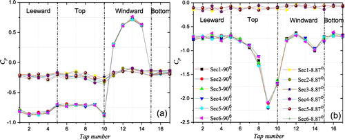
Moreover, by comparing the results shown in Figure 10 and Figure 11, it can be found that the C_p distribution is quite different for the case using a stationary model with α = 8.87° and the case using a moving model with the same effective yaw angle. This observation suggests that the method using a stationary model with the same yaw angle cannot fully reveal the aerodynamic characteristics of a train when it is running on a bridge. Because of the relative motion between the train and bridge may play an essential role in this case, which cannot be neglected.

3.3. Aerodynamic forces on the wind barrier

The aerodynamic forces on a wind barrier are crucial for its structural design. Moreover, the transient force on a wind barrier caused by the passing of HST may incur its fatigue failure. Obviously, the pulsing effect caused by a running train cannot be simulated if a stationary model is adopted. Figure 12 shows the lateral force on the middle section of the wind barrier, which is normalized using the cross-wind velocity. The red and the blue dashed lines represent the results using a stationary model with α of 8.87^o and 90^o, respectively.

Figure 12. Lateral force coefficient of wind barriers.

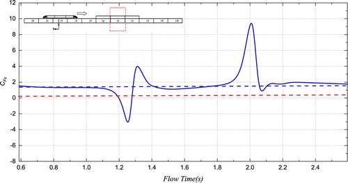
Apparently, the moving model method captures the impulsive effect of the lateral force on the wind barrier, which cannot be revealed by the stationary model, regardless of the yaw angel adopted. As expected, when the train is far from the wind barrier, the side force on the barrier C_Fx is about 1.7, equals to that of the stationary model method with α = 90^o. Once the train head approaches, C_Fx presents a sudden drop and reaches a minimum value of about -2.9. This observation suggests that the high-pressure region near the train head induces a side force on the barrier opposite to the cross-wind direction. With the train head passing by, the C_Fx on the barrier shoots up to a maximal value of about 4.0, which is far more significant than the lateral force caused by the cross-wind. After pulsing behavior mentioned above, the C_Fx returns approximately to its initial value and keeps almost unchanged when the train body passes by. Another pulsing jump of C_Fx presents when the train tail passes the barrier, which is much more pronounced than that caused by train head with the maximum C_Fx reaches approximately 9.2. This observation suggests that the low pressure in the trailing vortices of an HST has more significant effects on the surrounding structures.

3.4. Flow structures around the train and bridge

To identify the effects of the yaw angle on the flow structure around the HST and bridge, Figure 13 shows the instantaneous vortex structures near the HST and bridge for cases listed in Table 1. The instantaneous flow structures are revealed by the iso-surface of the second invariant of the velocity gradient Q, which is defined as $Q=-1/2\mathrm{\partial }{u}_{i,j}\mathrm{\partial }{u}_{i,j}$ and colored by the normalized streamwise velocity u.

Figure 13. Instantaneous iso-surface plot of Q-criteria collared by mean wind velocity U.

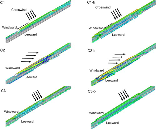
Figure 14. Flow structures in the central plane of the train and bridge.

For case C1 with a moving train model no wind barrier, there is a robust vortex detached from near the leeward side of the roof, which develops along the train. This vortex is similar to that downstream of the slender body, as reported by Khier et al. (2000). Besides, the other pair of counter-rotating trailing vortices occur at the tail of the train, which is skewed to the downstream direction apparently. Once the train is in the wind barrier region, all these vortices are suppressed and broken into small vortices. Generally, the shear layer from the wind barrier over shots the train, suppressing the trailing vortices.

There are significant differences among cases C1, C2 and C3, and the latter two are stationary mode cases with a yaw angle of 8.87^o and 90^o (see Table 1), respectively. In C2, the stationary mode case with the same yaw angle with C1, the detached vortex still presences at the leeward side of the train, although it is broader and shorter relative to that in C1. Moreover, the pair of deflective trailing vortices at the train tail in C1 disappears in C2, which is replaced by a single trailing vortex at the windward side near the tail. This observation suggests that even with the same yaw angle, a stationary train model cannot fully reproduce the flow structures around a running train, especially the trailing vortices in its near wake. For C3, the stationary model case with a yaw angle of 90^o, the above-mentioned trailing vortices in C1 disappear completely. The flow is dominated by the quasi-two-dimensional (2D) vortex formed at the roof of the train model, which is inherently similar to that downstream a 2D bluff body near a wall in cross-flow.

For the cases with the presence of wind barrier, the moving model case C1-b differs more significantly from the stationary cases C2-b and C3-b, as shown in Figure 13. In the real case, i.e. C1-b, the flow is perpendicular to the wind barrier, although the effective yaw angle of the moving train is 8.87°. The flow separates at the tip of the wind barrier, forming a low-speed region downstream. This low-speed region significantly weakens the trailing vortices at the train leeward and the symmetrical trailing vortices at the train tail as well, although they are still observable in C1-b.

For the C2-b case, both bridge, wind barrier, and the train had the same yaw angle of 8.87°. Apparently, strong trailing vortices are formed behind the wind barrier at its both end, which is significantly different from the real case, i.e. C1-b. Similarly, the C3-b case with the yaw angle of 90° also cannot reproduce the real flow structures observed in C1-b.

Moreover, in the comparison of these cases, when a train runs at high speed, the slipstream and trailing vortex caused by the train and bridge becomes longer and the vortex intensity increases. The slipstream of the train is immersed in the vortex shedding from the bridge, merges with the vortex structure it produces, and flows away. The impact of cross-wind on the main vortex region around the bridge gradually increases with increasing yaw angle. Also, when the train running in the wind barrier, the vortex structure becomes thicker, the vortex strength increases significantly, and the unsteadiness becomes more obvious. Furthermore, through these differences from the instantaneous iso-surface plot, the shedding vortex is intermittent and not continuous, the motion of vortexes and their position relation have some randomness when the train was running. These unsteady flow structures are the cause of unsteady aerodynamic forces.

Generally, for the case without wind barrier, despite the stationary mode with a yaw angle of 8.87° (C2) can mostly reproduce the primary vortex (i.e. trailing vortex) around the train, there are significant differences in the structure and strength of the flow around the train. That is, for the cases with and without a wind barrier, only the moving mode method (C1 and C1-b) can reproduce the real case.

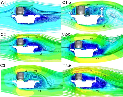
Figure 14 shows the flow structures in the central plane of the train and bridge for Case C1 to C3 with/without wind barrier (see Table 1). The streamline is used to reveal the flow structures, which is colored by the normalized streamwise velocity u.

For Case C1 with a moving train model running in an open area, there is a small vortex V1 on the windward side of the moving train, which disappears in the stationary model cases C2 and C3. The large-scale leading-edge vortex V2 presents at the leeward of the train. Besides, a vortex V3 is observed downstream of the bridge girder. When the train runs in the wind barrier region, the leading-edge vortex breaks into small-scale complex vortices at the train leeward, i.e. V7, V8, V9. Moreover, alternate vortex shedding occurs downstream of the bridge. This observation may be ascribed to the effects of the wind barrier, which makes the bridge ‘blunter’ in cross-flow.

For the two stationary model cases without wind barrier, i.e. C2 and C3, the leading-edge vortex separates into two vortices, i.e. V2 and V4, under the effects of the gap flow. Particularly, in C3 with the yaw angle of 90°, the gap flow is more significant than that in C2. This observation suggests that the relative motion between the train and bridge may suppress the gap flow. That is, experiment using the stationary model cannot fully reproduce the flow structures around a running train. For the cases with the presence of wind barrier, the moving model case C1-b differs more significantly from the stationary cases C2-b and C3-b, as shown in Figuer 14. In the moving model case C1-b, the flow between the two wind barriers contains complex small-scale vortices, i.e. V7, V8, and V9, which may be ascribed to the interaction between the separated flow from the barrier and the slipstream caused by the train. However, for the cases with a stationary model, C2-b, and C3-b, the flow structures are much different from that of the moving model case C1-b.

4. Concluding remarks

Using the computational fluid dynamic method, the present paper investigates the aerodynamic characteristics of a high-speed train on a bridge girder in cross-flow. The sheltering effects and wind load of wind barriers are compared for cases with running train models and stationary models. Both the aerodynamic load and flow around the model are compared in detail. The following conclusions can be drawn:

Despite the case using a stationary mode with the yaw angle of 8.87° (C2) can largely reproduce the primary vortex (i.e. trailing vortex) around the train, there are significant differences in the structure and strength of the flow. Furthermore, for cases with the train passing by a wind barrier region, the relative motion and slipstream caused by the moving train have significant effects on its aerodynamic forces. Thus, stationary model simplification is no longer applicable no matter what yaw angle adopted.

The aerodynamic forces on the train various along the train even it is running in a steady cross-flow, suggesting the flow around the train is highly three-dimensional along the train. These aerodynamic forces suffer significant and sudden reduction and recovery when the train enters and leaves a wind barrier region. This sudden variation in aerodynamic forces of the train is deleterious for its running stability. The lateral force on the wind barrier also bears remarkable pulsing behavior when the train enters and leaves the barrier region. The maximum pulsing amplitude between the positive and negative peaks is about 10 times larger than that caused by cross-wind. However, these unsteady pulsing behaviors of the aerodynamic forces on the train and wind barrier cannot be revealed using stationary model simplification regardless of the yaw angle adopted.

Due to the limitations of this study, a new moving model testing system has been constructed in the wind tunnel of Central South University. Moving model tests in cross-wind will be conducted to deepen our understanding of the unsteady pulsing behaviors of the aerodynamic forces for both the train and the wind barrier, which will enhance the operational safety for the HSR lines in windy areas.

Acknowledgment

The research described in this paper was financially supported by the National Natural Science Foundations of China (No. 51925808, U1934209) and the National Key R&D Program of China (No. 2017YFB1201204) and program of China Scholarships Council. Shanghai Key Lab of Vehicle Aerodynamics and Vehicle Thermal Management Systems (VATLAB-2018-01) is also acknowledged.

Disclosure statement

No potential conflict of interest was reported by the authors.

Additional information

Funding

This work was supported by ; National Natural Science Foundations of China: [Grant Number 51925808, U1934209]. Shanghai Key Lab of Vehicle Aerodynamics and Vehicle Thermal Management Systems (VATLAB-2018-01).

References

- Akbarian, E., Najafi, B., Jafari, M., Faizollahzadeh Ardabili, S., Shamshirband, S., & Chau, K.-W. (2018). Experimental and CFD-based numerical simulation of using natural gas in a dual-fuelled diesel engine. Engineering Applications of Computational Fluid Mechanics, 12(1), 517–534. https://doi.org/10.1080/19942060.2018.1472670
- Auvity, B., Bellenoue, M., & Kageyama, T. (2001). Experimental study of the unsteady aerodynamic field outside a tunnel during a train entry. Experiments in Fluids, 30(2), 221–228. https://doi.org/10.1007/s003480000159
- Avila-Sanchez, S., Lopez-Garcia, O., Cuerve, A., & Meseguer, J. (2016). Characterization of cross-flow above a railway bridge equipped with solid windbreaks. Engineering Structure, 126, 133–146. https://doi.org/10.1016/j.engstruct.2016.07.035
- Baker, C.J. (1991). Ground vehicles in high cross winds Part I: Steady aerodynamic forces. Journal of Fluid and Structures, 5(1), 69–90. https://doi.org/10.1016/0889-9746(91)80012-3
- Baker, C.J., Dalley, S.J., Johnson, T., Quinn, A., & Wright, N.G. 2001. The slipstream and wake of a high-speed train. Proceeding of the Institution of Mechanical Engineers, Part F: Journal of Rail and Rapid Transit, 215(2), 83–99. https://doi.org/10.1243/0954409011531422
- Baker, C.J., Quinn, A., Sima, M., Hoefener, L., & Licciardello, R. (2014a). Full-scale measurement and analysis of train slipstreams and wakes. Part 1 : Ensemble averages. Proceedings of the Institution of Mechanical Engineers, Part F: Journal of Rail Rapid Transit, 228(5), 451–467. https://doi.org/10.1177/0954409713485944
- Baker, C.J., Quinn, A., Sima, M., Hoefener, L., & Licciardello, R. (2014b). Full-scale measurement and analysis of train slipstreams and wakes. Part 2: Gust analysis. Proceedings of the Institution of Mechanical Engineers, Part F: Journal of Rail Rapid Transit, 228(5), 468–480. https://doi.org/10.1177/0954409713488098
- Bell, J.R., Burton, D., Thompson, M., Herbst, A., & Sheridan, J. (2014). Wind tunnel analysis of the slipstream and wake of a high-speed train. Journal of Wind Engineering and Industrial Aerodynamics, 134, 122–138. https://doi.org/10.1016/j.jweia.2014.09.004
- Bell, J.R., Burton, D., Thompson, M.C., Herbst, A.H., & Sheridan, J. (2015). Moving model analysis of the slipstream and wake of a high-speed train. Journal of Wind Engineering and Industrial Aerodynamics, 136, 127–137. https://doi.org/10.1016/j.jweia.2014.09.007
- Bocciolone, M., Cheli, F., Corradi, R., Muggiasca, S., & Tomasini, G. (2008). Cross-wind action on rail vehicles: Wind tunnel experimental analyses. Journal of Wind Engineering and Industrial Aerodynamics, 96, 584–610. https://doi.org/10.1016/j.jweia.2008.02.030
- Catanzaro, C., Cheli, F., Rocchi, D., Schito, P., & Tomasini, G. (2016). High-speed train cross-wind analysis: CFD study and validation with wind-tunnel tests. Lect. Notes Appl. Comput. Mech, 79, 99–112. https://doi.org/10.1007/978-3-319-20122-1_6
- Cheli, F., Corradi, R., Rcocchi, D., Tomasini, G., & Maestrini, E. (2010). Wind tunnel tests on train scale models to investigate the effect of infrastructure scenarios. Journal of Wind Engineering and Industrial Aerodynamics, 98(6-7), 353–362. https://doi.org/10.1016/j.jweia.2010.01.001
- Cooper, R.K. (1980). Probability of trains overturning in high winds. Wind Engineering, 1185–1194. https://doi.org/10.1016/B978-1-4832-8367-8.50109-1
- Ghalandari, M., Shamshirband, S., Mosavi, A., & Chau, K.-w. (2019). Flutter speed estimation using presented differential quadrature method formulation. Engineering Applications of Computational Fluid Mechanics, 13(1), 804–810. https://doi.org/10.1080/19942060.2019.1627676
- Guo, W.W., Wang, Y.J., Xia, H., & Lu, S. (2015). Wind tunnel test on aerodynamic effect of wind barriers on train-bridge system. Science China Technological Sciences, 58(2), 219–225. https://doi.org/10.1007/s11431-014-5675-1
- He, X.H., Shi, K., Wu, T., & Zhu, Y. (2016). Aerodynamic performance of a novel wind barrier for train-bridge system. Wind and Structures, 23(3), 171–189.
- He, X.H., Zhou, L., Chen, Z.W., Jing, H.Q., Zou, Y.F., & Wu, T. (2018). Effect of wind barriers on the flow field and aerodynamic forces of a train-bridge system. Proceeding of the Institution of Mechanical Engineers. Part F: Journal of Rail and Rapid Transit, 1–15. https://doi.org/10.1177/0954409718793220
- He, X.H., Zou, Y.F., Wang, H.F., Han, Y., & Shi, K. (2014). Aerodynamic characteristics of a trailing rail trains on viaduct based on still wind tunnel experiments. Journal of Wind Engineering and Industrial Aerodynamics, 2014(135), 22–33. https://doi.org/10.1016/j.jweia.2014.10.004
- Hemida, H., Baker, C., & Gao G, J. (2012). The calculation of train slipstreams using large-eddy simulation. Proceedings of the Institution of Mechanical Engineers. Part F: Journal of Rail and Rapid Transit, 228(1), 25–36. https://doi.org/10.1177/0954409712460982
- Huang, D.Y., Gao, W., & Kim, C.N. (2010). A numerical study of the train-induced unsteady airflow in a subway tunnel with natural ventilation ducts using the dynamic layering method. Journal of Hydrodynamics, 22(2), 164–172. https://doi.org/10.1016/S1001-6058(09)60042-1
- Huang, S., Hemida, H., & Yang M, Z. (2014). Numerical calculation of the slipstream generated by a CRH2 high-speed train. Proceedings of the Institution of Mechanical Engineers, Part F: Journal of Rail and Rapid Transit, 230(1), 103–116. https://doi.org/10.1177/0954409714528891
- Khier, W., Breuer, M., & Durst, F. (2000). Flow structure around trains under side wind conditions: A numerical study. Computers & Fluids, 29(2), 179–195. https://doi.org/10.1016/S0045-7930(99)00008-0
- Krajnović, S., Ringqvist, P., Nakade, K., & Basara, B. (2012). Large eddy simulation of the flow around a simplified train moving through a cross-wind flow. Journal of Wind Engineering and Industrial Aerodynamics, 110, 86–99. https://doi.org/10.1016/j.jweia.2012.07.001
- Liang, X.-F., Li, X.-B., Chen, G., Sun, B., Wang, Z., Xiong, X.-H., Yin, J., Tang, M.-Z., Li, X.-L., & Krajnović, S. (2020). On the aerodynamic loads when a high speed train passes under an overhead bridge. Journal of Wind Engineering and Industrial Aerodynamics, 202, 104–208. https://doi.org/10.1016/j.jweia.2020.104208
- Liu, T., Chen, Z., Zhou, X., & Zhang, J. (2018). A CFD analysis of the aerodynamics of a high-speed train passing through a windbreak transition under cross-wind. Engineering Applications of Computational Fluid Mechanics, 12(1), 137–151. https://doi.org/10.1080/19942060.2017.1360211
- Liu, T.H., & Zhang, J. (2013). Effect of landform on aerodyanmic performance of high-speed trains in cutting under cross-wind. Jounral of Central South University, 20(3), 830–836. https://doi.org/10.1007/s11771-013-1554-3
- Menter, F.R. (1994). Two-equation eddy-viscosity turbulence models for engineering application. AIAA Journal, 32(8), 1598–1605. https://doi.org/10.2514/3.12149
- Menter, F.R., Kuntz, M., & Langtry, R. (2003). Ten years of industrial experience with the SST turbulence model. Turbulence, Heat and Mass Transfer, 4, 625–632.
- Mou, B., He, B.-J., Zhao, D.-X., & Chau, K.-w. (2017). Numerical simulation of the effects of building dimensional variation on wind pressure distribution. Engineering Applications of Computational Fluid Mechanics, 11(1), 293–309. https://doi.org/10.1080/19942060.2017.1281845
- Muld, T.W., Efraimsson, G., & Henningson, D.S. (2012). Flow structures around a high-speed train extracted using Proper Orthogonal Decomposition and Dynamic Mode Decomposition. Computers & Fluids, 57, 87–97. https://doi.org/10.1016/j.compfluid.2011.12.012
- Niu, J.Q., Zhou, D., & Liang, X.F. (2017). Numerical simulation of the effects of obstacle deflectors on the aerodynamic performance of stationary high-speed trains at two yaw angles. Proceedings of the Institution of Mechanical Engineers, Part F: Journal of Rail and Rapid Transit, 1–15. https://doi.org/10.1177/0954409717701786
- Niu, J.Q., Zhou, D., & Liang, X.F. (2018). Numerical investigation of the aerodynamic characteristics of high-speed trains of different lengths under cross-wind with or without windbreaks. Engineering Applications of Computational Fluid Mechanics, 12(1), 195–215. https://doi.org/10.1080/19942060.2017.1390786
- Premoli, A., Rocchi, D., Schito, P., & Tomasini, G. (2016). Comparison between steady and moving railway vehicles subjected to crosswind by CFD analysis. Journal of Wind Engineering and Industrial Aerodynamics, 156, 29–40.
- Suzuki, M., Tanemoto, K., & Maeda, T. (2002). Aerodynamic characteristics of train/vehicles under cross winds. Journal of Wind Engineering and Industrial Aerodynamics, 91(1-2), 209–218. https://doi.org/10.1016/S0167-6105(02)00346-X
- TMRR. (2019). Technical management regulations for railway - high speed railway- Chapter 17: Driving in disaster weather. CR.
- Tomasini, G., Giappino, S., Cheli, F., & Chito, P. (2015). Windbreaks for railway lines: Wind tunnel experimental test. Journal of Rail and Rapid Transit, 0(0), 1–13. https://doi.org/10.1177/0954409715596191
- Wang, S., Bell, J.R., Burton, D., Herbst, A.H., Sheridan, J., & Thompson, M.C. (2017). The performance of different turbulence models (URANS, SAS and DES) for predicting high-speed train slipstream. Journal of Wind Engineering and Industrial Aerodynamics, 165, 46–57. https://doi.org/10.1016/j.jweia.2017.03.001
- Wang, M., Li, X.Z., Xiao, J., Zou, Q.Y., & Sha, H.Q. (2018). An experimental analysis of the aerodynamic characteristics of a high-speed train on a bridge under cross-winds. Journal of Wind Engineering and Industrial Aerodynamics, 177, 92–100. https://doi.org/10.1016/j.jweia.2018.03.021
- Xia, C., Shan, X.Z., & Yang, Z.G. (2016). Comparison of different ground simulation systems on the flow around a high-speed train. Proceedings of the Institution of Mechanical Engineers. Part F: Journal of Rail and Rapid Transit, 231(2), 135–147. https://doi.org/10.1177/0954409715626191
- Xia, C., Wang, H.F., Bao, D., & Yang, Z.G. (2018). Unsteady flow structures in the wake of a high-speed train. Experimental Thermal and Fluid Science, 98, 381–396. https://doi.org/10.1016/j.expthermflusci.2018.06.010
- Xia, C., Wang, H., Shan, X., Yang, Z., & Li, Q. (2017). Effects of ground configurations on the slipstream and near wake of a high-speed train. Journal of Wind Engineering and Industrial Aerodynamics, 168, 177–189. https://doi.org/10.1016/j.jweia.2017.06.005
- Xiang, C.Q., Guo, W.H., & Zhang, J.W. (2014). Numerical study on the optimal height of wind barriers and mechanism on high-speed railway bridge with double lines. Journal of Central South University (Science and Technology, 45(8), 2891–2898.
- Xiang, H.Y., Li, Y.L., & Liao, H.L. (2012). DEA-based evaluation of wind shielding effect of wind barrier for railway bridges. Journal of Southwest Jiaotong University, 47(4), 546–566.
- Xue, P., You, S.J., Cao, J.Y., & Ye, T.Z. (2014). Numerical investigation of unsteady airflow in subway influenced by piston effect based on dynamic mesh. Tunnelling and Underground Space Technology, 40, 174–181. https://doi.org/10.1016/j.tust.2013.10.004
- Yao, Z.Y., Zhang, N., Chen, X.Z., Zhang, C., Xia, H., & Li, X.Z. (2020). The effect of moving train on the aerodynamic performances of train-bridge system with a cross-wind. Engineering Applications of Computational Fluid Mechanics, 14(1), 222–235. https://doi.org/10.1080/19942060.2019.1704886
- Zhang, T., Guo, W.W., & Du, F. (2017). Effect of windproof barrier on aerodynamic performance of vehicle-bridge system. Procedia Engineering, 199(2017), 3083–3090. https://doi.org/10.1016/j.proeng.2017.09.426