Turbulence–chemistry interaction models with finite-rate chemistry and compressibility correction for simulation of supersonic turbulent combustion

Abstract

The turbulence–chemistry interaction model with finite-rate chemistry is a common model for solving supersonic turbulent combustion and takes into consideration the interaction between turbulent mixing and chemical reactions as well as finite chemistry reaction instead of the fast chemistry assumption. However, not only the density and viscosity but also the chemical reactions are affected by the compressibility of the flow field with an increasing Mach number. Considering engineering applications, the compressibility correction was introduced to two recent turbulence–chemistry interaction models with finite-rate chemistry, the Partially Stirred Reactor (PaSR) model and Unsteady PaSR (UPaSR) model, in a Reynolds-averaged Navier–Stokes framework. Numerical simulations of two typical supersonic combustors showed that the interaction between the turbulence and combustion was intensive within complex supersonic chemical reaction flow and could be described by the fine-scale structure volume fraction. The distributions of temperature, pressure, velocity and components somewhat downstream of fuel injection areas were most obviously improved by the presented models. Moreover, the increase in computational time consumption by the compressibility correction was less than 2%. It was found that the Compressible PaSR (C-PaSR) model and the UPaSR model show better consistency with experimental results than the traditional PaSR model.

KEYWORDS:

• Supersonic turbulent combustion
• chemical reaction
• PaSR model
• compressibility correction

1. Introduction

Turbulent combustion simulation has been widely used because of technical progress and plays significant roles in the fields of aeronautics, land and marine internal combustion engines, and air-breathing engines (Akbarian et al., 2018; Gonzalez-Juez et al., 2017). However, with increasing Mach and Reynolds numbers in a combustor, interaction between turbulent mixing and chemical reactions intensifies significantly. How to simulate this kind of combustion accurately and rapidly has become an urgent problem needing to be resolved.

Conventional finite-rate chemistry Reynolds-Averaged Navier–Stokes (RANS)-based simulations or Large Eddy Simulation (LES) simulations are inaccurate in simulating chemical reactions, because the averaged (filtered) chemical reaction rate calculated directly by averaged (filtered) parameters can be affected by its strong nonlinearity. In addition, combustion in scramjets with working Mach numbers beyond 5 is affected by complex phenomena like ignition and extinction. And the Damköhler number is close 1.0 because the magnitudes of the chemical reaction time and turbulence time are on the same scale. Under these conditions, traditional combustion models based on the fast chemistry assumption and equilibrium approximation, like the Eddy Break-Up (EBU) model, become inappropriate. So methods based on turbulence–chemistry interaction have been developed.

Hitherto, the accepted turbulence–chemistry interaction models were: (1) Flamelet Progress Variable (FPV) models (Williams, 2000), in which the reactions are assumed to take place in thin layers wrinkled by turbulence; (2) Conditional Moment Closure (CMC) models (Bilger, 1993; Klimenko, 1990), in which the species equations are conditionally averaged on some variables (like mixture fraction) to reduce the nonlinearity; (3) Linear Eddy Models (LEM) (Wirth & Peters, 1992), solving species equations and physical processes from a 1D perspective with full resolution; (4) Probability Density Function (PDF) models (Safer et al., 2010), employing presumed or transported probability density functions to model the filtered reaction rates; (5) Finite-rate Chemistry models, including the Thickened Flame Model (TFM) (Charlette et al., 2002),the Eddy Dissipation Concept (EDC) model (Magnussen, 1981), and the Partially Stirred Reactor (PaSR) model (Berglund et al., 2010); etc. All these models have their own respective advantages in particular conditions. However, with increasing Mach number, not only density and viscosity but also chemical reactions are affected by the compressibility of the flow field since it can accelerate reaction rate via increasing the collision frequency of molecules and changing the flame configuration, which in turn affects the combustion mode. Several researchers have studied compressibility in turbulence–chemistry interaction models. Saghafian (Saghafian et al., 2014, 2015) rescaled the source term of the progress variable in FPV models with temperature and density to account for perturbations caused by compressibility. And simulations of an a-priori study and the HIFiRE scramjet showed good agreement with experimental data. Zhao (Zhao et al., 2015) tabulated the flamelet database at a reference pressure and obtained quantities of other pressures by using a sixth-order polynomial of the reference pressure, which avoided expensive computation. Ingenito (Ingenito & Bruno, 2008, 2009, 2010; Ingenito et al., 2006a, 2006b) focused on the chemical reaction source term and proposed Ingenito Supersonic Combustion Modeling (ISCM), which was valuable to extend.

In this study, a new method is presented to simulate supersonic turbulent combustion by importing the compressibility correction into turbulence–chemistry interaction models with finite-rate chemistry. First, the Partially Stirred Reactor (PaSR) (Sabelnikov & Fureby, 2011) and Unsteady PaSR (UPaSR) (Moule et al., 2014) models are employed to simulate high Mach number turbulent combustion. Then, Ingenito’s compressibility correction theory (Ingenito & Bruno, 2010) is modified in a RANS framework and integrated into the PaSR and UPaSR models to propose the Compressible PaSR (C-PaSR) and Compressible UPaSR (C-UPaSR) models. After that, detailed comparisons between experiments and numerical simulations of two combustors using the hydrogen-fueled scramjet of the German Aerospace Center (DLR) and the direct-connected scramjet of NASA Langley Center (SCHOLAR) are carried out. The flow field, the interaction between turbulent mixing and chemical reactions, and the effects of compressibility on supersonic combustion are analyzed.

2. Theory description

2.1. Chemical source term closure method in finite-rate chemistry theory and EDC closure

Quasi-laminar combustion theory is a common method to deal with high-speed (supersonic) combustion, which ignores the influences of temperature and component fluctuation on combustion. So the chemical reaction rate can be represented using $\overline{{\dot{\omega }}_i}={\dot{\omega }}_i(\tilde{T},\tilde{\mathit{Y}})$. However, fluctuation plays a significant role in the heat dissipation within mixing layers and may lead to the self-ignition phenomenon (Moule et al., 2011). Hence, the interaction between turbulence and combustion needs to be taken into account when simulating supersonic turbulent combustion.

The EDC closure concept offers a basis for incorporating such inhomogeneities. It was originally proposed by and built on the early ED model (Magnussen & Mjertager, 1976), turbulent energy cascade theory, and highly discontinuous characteristics of the flow (Magnussen, 1981, 2005). Based on the theory of finite-rate chemistry and the EDC model, the basic units of the fluid are divided into fine-scale structures (denoted by the superscript *) and surrounding structures (denoted by the superscript ⁰) (Petrova, 2015). In detailed chemical simulations, a fine-scale structure region is regarded as a well-stirred reactor – called a Perfectly Stirred Reactor (PSR) – since the reaction rate is quite high due to the favourable mixing of the final products of fresh reactants. On the contrary, the reaction rate in surrounding structures is very low and can be neglected (Karrholm, 2008). From a general point of view, the mean chemical reaction rate can be expressed as (Girimaji, 1991; Moule et al., 2011) (1) $\overline{{\dot{\omega }}_i}={\int }_{\psi }P\left(\psi \right){\dot{\omega }}_F\left(\psi \right)d\psi$(1) where $P$ denotes the joint scalar Probability Density Function (PDF), $\psi =[T,\mathit{Y}{]}^{\text{T}}$ is the composition vector (temperature and species mass fraction) and $\psi$ is the associated domain of definition of the PDF. According to analyses in the literature (Moule et al., 2014), the PDF is assumed to be bimodal, which is decomposed into a fine-scale structures contribution and a surroundings contribution, $P\left(\psi \right)={\gamma }^{\ast }\delta (\psi -{\psi }^{\ast })+(1-{\gamma }^{\ast })\delta (\psi -{\psi }^0)$, so the mean chemical reaction rate becomes (2) $\overline{{\dot{\omega }}_i}={\gamma }^{\ast }{\dot{\omega }}_i\left({\psi }^{\ast }\right)+(1-{\gamma }^{\ast }){\dot{\omega }}_i\left({\psi }^0\right)$(2) where ${\gamma }^{\ast }$ denotes the fine-scale structure volume fraction, namely the fraction of the volume in which reaction processes take place. Assuming the second term to be zero, the chemical source term can be written as (3) $\overline{{\dot{\omega }}_i}={\gamma }^{\ast }{\dot{\omega }}_i\left({\psi }^{\ast }\right)$(3) The fine-scale structure volume fraction ${\gamma }^{\ast }$ is a crucial parameter in finite-rate chemistry models. The EDC model assumes that fine-scale structure is confined to the region with quasi-steady energy, where the turbulent kinetic energy is denoted by $k$. Assuming the turbulence is approximately isotropic, the volume fraction of the fine-scale structure is written as (4) ${\gamma }^{\ast }\approx 9.7{\left(\frac{\nu ϵ}{k^2}\right)}^{3/4}$(4) where $\nu$ is the viscosity coefficient and the dissipation rate$ϵ=({\upsilon }^{\mathrm{\prime }}{)}^3/\mathrm{\Delta }$, where ${\upsilon }^{\mathrm{\prime }}$and $\mathrm{\Delta }$ are the velocity fluctuation and the grid characteristic length, respectively. The mixing time-scale of the two regions is ${\tau }_m=0.41(\nu /ϵ{)}^{1/2}$.

2.2. PaSR model

The main difference between the PaSR model and EDC model is the simulation method for the fine-scale structure volume fraction ${\gamma }^{\ast }$ and the mixing time-scale ${\tau }_m$. The former combines the Kolmogorov time-scale and the chemical reaction time-scale, generally adopting the formula proposed by Sabelnikov and Fureby (Sabelnikov & Fureby, 2012, 2013): (5) ${\gamma }^{\ast }=\frac{{\tau }_{ch}}{{\tau }_{ch}+{\tau }_m}$(5) wherein the mixing time-scale ${\tau }_m$ is the harmonic mean value of the Kolmogorov time-scale ${\tau }_K$ and the grid time-scale ${\tau }_{\mathrm{\Delta }}$. In a mathematical description, it is ${\tau }_m=\sqrt{{\tau }_K{\tau }_{\mathrm{\Delta }}}$, where ${\tau }_{\mathrm{\Delta }}=\mathrm{\Delta }/{\upsilon }^{\mathrm{\prime }}$, ${\tau }_K=\sqrt{\nu /ϵ}$ and $ϵ=({\upsilon }^{\mathrm{\prime }}{)}^3/\mathrm{\Delta }$. And the chemical reaction time-scale ${\tau }_{ch}$ can be deduced from the approximation of a laminar premixed flame, that is ${\tau }_{ch}\approx {\delta }_u/S_u\approx \nu /S_u^2$, where ${\delta }_u$ and $S_u$ are the premixed flame thickness and the propagation velocity, respectively. The flame propagation velocity is based on a one-dimensional conservation law and the chemical kinetics (Turns, 2012). So ${\gamma }^{\ast }$ can be expressed as (6) ${\gamma }^{\ast }=\frac{{\tau }_{ch}}{({\tau }_{ch}+{\tau }_m)}=\frac{{\nu }^{3/4}{{\upsilon }^{\mathrm{\prime }}}^{5/4}}{S_u^2{\mathrm{\Delta }}^{3/4}+{\nu }^{3/4}{{\upsilon }^{\mathrm{\prime }}}^{5/4}}$(6) Since a small-scale grid is adopted in the LES framework by Sabelnikov, the above formulas can obtain fine results. If RANS and coarser grids are considered in this study, the dissipation rate is written as $ϵ=0.09k\omega$ to reduce the impact of the grid scale. Although the chemical time-scale based on a laminar premixed flame is chosen for the sake of simplicity in many options, Moule (Moule et al., 2011) mentioned in early analyses that the characteristic chemical time-scale that could be obtained from a diffusion flame at the limit of extinction was itself similar to the present estimate. This peculiar time-scale might therefore be suitable for both diffusion and premixed flames. Furthermore, iterative attempts reveal that the mixing time-scale shows a crucial influence on the fine-scale structure volume fraction.

It is necessary to use a composition vector of the fine-scale structure ${\psi }^{\ast }=[T^{\ast },{\mathit{Y}}^{\ast }{]}^{\text{T}}$ to calculate the chemical reaction source term ${\dot{\omega }}_i\left({\psi }^{\ast }\right)$, where $T^{\ast }$ and ${\mathit{Y}}^{\ast }=(Y_1^{\ast },\cdots Y_n^{\ast })$ are the temperature and mass fraction vector, respectively. For most combustion regions, the composition vector of fine-scale structure shows little contrast with its average value (Baudoin et al., 2009; Berglund et al., 2010; Huang et al., 2015); then the source term is commonly substituted by the latter, i.e. ${\dot{\omega }}_i(T^{\ast },{\mathit{Y}}^{\ast })\approx {\dot{\omega }}_i(\tilde{T},\tilde{\mathit{Y}})$. Under these conditions, the mean chemical reaction rate can be expressed as (7) $\overline{{\dot{\omega }}_i}\approx {\gamma }^{\ast }{\dot{\omega }}_i(\tilde{T},\tilde{\mathit{Y}})$(7)

2.3. Unsteady PaSR (UPaSR) model

Formula (6) shows that the modification of the chemical reaction source term by using the above PaSR model is attenuated, i.e. the flow inhibits chemical reactions when the time-scales of turbulence and chemical reaction are equivalent. For most combustion regions, this phenomenon is reasonable. It can explain extinction in simulation but is helpless to explain the self-ignition phenomenon. Moule (Moule et al., 2011) mentions that the temperature and mass fraction of the fine-scale structure in self-ignition regions vary greatly compared with their mean values, which leads to a large increase in ${\dot{\omega }}_i\left({\psi }^{\ast }\right)$. At this moment, the chemical reaction rate still increases when it is multiplied by the fine-scale structure volume fraction ${\gamma }^{\ast }$, and finally ignition occurs. Therefore, a more accurate method to simulate the chemical reaction source term should be adopted to reveal the complex turbulence–chemistry interaction.

Sabelnikov and Fureby (Sabelnikov & Fureby, 2011, 2013) reported the balance of species and energy between the fine-scale structures and the surrounding structures on the basis of LES, and proposed an Extended PaSR (EPaSR) model. Then, an Unsteady PaSR (UPaSR) model (Moule et al., 2014) was deduced from the EPaSR model by: (1) neglecting the convective terms in species conservation equations that describe the evolution of fine-scale regions; (2) instead of considering the differential equation for the fine-scale structure volume fraction ${\gamma }^{\ast }$, the mixing time-scale is assumed to be rather small so that ${\gamma }^{\ast }$ reaches its equilibrium value ${\gamma }_{eq}^{\ast }={\gamma }^{\ast }={\tau }_m/({\tau }_{ch}+{\tau }_m)$. After that, the UPaSR equations are given by (8) $\begin{array}{rl}& \frac{\mathrm{\partial }\overline{\rho }{Y}_k^{\ast }}{\mathrm{\partial }t}+\frac{\overline{\rho }}{{\tau }_m}\left(Y_k^{\ast }-Y_k^0\right)={\dot{\omega }}_k\left(T^{\ast },{\mathit{Y}}^{\ast }\right)\end{array}$(8) (9) $\begin{array}{rl}& \frac{\mathrm{\partial }\overline{\rho }{h}^{\ast }}{\mathrm{\partial }t}+\frac{\overline{\rho }}{{\tau }_m}\sum _{k=1}^N\left(Y_k^{\ast }{h}_k^{\ast }\left(T^{\ast }\right)-Y_k^0{h}_k^0\right)\\ & =\sum _{k=1}^N{h}_{k,f}^{\theta }{\dot{\omega }}_k\left(T^{\ast },{\mathit{Y}}^{\ast }\right)\end{array}$(9) where $k=1,2,\dots ,n$ represents the species number; $\rho$ is the density; and $h_{k,f}^{\theta }$ are the species formation enthalpies. Considering the relationship between variables in the two regions ${\overline{\psi }}_i={\gamma }^{\ast }{\psi }^{\ast }+(1-{\gamma }^{\ast }){\psi }^0$, the equations can be written as (10) $\begin{array}{rl}& \frac{\mathrm{\partial }\overline{\rho }{Y}_k^{\ast }}{\mathrm{\partial }t}+\frac{\overline{\rho }}{{\tau }_m\left(1-{\gamma }^{\ast }\right)}\left(Y_k^{\ast }-\widetilde{Y_k}\right)={\dot{\omega }}_k\left(T^{\ast },{\mathit{Y}}^{\ast }\right)\end{array}$(10) (11) $\begin{array}{rl}& \frac{\mathrm{\partial }\overline{\rho }{h}^{\ast }}{\mathrm{\partial }t}+\frac{\overline{\rho }}{{\tau }_m\left(1-{\gamma }^{\ast }\right)}\sum _{k=1}^N\left(Y_k^{\ast }{h}_k^{\ast }\left(T^{\ast }\right)-\widetilde{Y_k}{\tilde{h}}_k\left(\tilde{T}\right)\right)\\ & =\sum _{k=1}^N{h}_{k,f}^{\theta }{\dot{\omega }}_k\left(T^{\ast },{\mathit{Y}}^{\ast }\right)\end{array}$(11) When solving the equations, the initial conditions are from the mean parameters in the current timestep. The surrounding structure parameters can be calculated from the equation ${\psi }^0=(\tilde{\psi }-{\gamma }^{\ast }{\psi }^{\ast })/(1-{\gamma }^{\ast })$, where the fine-scale structure volume fraction ${\gamma }^{\ast }$ and the turbulent mixing time-scale ${\tau }_m$ are the same as those in the PaSR model.

Compared with the EPaSR model, the UPaSR model only needs to solve a set of ordinary differential equations to obtain fine-scale structure parameters for modifying the chemical reaction source term. Hence, this model can ensure a smaller amount of computational cost when considering the turbulence–chemistry interaction, which means it is more efficient in engineering applications.

2.4. The compressible modified PaSR model and the UPaSR model

When the velocity in a combustor is high or supersonic, not only flow but also combustion is affected by compressibility. Ingenito elaborates the effect of compressibility on supersonic turbulent combustion through perennial research. This research is divided into three parts (Ingenito & Bruno, 2008, 2009, 2010; Ingenito et al., 2006a, 2006b): (1) chemical reaction rate is affected by the local Mach number; (2) vorticity is mainly streamwise, and its creation and transport are driven also by baroclinic and dilatational terms; (3) the fine-scale structure region of combustion is approximately constant volume. On the basis of this research, the ISCM model is proposed.

Specifically, the first part introduces a modification of the molecular collision frequency (i.e. the reaction rate) by compressibility, which it describes in several forms (Ingenito & Bruno, 2008, 2010; Ingenito et al., 2006a, 2006b). One classical representative is $[1+M{a}^2]\dot{\omega }$. The second part corrects the subgrid kinetic energy $k_{SGS}$ when calculating the turbulent viscosity. In detail, $k^{\ast }$ is obtained from the turbulent energy equation of fine-scale structures, which leads to a new turbulent kinetic energy ${\overline{k}}_N={\gamma }^{\ast }{k}^{\ast }+(1-{\gamma }^{\ast })\overline{k}$. So the modified subgrid turbulent kinetic energy is $k_{SGS}={\overline{k}}_N-\overline{k}={\gamma }^{\ast }(k^{\ast }-\overline{k})$ and the turbulent viscosity is ${\mu }_t=\overline{\rho }\cdot \mathrm{\Delta }\cdot {\gamma }^{\ast }(k^{\ast }-\overline{k})$. 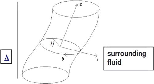The third part introduces the influence of compressibility on combustion regimes. In addition, the mechanism of this research is familiar with finite-rate combustion models based on fine-scale structure. Fine-scale structures of the ISCM model are considered to be perfect stirred reactors of tubular shape, as shown in Figure 1, where $\eta$ represents the characteristic turbulence length calculated by the Kolmogorov assumption and $\mathrm{\Delta }$ is the cell dimension. The volume fraction of the fine-scale structure adopted by Ingenito is ${\gamma }^{\ast }=\left(\pi {\eta }^2\mathrm{\Delta }\right)/{\mathrm{\Delta }}^3=\left(\pi {\eta }^2\right)/{\mathrm{\Delta }}^2$ (Ingenito & Bruno, 2008, 2009, 2010; Ingenito et al., 2006a, 2006b).

Figure 1. Reactor scheme in the fine-scale structure.

In this study, only the first and third parts are adopted when importing the compressibility correction, so only the chemical reaction rate needs to be revised (Ingenito & Bruno, 2010): (12) $\overline{\dot{\omega }}={\gamma }^{\ast }[1+2{\text{Ma}}_s^2]{\dot{\omega }}^{\ast }(T^{\ast },{\mathit{Y}}^{\ast })$(12) where $\text{M}{\text{a}}_s$ is the product of local turbulence intensity and the Mach number. In the simulations presented in Section 3, the turbulence intensity is of order of 10%. The volume fraction of the fine-scale structure is the same as that in the PaSR model ${\gamma }^{\ast }={\tau }_{ch}/({\tau }_{ch}+{\tau }_m)$. Ultimately, using the averaged composition vector for the chemical reaction source term would result in the Compressible PaSR model (the C-PaSR model); and if the source term of fine-scale structures is calculated by the UPaSR model, the new model is called the Compressible UPaSR (C-UPaSR) model.

3. Model description and numerical method

3.1. DLR combustor

The hydrogen-fueled scramjet of the German Aerospace Center (DLR) is a classical model to test the supersonic turbulence–chemistry interaction phenomenon. Oevermann’s (Oevermann, 2000) numerical simulation with a flamelet model showed good consistency with the experimental results. Génin (Génin et al., 2003) first used LES to simulate the combustor with the Linear Eddy Model (LEM). It was shown that the LES results were more reasonable and practical than those using RANS, especially for the far-field temperature distribution. After that, Berglund (Berglund & Fureby, 2007) used two kinds of flamelet model to analyze experimental and numerical schlieren images qualitatively. Fureby (Fureby et al., 2014) indicated that the PaSR model was more accurate than the two-equation flamelet model, especially for the prediction of temperature.

Figure 2 shows a schematic of the DLR supersonic combustor configuration (Oevermann, 2000), which is 300 mm in length with an inlet of 50 mm × 40 mm. The wedge-shaped strut (32 mm length × 6 mm height) has 15 uniformly-distributed injectors at the base with 1 mm diameter hydrogen injection. The origin of the coordinate system is 35 mm above the strut on the lower wall of the combustor. The upper wall has a diverging angle of 3° from the position at x = 58 mm. Because all injectors are at equivalent distances from each other in the transverse direction, only one is simulated with symmetrical boundary conditions (Berglund & Fureby, 2007; Fureby et al., 2014; Huang et al., 2015). In total, 3.18 million hexahedral meshes are generated, which are mainly clustered towards the upper, lower and strut walls, as well as its wake and shear layer regions. The grid topology around the strut and injector is displayed in Figure 3. The wall function is used for near-wall treatment.

Figure 2. Schematic of the DLR supersonic combustor configuration.

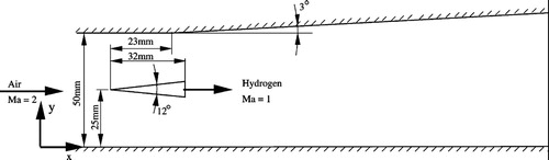
Figure 3. Grid topology near the injector (left) and symmetry of the strut (right).

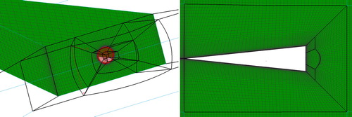
Table 1 shows the inflow parameters of the air inflow and hydrogen fuel. And the turbulent intensities are 0.5% and 5%, respectively. Because of the high Reynolds number in this model, the upper and lower walls are regarded as adiabatic sliding walls so as to be able to ignore the influence of the boundary layer on the central flow field and to reduce simulation consumption (Génin & Menon, 2010). Adiabatic and non-slip boundary conditions are adopted for the wall of the strut, and a first-order extrapolation boundary condition is employed for the outlet.

Table 1. Inflow conditions of the DLR model.

	Ma	V (m/s)	T (K)	P (atm)	$\rho$ (kg/m^3)	${\mathit{Y}}_{{\text{O}}_2}$	${\mathit{Y}}_{{\text{N}}_2}$	${\mathit{Y}}_{{\text{H}}_2\text{O}}$	${\mathit{Y}}_{{\text{H}}_2}$
Air	2.0	730	340	1.0	1.002	0.232	0.736	0.032	0
Jet	1.0	1200	250	1.0	0.098	0	0	0	1.0

3.2. The SCHOLAR combustor

The SCHOLAR model is an abbreviation for the direct-connected scramjet engine (Cutler et al., 2003; O’Byrne et al., 2004) developed by NASA Langley Research and Development Center. This model aims to generate a set of experimental data for testing the reliability of supersonic chemical reaction CFD codes and has been verified by various software. Rodriguez and Cutler used VULCAN to simulate this model (Rodriguez & Cutler, 2003). Their results showed the general flow structures were in good agreement with the experimental data. However, the wall pressure distribution, ignition location and penetration depth of the low-temperature zone in the center of the flame were difficult to make simultaneously consistent with the experimental results. In the work of Rodriguez and Cutler (2005), the influence of the inflow turbulent intensity, turbulent-to-laminar viscosity-ratio (${\mu }_T/{\mu }_L$), wall temperature, inflow components, turbulent Prandt number and Schmidt number were investigated. Cocks et al. (2011) investigated the influence of the turbulence–chemistry interaction (with an assumed PDF model and RANS) with PULSAR, which found that the correction was not significant. Then Cocks et al. (2012) used the hybrid RANS/LES method on finer grids and analyzed the evolution of a large number of vortex structures. Although the idea was heuristic, the results for the pressure and temperature fields were quite different from those from experiments.

Figure 4 shows the geometry of the SCHOLAR model, which is symmetric about the Z = 0 plane (perpendicular to the page) and has the width 87.88 mm. The design Mach number of the laval tube is 2.0. The equal cross-section isolator is 122.4 mm in length and 38.56 mm in height. Five small injectors on the upper surface of the isolator are neglected for simplification. The expansion part is 4.78 mm high and the combustor is 44.2 mm long. Starting from the position of hydrogen nozzle, the upper surface gradually expands to exit at 3°. The angle between the nozzle inflow and the combustor field is 30°, and the fuel injecting Mach number is 2.5. Two computational grids (with 2.7 and 6.6 million cells) are generated to verify the grid independence and choose a benchmark case. Figure 5 gives the grid topology for the finer one, especially around the hydrogen nozzle.

Figure 4. Schematic of the SCHOLAR model: (a) Laval tube and combustor; (b) fuel nozzle.

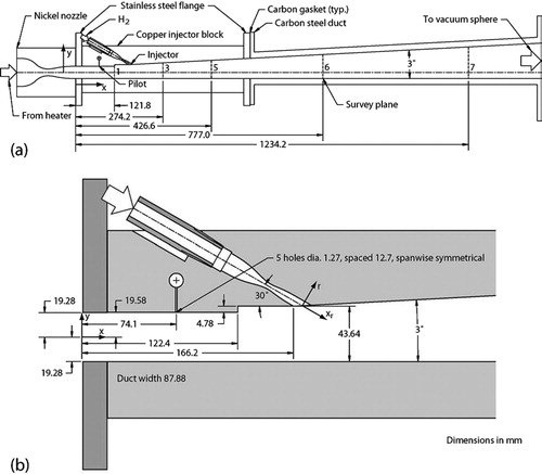
Figure 5. Grid topology of the SCHOLAR model.

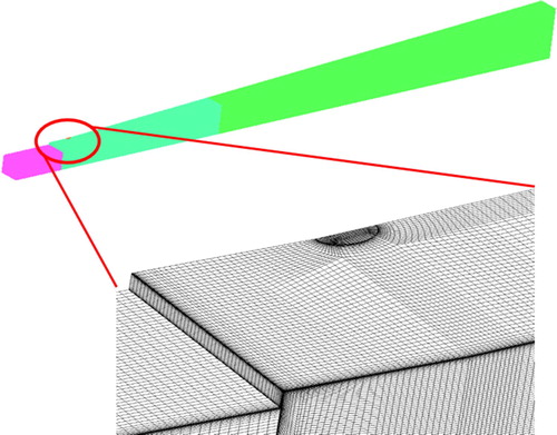
Table 2 shows the inlet boundary conditions for hydrogen and air. The inflow components include oxygen, nitrogen and water vapor with mass fractions of 0.2311, 0.5649 and 0.2040, respectively. Generally, inflow parameters such as the turbulence intensity have a great influence on simulation results (Rodriguez & Cutler, 2003, 2005). However, these values cannot be obtained by experiment but selected artificially from experience. In this study, 2% turbulent intensity and 200 turbulent viscosity ratio of air flow, 5% turbulent intensity and 10 turbulent viscosity ratio of hydrogen flow are assumed. In the experiment, the temperature of the copper wall in the isolator and the front part of the combustor varies from 350 to 500 K, while the latter part of carbon steel varies from 450 to 900 K. In the simulation, the wall is simplified as a non-slip boundary condition with a constant temperature of 475 K for copper and 700 K for carbon steel, which have been verified in the literature (O’Byrne et al., 2004) to show little influence on the simulation results of different wall temperatures.

Table 2. Inflow conditions of the SCHOLAR model.

	Hydrogen	Air
Ma	2.5	2.0
T (K)	133.0	1,204.0
P (Pa)	202,650.0	101,325.0
$Y_{\text{O}2}$	0.0	0.2311
$Y_{\text{N}2}$	0.0	0.5649
$Y_{\text{H}2\text{O}}$	0.0	0.2040
$Y_{\text{H}2}$	1.0	0.0

3.3. Numerical method

All the 3D RANS simulations are performed with CFDlab, a finite-volume code developed by CARDC. The inviscid fluxes are discretized using the Edwards Low Diffusion Flux Splitting Scheme (LDFSS) with the Van Leer flux limiter. The time iteration scheme acquires the Diagonalized Approximate Factorization (DAF). And the adaptive Courant-Friedrichs-Lewy (CFL) number is used for acceleration and stability. In order to investigate the interaction of turbulence and combustion through finite-rate chemistry models, a reduced but still accurate hydrogen kinetic mechanism with 9 species and 18 reactions from NASA Langley Research and Development Center is chosen (Rodriguez & Cutler, 2003). The Menter-SST model is used to close the Reynolds stresses and the turbulent dynamic viscosity.

4. Combustion results and discussion

4.1. DLR combustor

Since the interaction of turbulence and combustion is the most concerning part, the unburned flow-field analysis is neglected. The cases listed in Table 3 show the time consumption of each model in comparison with the case without the turbulent–chemistry interaction model (Case 1). Figure 6 presents the global structure and some differences between the shadow image captured in experiments (upper) (Oevermann, 2000) and the density contour of the simulation (lower). The global structure of the flow, which includes a widening reaction zone immediately after the strut and a constriction zone following on, is reproduced. In contrast to experiments, the combustion zone is narrower in the computed density contour and shifts downstream.

Figure 6. Shadow image of experiment (upper) and density contour of simulation (lower).

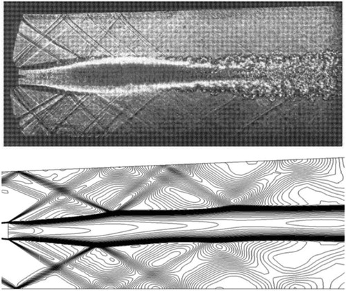
Table 3. Time required for the DLR model simulation cases.

Case	Turbulence–chemistry interaction model	Time consumption more than case 1 (%)
1	None	–
2	PaSR model	1.8
3	C-PaSR model	1.8
4	UPaSR model	28.6
5	C-UPaSR model	29.4

Since the distributions of the characteristic parameters simulated by the above models show little difference, the contours of the PaSR model are chosen as representative for analyzing the flow field. From the distribution of the characteristic parameters at the nozzle center in terms of its longitudinal section in Figure 7, it can be seen that ignition occurs in the reaction shear layer, which is formed by interaction of the hydrogen and air that come from the upper and lower edges of the wedge-shaped strut. Then a diffusion flame appears and stays stable in the wake region. In addition, two shock waves form at the leading edge of the strut and two expansion waves form at the rear edge reflecting from the wall of the combustor. All these structures form a complex wave system. As the pressure at the end of the strut increases after ignition, the shear layer no longer converges but expands to a height slightly wider than the strut. The supersonic reaction shear layer is relatively stable and thick. The reflected shock wave cannot penetrate. So reflection generates and the subsequent wave system between the wall and the shear layer forms. Meanwhile, the shear layer deflects and restricts the wake region expansion, which finally makes the flow in the wake region approximately parallel to the free stream. Therefore, the entire combustion area can be divided into three parts (Berglund & Fureby, 2007): an induction zone located from the bottom of the strut to the front of diffusion flame, where reaction occurs in the shear layer; a transition zone of large-scale coherent flow structures and convective mixing, where the concentration of OH radicals is high; and a turbulent combustion region. Contours of the Mach number and temperature are the most distinctive parameters to represent the above characteristics.

Figure 7. Characteristic contours of the PaSR model result in the center section.

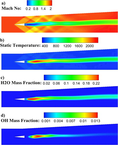
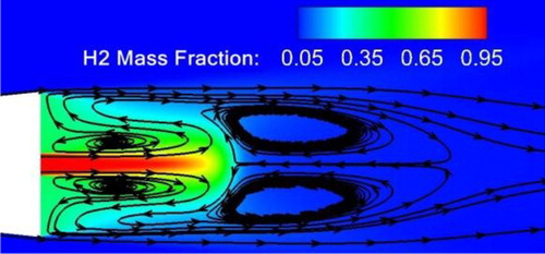
Turbulence–chemistry interaction models show little effect on fuel mixing in injection and recirculation regions. Streamlines around the nozzle in Figure 8 confirm that the flame locates at the reversed area of the induction zone. After the reversed area, the upper and lower shear layers converge into a central mixing layer, making the reaction concentrate near the center of the combustor. A large number of reaction intermediates and products assemble here. Therefore, the flame structure of such supersonic turbulent combustion behind a wedge-shaped strut is similar to a lifting flame. OH radical distribution is generally used to depict the flame structure. Figure 7(d) shows that it begins burning at 1–2 times the height of the strut after the wedge. Streamlines around the nozzle in Figure 8 confirm that the flame locates at the reversed area of the induction zone. After the reversed area, the upper and lower shear layers converge into a central mixing layer, making the reaction concentrate near the center of the combustor. A large number of reaction intermediates and products gather here. Therefore, the flame structure of such a supersonic turbulent combustion behind a wedge-shape strut is similar to a lifting flame.

Figure 8. Hydrogen field contour and streamlines in injection and recirculation regions.

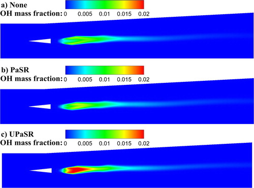
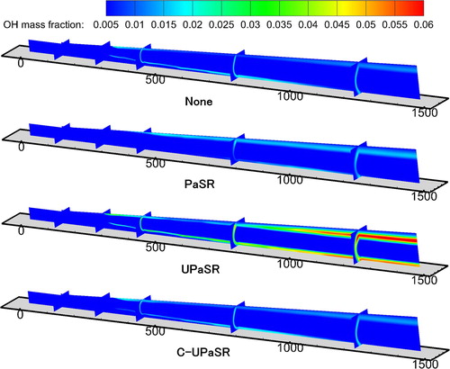
OH radical distribution is generally used to depict the flame structure. Figure 9 shows that all the cases begin burning at 1–2 times the height of the strut after the wedge. The flame concentrates in the transition zone and fades away gradually in the turbulent combustion zone. The PaSR model hardly changes the OH mass fraction distribution compared with the simulation without turbulence–chemistry interaction models. However, more OH radicals preserved in the center of the flame show that the UPaSR model obviously increases the quantity of reaction intermediates.

Figure 9. OH mass fraction contours of the case 1, 2 and 4 results in the center section.

The fine-scale structure volume fraction in the PaSR model and the UPaSR model ${\gamma }^{\ast }={\tau }_{ch}/({\tau }_{ch}+{\tau }_m)$ is the correction coefficient of the chemical reaction source term. It takes the turbulence time-scale and the chemical reaction time-scale to denote the relative intensity of the local mixing and combustion. Figure 10 shows that, except for the transition zone and the turbulent combustion zone, ${\gamma }^{\ast }=1$ in other regions, which means that combustion dominates the induction zone. This is in accordance with the analysis of the shear layer reaction above. The main difference between the PaSR model and the UPaSR model lies in the transition zone: ${\gamma }^{\ast }$ is relatively large in the PaSR model, close to 1.0 around the nozzle and smaller on the upper and lower sides, showing the same turbulent mixing and combustion effect. The UPaSR model has the smallest ${\gamma }^{\ast }$ and strongest inhibition effect in this region, which leads to significant influences on the parameter prediction in this region. The highest temperature and H₂O production are reduced, and the mass fractions of OH, O and H radicals are obviously increased. All phenomena present the UPaSR model suppress chemical reactions. The reasons may lie in the first simplification when solving the ordinary differential equations in Section 2.3. We are trying out the fully EPaSR model and will provide results in the future. After that, reaction in the stable combustion zone becomes weak, and any difference in ${\gamma }^{\ast }$ becomes inconspicuous.

Figure 10. Fine-structure volume fraction contours of the PaSR model and the UPaSR model.

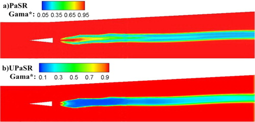
Figure 11 shows the temperature distribution at three different longitudinal sections. The experimental data and Oevermann’s simulation data are from Oevermann (2000). The results at X = 78 mm show that improvement is not obvious when the finite-rate chemistry model is used, and the bimodal curve of the temperature is not predicted. Menon and Fureby (Fureby et al., 2014; Génin & Menon, 2010) pointed out that this position is located in the wake region with high-intensity turbulence, which means accurate measurement in experiments is difficult. The result at X = 125 mm is satisfactory. The maximum temperature is revised by the PaSR model, but the horizontal scale of the mixing region is still slightly overestimated. The results of the C-UPaSR model show much more deviation. Combined with the result at X = 233 mm, the reason is that the maximum temperature prediction with the PaSR model is still slightly high. And the excessive temperature depression of the UPaSR model and C-UPaSR model mentioned above is clearly shown in this section. The temperature distribution at X = 233 mm is ideal after correction (Huang et al., 2015). Considering the turbulence–chemistry interaction, excessive maximum temperatures are suppressed, and the C-UPaSR model perfectly predicted the distribution in this region. As the temperature decreases away from the combustion area, the UPaSR model obtains an ideal result. In general, the finite-rate chemistry model is more reasonable for temperature prediction and can bring considerable correction with small costs. The result of the fine-scale structure reaction rate calculated by the UPaSR model equations is not improved, which needs future modification. It is speculated that the grid scale used in solving the volume fraction of the fine structure is the main influence. In LES, the grid scale is small, so the formula is accurate. But in RANS, it needs modification.

Figure 11. Static temperature distributions at different longitudinal sections.

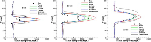
Figure 12 shows the axial velocity distribution at different sections. The upper left section describes results at Y = 25 mm, i.e. the axial velocity through the center of the nozzle. Compared with Figure 6, the reversed area is smaller, and the reverse velocity is higher in simulation cases than that in experiments. Four finite-rate chemistry models show little improvement in this respect.

Figure 12. Axial velocity distributions at different longitudinal sections.

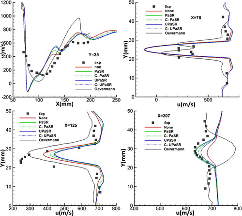
As for the other three sections, the axial velocity at X = 78 mm and X = 125 mm is not improved significantly. These two sections approximately locate at the beginning and the end of the transition zone, which means that at that position the interaction of turbulence and combustion is strongest. Although the result has been greatly modified after adopting finite-rate models here, it is still not satisfactory, which means that the correction is not enough to predict the bimodal structure of the axial velocity. Fureby (Fureby et al., 2014) obtained the bimodal characteristic at X = 78 mm under the condition of LES, and Oevermann (2000) achieved it by the flamelet model. It is speculated that, under the conditions of RANS, the flamelet model obtains better estimates than finite-rate chemistry models where mixing is intense. But the prediction of turbulence–chemistry interaction in LES is opposite, which is the field needing to be considered. And the reason for the velocity asymmetry in the experiment at X = 125 mm is still unknown. Many results of RANS and LES show the same phenomenon (Fureby et al., 2014; Huang et al., 2015; Oevermann, 2000). At X = 207 mm, the velocity difference between the wake region and the inflow decreases. The PaSR model and the UPaSR model reproduce the experimental data well. The C-PaSR model and the C-UPaSR model considering compressibility show slight deviation at the peak value. On the whole, finite-rate chemistry models can obtain ideal velocity results in the turbulent combustion region.

4.2. SCHOLAR combustor

There are a large number of factors affecting the SCHOLAR model simulation: grid scale, incoming flow turbulence intensity and viscosity ratio, wall temperature, incoming flow components and total temperature, dimensionless transport coefficients (the Prandtl and Schmidt numbers), the chemical reaction mechanism and so on. This study focuses mainly on the effects of the finite-rate chemistry model; hence, two grids (2.7 and 6.6 million) are selected to verify the grid independence, and case 2 is chosen as the benchmark case. All the cases are listed in Table 4.

Table 4. The SCHOLAR model simulation cases.

Case	Mesh number (millions)	Turbulence–chemistry interaction model
1	2.7	None
2	6.6	None
3	6.6	PaSR model
4	6.6	C-PaSR model
5	6.6	UPaSR model
6	6.6	C-UPaSR model

Rodriguez (Cutler et al., 2003; Rodriguez & Cutler, 2005) pointed out that the effect of mesh number is much less than other factors when a certain refined condition is constructed. Figure 13 illustrates a comparison of the pressure at the symmetric section of the upper and lower walls of the first two cases. It shows that a finer grid has little effect on pressure peak values. The pressure recovers from the shock reflection regions and shows nearly no difference at the outlet. Thus, this influence is neglected in further discussions.

Figure 13. Pressure distribution at the symmetric section of the upper wall (left) and the lower wall (right) for case 1 and case 2.

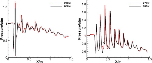
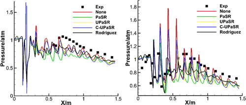
Figure 14 reveals the results of a comparison of the pressure along the axis of the upper and lower walls at the symmetrical section. Cocks et al. (2012), Keistler et al. (2007) and Rodriguez and Cutler (2003, 2005) simulated premixing and the reaction of hydrogen and air ahead of the inlet, showing that pressure oscillates in the isolator (Rodriguez line). In this study, simulations begin at the entrance of the isolation section, which do not show this phenomenon. However, this does not affect the combustion results (the first two peaks and valleys almost overlap). Before ignition, the benchmark case without turbulent–chemistry interaction models (the red lines) has higher pressure peaks, which means the combustion is more intense, and the ignition delay time is underestimated. The physical mixing time and reaction ignition time are two main aspects of these phenomena. The former is overestimated because of the turbulence model, and the latter is underestimated due to excessive chemical reaction speed. In the PaSR model case, the pressure peaks decrease significantly before ignition and the ignition delay time is corrected, which brings good agreement with the experimental data. The overall pressure alone the combustion wall decreases slightly after ignition, which is consistent with characteristics of the PaSR model. The UPaSR model recovers the entire pressure, but the peak value does not exceed the case without turbulent–chemistry interaction models, which indicates that the flow field is still dominated by suppression of the turbulence on combustion. Using the C-UPaSR model increases pressure slightly and promotes the combustion process. Overall, all the results reflect the tendency of the chemical reactions. Each finite-rate chemistry model shows little influence on the outlet pressure, but predictions of the pressure peaks and ignition delay time show accurate agreement with the experimental results.

Figure 14. Pressure distribution at the symmetric section of the upper wall (left) and the lower wall (right).

The ignition position and fuel penetration depth can easily be obtained from contours of the water mass fraction distribution at the symmetrical surface (Figure 15). When the turbulence–chemistry interaction model is not adopted, the ignition position is about 300 mm and starts simultaneously at the upper and lower walls.  The fuel penetration depth is up to about 600 mm. According to the pressure distribution in Figure 16, the ignition position on the upper wall is ahead of the intersection of the second reflected shock wave and upper wall. The high adverse pressure gradient and low velocity provide the environment for ignition. Introduction of the PaSR model significantly delays the ignition position and increases the fuel penetration depth to approximately 800 mm. The UPaSR model intensifies chemical reaction by modifying the fine-scale structure reaction rate, and restores it to the benchmark case. However, the C-UPaSR model shows that compressibility does not have significant impacts. In this example, it may be influence of the small turbulence intensity that leads to less obvious correction. Similar conclusions can be drawn from the pressure distribution contours.

Figure 15. Water mass fraction contours.

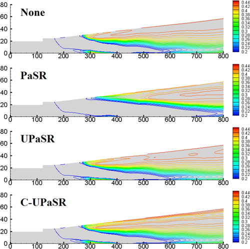
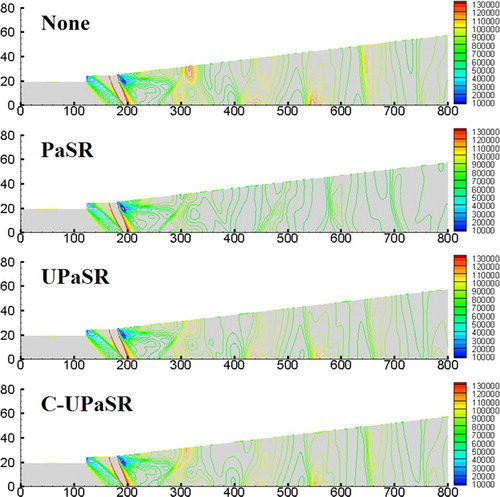
Figure 16. Pressure contours.

Flame structure revealed by contours of the OH mass fraction distribution (Figure 17) is in accordance with that in Figure 15. The PaSR model inhibits chemical reaction and hardly any flame structure can be seen at the bottom of the combustor. And the UPaSR model brings three times the OH mass fraction compared with the other cases. However, it hardly suppresses the highest temperature as the DLR model does. The reason is that the two turbulence–chemistry interaction models give similar fine-scale structure volume fractions ${\gamma }^{\ast }$.

Figure 17. OH mass fraction contours for different finite-rate chemistry models.

Further analysis of the chemical reaction region can be drawn from the temperature and oxygen mole fraction contours (Figures 18–20). In the experiments, seven slots were split for Coherent Anti-Stokes Raman Spectroscopy (CARS) measurement. They are numbered in Figure 4(a).

Figure 18. Temperature and oxygen mole fraction contours measured by CARS (experimental) and Rodriguez’s CFD results (numerical) (Rodriguez & Cutler, 2005).

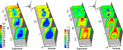
Figure 19. Temperature contours for different finite-rate chemistry models.

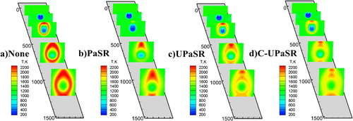
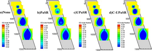
Figure 20. Oxygen mole fraction contours for different finite-rate chemistry models.

First of all, deviation of the temperature using the CARS method was ±70 K. The experimental measurement results were fitted by polynomial curves, which did not fully reflect the time-averaged results. In general, the range of the temperature in all simulations is consistent with the experiments, but the maximum temperature is slightly different in each condition. The results of the benchmark case without turbulence–chemistry interaction models are quite consistent with those in Rodriguez, which includes the temperature distribution, the range of the central low temperature zone and downstream of the reaction zone. The obvious disagreement is that, in all simulations, the reaction has already taken place at section 3, while the measurement result suggests that the reaction starts between sections 5 and 6. Only the case with the PaSR model shows a lower temperature and more oxygen in section 3, which agrees with the phenomenon in Figure 15. Generally, the temperature rises on the wall after the first reflection shock wave, which meets the requirement for reaction. Since the kinetic energy of the flow field is high, a slightly stronger shock wave predicted by simulation raises the pressure and temperature enough downstream of the decelerated fluid to react. In sections 6 and 7, the range of the low temperature zone in the center of the flame in all cases is larger than that in the experiments, which indicates that numerical simulations predict a longer fuel axial penetration depth. The turbulence model, which overestimates the mixing time-scale, needs to account for this phenomenon.

Comparing different finite-rate chemistry models, the PaSR model and the UPaSR model show better results. The former is more accurate in predicting the reaction region, but the high temperature zone at the lower wall surface in section 6 is not obtained because of the suppression effect. The penetration depth of the central low temperature zone deviates further from the experimental result. Although reaction has taken place in section 5 in the UPaSR model case, the high-temperature region decreases a lot compared to the case without turbulence–chemistry interaction models. Thereafter, the excessive temperature distribution is reduced in sections 6 and 7, and is not overly overestimated compared with experimental results like the PaSR model. However, temperature in the C-UPaSR model decreases more, which is opposite to the expected phenomenon. The reasons for this need further investigation.

Figure 20 shows the contours of the oxygen mole fraction. Compared with the CARS measurement distribution in Figure 18, all cases with turbulence–chemistry interaction models predict more accurate results. The PaSR model is the most desirable one. The concentration distributions predicted by the PaSR model in sections 3, 5 and 6 are in good agreement with the measurement results. Meanwhile, fuel injection near the nozzle and backflow from bottom to top in the central region can be observed, which reflects the actual flow field. On the other hand, a non-uniform oxygen distribution around the central area in the experiment is not observed for numerical cases, which may result from the non-uniform species distribution field at the outlet of the heater.

5. Conclusion

Based on typical turbulence–chemistry interaction models with finite-rate chemistry (the PaSR model and the UPaSR model), this study presents the C-PaSR model and C-UPaSR model to be suitable for numerical simulation of high Mach number chemical reaction flows by bringing in a compressibility correction. Results from two supersonic combustors have shown that the interaction between turbulence and combustion is intensive within complex supersonic chemical reaction flows. The time-scales of turbulence and chemistry are quite contrasting in different regions, which leads to the enhancement or weakening of the chemical reaction, and even self-ignition or extinction phenomena. It has been shown that, through validation against existing experimental data, taking the turbulence–chemistry interaction into consideration is necessary to capture the complex physical processes in supersonic turbulent combustion.

Detailed flow-field parameters manifest the effect of turbulence–chemistry interaction models and compressibility correction. The DLR model is a strut-inject combustor and its reaction flow field can be divided into three parts. The presented models show different modification effects due to the relative intensity between turbulence and chemical reaction in each region, which is revealed by the fine-scale structure volume fraction ${\gamma }^{\ast }$. The most evident improvement region begins downstream of the strut from a distance of approximately five times the strut length. The compressibility correction amends the temperature distribution and the effect of unsteady chemistry improves the velocity distribution. Moreover, computational time consumption is increased by the compressibility correction by less than 2%. For the SCHOLAR model with injection of hydrogen fuel from the top wall, the combustion area is larger and fuel jet penetration is deeper. The results show that the presented models modify the flow field, but it is difficult to obtain at the same time an improved wall pressure distribution, flow-field temperature distribution, fuel ignition delay distance and penetration depth. Each model has its own specific performance under different conditions. Other than the time-scales of mixing and chemical reaction, several aspects that influence the correction most (like local turbulence intensity) will also be the direction for the future. At present, the C-PaSR model and the UPaSR model present better results in all cases, which can be the choice for supersonic turbulent combustion with intense turbulence–chemistry interaction.

Disclosure statement

No potential conflict of interest was reported by the authors.

Additional information

Funding

The project is supported by the National Natural Science Foundation of China (No. 51706237 and No. 11902337).

References

- Akbarian, E., Najafi, B., Jafari, M., Ardabili, S. F., Shamshirband, S., & Chau, K.-w. (2018). Experimental and computational fluid dynamics-based numerical simulation of using natural gas in a dual-fueled diesel engine. Engineering Applications of Computational Fluid Mechanics, 12(1), 517–534. https://doi.org/10.1080/19942060.2018.1472670
- Baudoin, E., Yu, R., Bai, Nogenmyr, K. J., Bai, X. S., & Fureby, C. (2009). Comparison of LES models applied to a bluff body stabilized flame. Paper presented at the 47th AIAA Aerospace Sciences Meeting including The New Horizons Forum and Aerospace Exposition. January 5-8.
- Berglund, M., Fedina, E., Fureby, C., Tegner, J., & Sabel'nikov, V. (2010). Finite rate chemistry large-Eddy simulation of self-ignition in supersonic combustion Ramjet. AIAA Journal, 48(3), 540–550. https://doi.org/10.2514/1.43746
- Berglund, M., & Fureby, C. (2007). LES of supersonic combustion in a scramjet engine model. Proceedings of the Combustion Institute, 31(2), 2497–2504. https://doi.org/10.1016/j.proci.2006.07.074
- Bilger, R. W. (1993). Conditional moment closure for turbulent reacting flow. Physics of Fluids A: Fluid Dynamics, 5(2), 436–444. https://doi.org/10.1063/1.858867
- Charlette, F., Meneveau, C., & Veynante, D. (2002). A power-law flame wrinkling model for LES of premixed turbulent combustion part I: Non-dynamic formulation and initial tests. Combustion and Flame, 131(1–2), 159–180. https://doi.org/10.1016/S0010-2180(02)00400-5
- Cocks, P. A. T., Dawes, W. N., & Cant, R. S. (2011). The influence of turbulence-chemistry interaction Modelling for supersonic combustion. Paper presented at the 49th AIAA Aerospace Sciences Meeting including the New Horizons Forum and Aerospace Exposition. January 4-7.
- Cocks, P. A. T., Dawes, W. N., & Cant, R. S. (2012). Simulations of the SCHOLAR scramjet experiment. Paper presented at the 50th AIAA Aerospace Sciences Meeting including the New Horizons Forum and Aerospace Exposition. January 9-12.
- Cutler, A. D., Danehy, P. M., Springer, R. R., O’Byrne, S., Capriotti, D. P., & DeLoach, R. (2003). Coherent anti-stokes Raman spectroscopic thermometry in a supersonic combustor. AIAA Journal, 41(12), 2451–2459. https://doi.org/10.2514/2.6844
- Fureby, C., Fedina, E., & Tegnér, J. (2014). A computational study of supersonic combustion behind a wedge-shaped flameholder. Shock Waves, 24(1), 41–50. https://doi.org/10.1007/s00193-013-0459-2
- Génin, F., Chernyavsky, B., & Menon, S. (2003). Large Eddy simulation of scramjet combustion using a subgrid mixing/combustion model. Paper presented at the 12th AIAA internatoinal Space Planes and Hypersonic Systems and Technologies. December 15-19.
- Génin, F., & Menon, S. (2010). Simulation of turbulent mixing behind a strut injector in supersonic flow. AIAA Journal, 48(3), 526–539. https://doi.org/10.2514/1.43647
- Girimaji, S. S. (1991). A simple recipe for modeling reaction-rate in flows with turbulent-combustion. AIAA Journal. https://doi.org/10.2514/6.1991-1792
- Gonzalez-Juez, E. D., Kerstein, A. R., Ranjan, R., & Menon, S. (2017). Advances and challenges in modeling high-speed turbulent combustion in propulsion systems. Progress in Energy and Combustion Science, 60, 26–67. https://doi.org/10.1016/j.pecs.2016.12.003
- Huang, Z.-w., He, G.-q., Qin, F., & Wei, X.-g. (2015). Large eddy simulation of flame structure and combustion mode in a hydrogen fueled supersonic combustor. International Journal of Hydrogen Energy, 40(31), 9815–9824. https://doi.org/10.1016/j.ijhydene.2015.06.011
- Ingenito, A., & Bruno, C. (2008). Mixing and combustion in supersonic Reactive flows. Paper presented at the 44th AIAA/ASME/SAE/ASEE joint Propulsion Conference & Exhibit. July 21-23.
- Ingenito, A., & Bruno, C. (2009). Reaction regimes in supersonic combustion. Paper presented at the 47th AIAA Aerospace Sciences Meeting including The New Horizons Forum and Aerospace Exposition. January 5-8.
- Ingenito, A., & Bruno, C. (2010). Physics and regimes of supersonic combustion. AIAA Journal, 48(3), 515–525. https://doi.org/10.2514/1.43652
- Ingenito, A., Flora, M. G. D., Bruno, C., Giacomazzi, E., & Steelant, J. (2006a). Les modeling of scramjet combustion. Paper presented at the 44th AIAA Aerospace Sciences Meeting and Exhibit. January 9-12.
- Ingenito, A., Flora, M. G. D., Bruno, C., Giacomazzi, E., & Steelant, J. (2006b). A Novel model of turbulent supersonic combustion: Development and validation. Paper presented at the 42nd AIAA/ASME/SAE/ASEE joint Propulsion Conference & Exhibit. January 9-12.
- Karrholm, F. P. (2008). Numerical modelling of diesel spray injection, turbulence interaction and combustion (Doctoral dissertation). Chalmers University of Technology. https://www.mendeley.com/
- Keistler, P. G., Xiao, X., Hassan, H. A., & Cutler, A. D. (2007). Simulation of the SCHOLAR supersonic combustion experiments. Paper presented at the 45th AIAA Aerospace Sciences Meeting and Exhibit. January 8-11.
- Klimenko, A. Y. (1990). Multicomponent diffusion of various admixtures in turbulent flow. Fluid Dynamics, 25(3), 327–334. https://doi.org/10.1007/BF01049811
- Magnussen, B. F. (1981). On the structure of turbulence and a generalized eddy dissipation concept for chemical reaction in turbulent flow. Paper presented at the 19th AIAA Aerospace Science Meeting. January 12-15.
- Magnussen, B. F. (2005). The eddy dissipation concept: A bridge between science and technology. Paper presented at the ECCOMAS Thematic Conference on computational combustion, Lisbon, June 21-24.
- Magnussen, B. F., & Mjertager, G. H. (1976). On mathematical modeling of turbulent combustion with special emphasis on soot formation and combustion. Paper presented at the 16th Symposium (International) on combustion. December 1976. http://doi.org/10.1016/S0082-0784(77)80366-4
- Moule, Y., Sabelnikov, V., & Mura, A. (2014). Highly resolved numerical simulation of combustion in supersonic hydrogen–air coflowing jets. Combustion and Flame, 161(10), 2647–2668. https://doi.org/10.1016/j.combustflame.2014.04.011
- Moule, Y., Sabel'nikov, V., & Mura, A. (2011). Modelling of self-ignition processes in supersonic non premixed coflowing jets based on a PaSR approach. Paper presented at the 17th AIAA International Space Planes and Hypersonic Systems and Technologies Conference. April 11-14
- O’Byrne, S., Danehy, P. M., & Cutler, A. D. (2004). Dual-Pump CARS thermometry and species measurements in a supersonic combustor. Paper presented at the 42nd AIAA Aerospace Sciences Meeting and Exhibit. January 5-8.
- Oevermann, M. (2000). Numerical investigation of turbulent hydrogen combustion in a SCRAMJET using flamelet modeling. Aerospace Science and Technology, 4(7), 463–480. https://doi.org/10.1016/S1270-9638(00)01070-1
- Petrova, N. (2015). Turbulence-chemistry interaction models for numerical simulation of aeronautical propulsion systems. The Ecole Polytechnique.
- Rodriguez, C. G., & Cutler, A. D. (2003). CFD analysis of the SCHOLAR scramjet model. Paper presented at the 12th AIAA International Space Planes and Hypersonic Systems and Technologies. December 15-19.
- Rodriguez, C. G., & Cutler, A. D. (2005). Computational simulation of a supersonic-combustion benchmark experiment. Paper presented at the 41st AIAA/ASME/SAE/ASEE joint Propulsion Conference & Exhibit. July 10-13.
- Sabelnikov, V., & Fureby, C. (2011). Extended LES-PaSR model for simulation of turbulent combustion. Paper presented at the 4th EUROPEAN CONFERENCE FOR AEROSPACE SCIENCES (EUCASS). July 4-8.
- Sabelnikov, V., & Fureby, C. (2012). LES combustion modeling for high re flames using a multi-phase analogy. Combustion and Flame. https://doi.org/10.1016/j.combustflame.2012.09.008
- Sabelnikov, V., & Fureby, C. (2013). Extended LES-PaSR model for simulation of turbulent combustion. Progress in Propulsion Physics, 4, 539–568. https://doi.org/10.1051/eucass/201304539
- Safer, K., Bounif, A., Safer, M., & Gökalp, I. (2010). Free turbulent reacting jet simulation based on combination of transport equations and PDF. Engineering Applications of Computational Fluid Mechanics, 4(2), 246–259. https://doi.org/10.1080/19942060.2010.11015314
- Saghafian, A., Shunn, L., Philips, D. A., & Ham, F. (2014). Large eddy simulations of the HIFiRE scramjet using a compressible flamelet/progress variable approach. Proceedings of the Combustion Institute. https://doi.org/10.1016/j.proci.2014.10.004.
- Saghafian, A., Terrapon, V. E., & Pitsch, H. (2015). An efficient flamelet-based combustion model for compressible flows. Combustion and Flame, 162(3), 652–667. https://doi.org/10.1016/j.combustflame.2014.08.007
- Turns, S. R. (2012). An introduction to combustion: Concepts and applications (3rd ed.).
- Williams, F. A. (2000). Progress in knowledge of flamelet structure and extinction. Progress in Energy and Combustion Science, 26(4–6), 657–682. https://doi.org/10.1016/S0360-1285(00)00012-5
- Wirth, M., & Peters, N. (1992). Turbulent premixed combustion: A flamelet formulation and spectral analysis in theory and IC-engine experiments. Paper presented at the Twenty-Fourth Symposium (International) on combustion. July 5-10.
- Zhao, G.-Y., Sun, M.-B., Wu, J.-S., & Wang, H.-B. (2015). A flamelet model for supersonic non-premixed combustion with pressure variation. Modern Physics Letters B, 29(21), 1550117. https://doi.org/10.1142/S0217984915501171