Design optimization of a vane type pre-swirl nozzle

Abstract

Pre-swirl system is installed to minimize energy loss between the stationary and rotating parts of turbine secondary air system. Although various optimization studies were conducted to increase the pre-swirl efficiency, most of the studies were focused on a hole type pre-swirl nozzles. In this study, a vane type pre-swirl nozzle was optimized to increase mass flow rate and temperature drop for given boundary conditions. The system performance was analyzed by 3D CFD and the objective functions were used to maximize the discharge coefficient and the adiabatic effectiveness. After sensitivity analysis, seven design variables were chosen on the three planes of nozzle span-wise direction. The OLHD method was used to obtain the initial scattered test points, and the additional ones were supplied by the ALHD method. The Kriging model was constructed as the surrogate one, and refined iteratively until satisfying the convergence criteria between the estimated point and the CFD result. The optimized model improved the span-wise uniformity of the flow path and the discharge coefficient was increased by 2.57%, whilst the adiabatic effectiveness remained nearly constant. The performance was also analyzed for pressure ratio and off-design points, with the optimized model showing better performance at all boundary conditions.

KEYWORDS:

• Adiabatic effectiveness
• discharge coefficient
• MOGA
• pre-swirl system
• secondary air system
• vane type nozzle

Nomenclature

A	=	Pre-swirl nozzle throat area (m2)
b	=	Outer radius at the cavity (m)
c	=	Velocity in absolute frame of reference (m/s)
CD	=	Discharge coefficient of the pre-swirl system
CDN	=	Discharge coefficient of the pre-swirl nozzle
CW	=	Non-dimensional mass flow rate (= $\dot{m}$/$\mu b$)
Cp	=	Static pressure coefficient
cp	=	Specific heat at constant pressure (J/ kg·K)
k	=	Turbulence kinetic energy (m2/s2)
$\dot{m}$	=	Mass flow rate (kg/s)
r	=	Radius (m)
P	=	Pressure (N/m2)
ReØ	=	Rotational Reynolds number (= Ω·b2/${\nu }_1$)
T	=	Temperature (K)
vØ	=	Circumferential velocity (m/s)
w	=	Velocity in relative frame of reference (m/s)
y+	=	Non-dimensional wall distance

Greek

β	=	Swirl ratio (= vø/ Ω·r)
γ	=	Specific heat ratio
λT	=	Turbulent flow parameter (= CW·Reø−0.8)
µ	=	Coefficient of viscosity (N·s/${\text{m}}^2$)
$\nu$	=	Kinematic viscosity (m2/s)
ω	=	Turbulence eddy frequency (s−1)
$\mathrm{\Theta }$	=	Adiabatic effectiveness
Ω	=	Angular velocity of rotor (rad/s)

Subscript

0	=	Pre-swirl nozzle inlet
1	=	Pre-swirl nozzle outlet
2	=	Receiver hole inlet
3	=	Receiver hole outlet
rel	=	Relative frame of reference
s	=	Static
t	=	Total

1. Introduction

The recent trend in modern gas turbine operation involves increasing compressor pressure ratio and TIT (Turbine Inlet Temperature) to improve turbine efficiency and the generated power. Currently commercial H class industrial gas turbines have a TIT up to 1650°C. For such a system to operate reliably, it is necessary to improve the secondary cooling flow path design for efficient cooling of the turbine components.

To this end, within the operating conditions specified to meet the target performance, the secondary air system should be designed primarily for supplying cooling air with appropriate pressure, temperature, and mass flow rate to each row of the turbine blades. In this case, a pre-swirl system is installed for reducing energy loss of the cooling air moving from the stationary to rotating parts. By inducing a flow angle in advance, the pressure loss can be minimized to maintain both pressure and mass flow rate as high as possible in the rotating cooling path. In addition, because of the relatively high circumferential velocity of the cooling air, the relative total temperature at the rotating parts is decreased. Hence, a well-designed pre-swirl system can help reducing the amount of cooling flow, and ultimately, can improve turbine performance.

Efficiency of the pre-swirl system is analyzed by temperature drop and mass flow rate. Wilson et al. (1997) conducted both experimental and numerical study on a direct-transfer pre-swirl system in which the pre-swirl nozzles and the receiver holes were mounted at the same radial location. By measuring the flow field and temperature distribution in the receiver hole, it was confirmed that the temperature drop of the cooling air was increased as the swirl ratio was increased. Ditmann et al. (2002) experimentally investigated the relationship between the geometries of receiver holes and flow energy loss in a direct-transfer pre-swirl system. Experimental data were compared with CFD (Computational Fluid Dynamics) results for various receiver hole geometries, as well as the pressure ratio. In addition, the discharge coefficient of the pre-swirl system, which is the ratio between the actual mass flow rate and the ideal one, was defined at each measurement point based on a theoretical formula and a loss factor due to friction or mixing. The discharge coefficient of the hole type pre-swirl nozzle was affected by the number of receiver holes and the circumferential velocity component of the fluid. The pre-swirl system discharge coefficient was between 0.7 and 0.8.

Since the location and design method of the pre-swirl system used to achieve the design requirements for each gas turbine model are different, extensive research has been performed to optimize the design parameters and to incorporate them into gas turbines. There are typically four components of a pre-swirl system: inlet duct, pre-swirl nozzle, cavity and receiver hole. Numerous studies on each component have been carried out. For the inlet duct, the effect of the internal support structure and shape optimization were studied to improve performance (Kim et al., 2018; Lee et al., 2018). Compared with the original model, the new design for the internal structure and pre-swirl nozzle showed improvement in the discharge coefficient and adiabatic effectiveness. On the other hand, the direct-transfer pre-swirl system showed a small change in system efficiency with cavity shape (Bricaud et al., 2007; Ditmann et al., 2002). Studies on the shape of the receiver hole have also been carried out (Bricaud et al., 2007; Didenko et al., 2012; Ditmann et al., 2002). The ratio of the nozzle throat area to the receiver hole inlet area was the most influential shape parameters, and system efficiency was highest for the full annulus outlet without receiver holes.

Among the components of the pre-swirl system, research on the pre-swirl nozzle has been the most prevalent. Depending on nozzle shape, it can be classified into a hole or vane type, and the vane type nozzle shows a relatively higher performance. In early work, CFD validations for hole type nozzles were widely conducted because of their simple geometries. However, recently, a variety of performance improvement studies have been conducted on the shape of the vane type nozzle. Kim et al. (2018) studied various shapes of aerofoil for pre-swirl nozzles. A basic vane type nozzle which generally has better performance than a hole type nozzle, was designed. The performance curves of pre-swirl system with different number of nozzles, i.e. different throat areas, for various boundary conditions were also provided in the study.

Several creative designs have been applied to the vane type nozzle in many studies. Javiya et al. (2011) investigated three types of pre-swirl nozzles: the simple hole type, the aerodynamically designed hole type, and the vane type. The discharge coefficient and temperature drop were compared, with the vane type nozzle showing the best performance in both parameters. Liu et al. (2016) proposed a new concept VSH (Vane Shaped Hole) nozzle with increased solid width and sharp trailing edge compared to the general cascade vane type nozzle and compared its performance to that of conventional models. Lee et al. (2018) arranged VSH nozzles at regular intervals between general cascade vane type nozzles to minimize energy loss from the internal support structure at the inlet duct. Kim et al. (2017) suggested a new pre-swirl nozzle configuration with a splitter. The authors showed that the aerodynamic loss and swirl ratio could be increased by adjusting the position of a splitter installed between the cascade vane type nozzles.

For both hole type and vane type nozzles, shape optimization has been studied to improve pre-swirl performance. Ciampoli et al. (2007) performed shape optimization for the outlet diameter and the flow path of hole type pre-swirl nozzles. The SA (Simulated Annealing) algorithm was used as an optimization method and the results were compared with those of the DHC (Dynamic Hill Climbing) algorithm and the RSM (Response Surface Model) methodology. It was found that the optimal solution using RSM showed a higher discharge coefficient, which was 0.83 without considering the rotating effect. Lee et al. (2019) optimized the hole type nozzle using the OLHD (Optimal Latin Hypercube Design) method and a genetic algorithm. It was shown that the discharge coefficient of the optimal model was 31.7% higher than that of the initial model by optimizing the angle of convergence and reducing the blockage effect.

To improve the efficiency through various shape parameters, many studies have been conducted on the validation of CFD methodology and experimental results (Park et al., 2019; Ramezanizadeh et al., 2019). However, most of the gas turbine pre-swirl nozzle studies were concentrated on the hole type pre-swirl system. In this study, 3D optimization of a vane type nozzle was conducted to compare the results in terms of discharge coefficient and adiabatic effectiveness. In addition, the pre-swirl performance change under off-design conditions was analyzed.

2. Theoretical approach

2.1. Discharge coefficient (C_D)

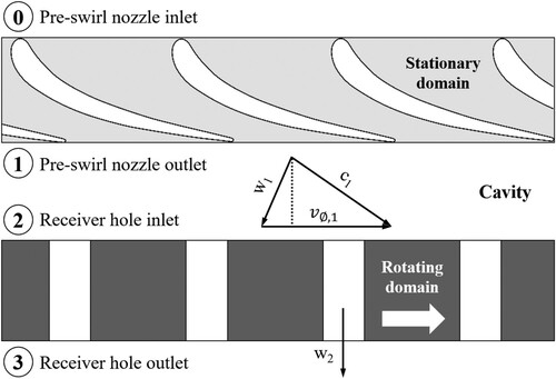
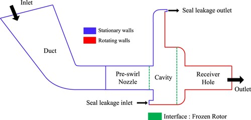
The discharge coefficient is a non-dimensional indicator of the performance of the pre-swirl system applied by Ditmann et al. (2002). It represents the ratio of the mass flow rate to the theoretical one. The discharge coefficient goes to 1 as the pre-swirl system efficiency increases. High pre-swirl efficiency also means that the cooling mass flow rate supplied to the nozzle throat area increases. The discharge coefficient were defined for the number of measurement locations shown in Figure 1.

Figure 1. Schematic view of the pre-swirl system.

Equation (1) describes the discharge coefficient at the nozzle outlet (C_DN), whilst Equation (2) shows the discharge coefficient of the entire pre-swirl system (C_D). (1) $\begin{array}{rl}{C}_{DN}& =\frac{{\dot{m}}_1}{\frac{A{P}_{0t}}{\sqrt{R{T}_{0t}}}\sqrt{\frac{2\gamma }{\gamma -1}\left[{\left(\frac{P_{1s}}{P_{0t}}\right)}^{\frac{2}{\gamma }}-{\left(\frac{P_{1s}}{P_{0t}}\right)}^{\frac{\gamma +1}{\gamma }}\right]}}\end{array}$(1) (2) $\begin{array}{rl}{C}_D& =\frac{{\dot{m}}_3}{\frac{A{P}_{0t}}{\sqrt{R{T}_{0t}}}\sqrt{\frac{2\gamma }{\gamma -1}\left[{\left(\frac{P_{3s}}{P_{0t}}\right)}^{\frac{2}{\gamma }}-{\left(\frac{P_{3s}}{P_{0t}}\right)}^{\frac{\gamma +1}{\gamma }}\right]}}\end{array}$(2) For comparing mass flow rates for various turbines sizes, non-dimensional mass flow rate C_W was introduced in Equation (3). The mass flow rate at 1 and 3 (as shown in Figure 1) could be slightly different due to cavity seal leakage. (3) $C_{1W}=\frac{{\dot{m}}_1}{{\mu }_{1}b}\text{or}{C}_{3W}=\frac{{\dot{m}}_3}{{\mu }_{3}b}$(3) As the discharge coefficient represents the flow efficiency at a particular nozzle throat area, mass flow rate could decrease even though the discharge coefficient increases, if throat area is decreased. Hence, the mass flow rate as well as the discharge coefficient should be considered for analyzing the performance of an actual system.

2.2. Adiabatic effectiveness (θ)

The temperature drop performance of a pre-swirl system was evaluated using adiabatic effectiveness θ (Karabay et al., 1999), which is shown in Equation (4). This non-dimensional number is derived from the equation between work to air and kinetic energy, which represents the ratio of enthalpy change to rotational kinetic energy. (4) $\theta =\frac{c_p|T_{2t,rel}-T_{1t}|}{\frac{1}{2}{r}^2{\mathrm{\Omega }}^2}$(4) Adiabatic effectiveness means that the pre-swirl system is efficiently achieving the total temperature drop in the rotating coordinate system, and adiabatic effectiveness and swirl ratio have a linear relationship in all the sections. When the adiabatic effectiveness becomes 1, the swirl ratio also becomes 1. Note that the swirl ratio β shown in Equation (5) is defined as the ratio of the circumferential velocity of the flow at the outlet of the pre-swirl nozzle to rotational speed of the turbine disk at the same radius. (5) $\text{β}=\frac{v_{\text{o}}}{\mathrm{\Omega }r}$(5) Rotational speed of the turbine disk and the circumferential velocity of the flow at the outlet of the pre-swirl nozzle coincide when the swirl ratio is 1, which is the best operating condition for minimizing pressure drop, whilst ensuring minimum relative total temperature.

3. CFD methodology

3.1. Numerical analysis and validation

In this study, to analyze the behavior of fluids under steady state conditions, the solution of the RANS (Reynolds-Averaged Navier-Stokes) equation was obtained using a CFD tool ANSYS CFX 2019 R3. The SST (Shear-Stress Transport) k-ω turbulence model was applied as the turbulence model (Javiya et al., 2012), which is suitable when the numerical analysis of the flow inside a rotating region is complicated and the viscous region of the wall must be considered.

The initial code validation of this study was conducted based on the data reported from open literature contributions. The experiment data conducted at University of Bath, UK were compared with CFD results, along with applying the same boundary conditions. The sketch of the test rig and computational domain are shown in the Figure 2.

Figure 2. Test rig and computational domain (Javiya et al., 2012).

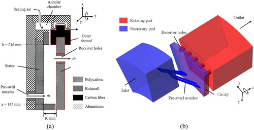
The cover-plate pre-swirl system experiment was conducted with an inner radius a = 145 mm and outer radius b = 216 mm. The pre-swirl nozzles were composed of 24 holes, and 20° inclined to the circumferential direction. The radial location of the nozzles was r = 160 mm and its diameter was 7.1 mm. 60 receiver holes were located at r = 200 mm with a length-to-diameter ratio of 1.25. For more details, Bath experimental setup can be found in Javiya et al. (2012). Referring to the recently studies, the computational domain was extended tangentially 30° including two pre-swirl nozzles and five receiver holes instead of annular slots. Periodic condition was applied at each tangential side and frozen rotor interface was applied between the stationary and rotating domains.

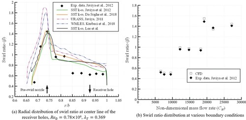
The radial distribution of the swirl ratio for fixed boundary conditions and the swirl ratio according to various boundary conditions were shown in Figure 3 (Da soghe et al., 2018; Kusbeci & Chew, 2018). In Figure 3(a), the experimental data and the CFD result showed a tendency to fit quite well, and the largest discrepancy (26%) was captured around r/b = 0.85. This area was similarly calculated in previous studies and was considered to be due to the weakness of the RANS turbulence model which generally underestimates jets spreading and mixing. On the other hand, in the case of Figure 3(b), which compared the averaged swirl ratio on the interface, showed very similar results for each boundary conditions, and the average error was 3.69%.

Figure 3. Comparative analysis of swirl ratio.

Based on the above results, Hanyang University conducted an experiment on the direct-transfer pre-swirl system to verify the discharge coefficient, and compared it with the CFD results. The test rig used in the experiment is shown in Figure 4.

Figure 4. Hanyang University direct-transfer pre-swirl system test rig.

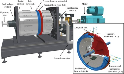
Test rig was designed 1/2 of the actual machine size using the similarity law, and 60 vane type pre-swirl nozzles and 68 receiver holes were installed. Fixed sensors which measured pressure and temperature were equipped at pre-swirl nozzle inlet, pre-swirl nozzle outlet, and receiver hole outlet. Total mass flow rate and seal leakage could be checked by measuring the mass flow rate at inlet and outlet of the system. Radial span of pre-swirl nozzle was 30 mm and the parameter range tested in the experiment was 0.6 < ${\lambda }_T$<1.34, $0.4\times {10}^6<{\text{Re}}_{\varphi }<1.5\times {10}^6$, and $0.67<\text{β}<1.82$. In this test rig, experiments were conducted for each nozzle model and boundary conditions, and the results are shown in Figure 5.

Figure 5. Result of experiment and CFD (a) Lee et al. (2020), (b) Lee et al. (2019).

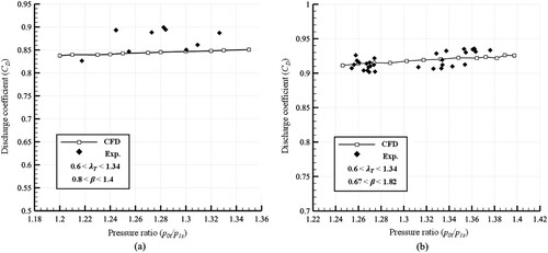
As a result of comparative analysis of the experimental data and numerical analysis, overall reasonable results were obtained. In both graph, the discharge coefficient increased as the pressure ratio increase due to the compressibility effect.

3.2. Geometrical configurations

The base vane type pre-swirl nozzle, designed based on NACA0010, has constant cross-section. The secondary air system was designed as a direct-transfer pre-swirl system in which 60 pre-swirl nozzles and 68 receiver holes were located at the same radius from the center of rotation. To derive the design parameters of the vane type pre-swirl nozzle, seven independent shape parameters were defined for each of three cross-sectional planes in a span-wise direction, as shown in Figure 6.

Figure 6. Vane design parameters.

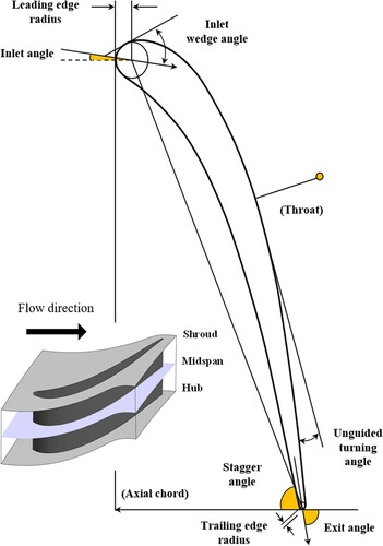
The defined shape parameters were inlet angle, leading edge radius, stagger angle, exit angle, unguided turning angle, and trailing edge radius. Among eleven of the shape parameters considered by Pritchard (1985) for gas turbine vane shape, the design variables were defined by excluding the uncontrollable variables, including the constraints and dependent variables given in the overall system. In addition, the stagger angle was added as a shape parameter to provide a high circumferential velocity component at the nozzle outlet.

Computational analysis was performed to analyze the discharge coefficient of the vane type pre-swirl nozzle as shown in Figure 7. Only one axisymmetric 3D flow path was calculated, by applying the periodic condition to decrease the calculation time. The fluid domain consisted of a stationary part (a pre-swirl nozzle) and a rotating one (a receiver hole).

Figure 7. Computational domain of the pre-swirl system.

3.3. Grid independency

As shown in Figure 8, the girds used around the vane type pre-swirl nozzle were generated as block-structured hexagonal grids using ANSYS TurboGrid, and other analysis domains consisted of tetrahedral and prism grids. In the nozzle region where the shape was modified for optimization, the same number of hexahedral grids were re-meshed by the batch files even if the design variables had been changed. A sufficient number of hexagonal layers were generated in order to resolve the boundary layer on the near-wall of the analysis region accurately. The maximum y⁺ was less than 1 at the all domain through inflation layers.

Figure 8. Computational grids for numerical analysis.

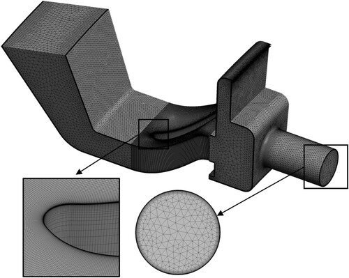
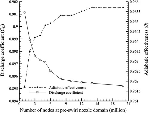
Figure 9 shows the grid independency test to determine the number of grids for the fluid domain, where the error was less than 0.1% for 6 million or more grids. As a result, 8.2 million grids were generated in total: 6 million in the pre-swirl nozzle domain and 2.2 million in the remaining ones. Based on the RMS (Root Mean Square) values, the solution convergence for all residuals was satisfied at less than $1\times {10}^{-4}$. Also, for all domains, mass flow rate and angular momentum imbalance were less than $4\times {10}^{-5}$.

Figure 9. Grid independency test.

3.4. Boundary conditions

Calibrated ideal gas was applied as the working fluid, which properties were corrected using the characteristics of ideal gas (Kim et al., 2016). The entire system was modeled with four separate domains, with the GGI (General Grid Interface) and the frozen rotor methods being used for the interface between the stationary and rotating parts (Benim et al., 2004). Since the pre-swirl system shows an irregular flow field at the nozzle outlet and a large velocity distribution in the circumferential direction, the frozen rotor interface is suitable for analysis of the pre-swirl system. To create a periodic annulus interface to calculate the rotating receiver hole domain, one axial plane in the cavity domain was selected as the frozen rotor interface. The walls in the cavity adjacent to the rotating domain were treated as rotating walls to simulate the rotating disk. Dependency of the inlet turbulence quantities was checked, and the difference between each results was insignificant. Therefore, the turbulence intensity was assumed to be 5%.

Boundary conditions were applied in consideration of the fluid properties given to SAS (Secondary Air System) from the total system design. The inlet conditions at the entrance of the pre-swirl system were 20 bar of total pressure and 700 K of total temperature which were discharged from the compressor. The outlet condition was 16.53 bar of static pressure, and the disk rotating speed was 3600 rpm. Except for the periodic ones, the walls were set to no-slip and were adiabatic. The summarized boundary conditions are shown in Table 1.

Table 1. Boundary conditions of the pre-swirl system.

Inlet		Outlet
Total pressure	Total temperature	Static pressure
20 bar	700 K	16.53 bar
Seal leakage in		Seal leakage out
0.006 kg/s		0.003 kg/s

4. Optimization

4.1. Defining optimization problems

In order to conduct the optimization process efficiently, the nozzle throat area change was limited to ± 1% of the initial design value. In this study, since the constant static pressure ($p_{3s}$) boundary condition was applied to the receiver hole outlet, the objective function could be re-defined as a relation of the mass flow rate ($\dot{m})$, static pressure ($p_{1s}$) and total temperature (T_1t). Given a constant rotating speed and receiver hole outlet pressure with fixed throat area of pre-swirl nozzle, the discharge coefficient at the outlet of pre-swirl nozzle (C_DN) and that of the entire pre-swirl system (C_D) have a linear relationship. Hence, in this study, the discharge coefficient and adiabatic effectiveness at the pre-swirl system outlet were used as the objective functions.

Objective.

Max. System discharge coefficient (C_D$)$

Max. System adiabatic effectiveness ($\theta$)

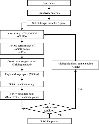
Constraint. $|A_{initial}-A|\le 0.01\times A_{initial}$A commercial optimization tool PIAnO was used for the design of experiment, surrogate model construction, and optimization, the lattermost process being shown in Figure 10.

Figure 10. Flow chart of the optimization process.

4.2. Sensitivity analysis of design variables

As shown in Figure 11, sensitivity analysis of each variable was performed by defining the upper and lower limits of the shape parameters. The stagger and exit angles, having large effects on the shape of the flow path, were limited to ± 3% of the initial value and the remaining design variables were constrained to ± 5% of this value. The results of the sensitivity analysis for each design variable are shown in Figure 7, where the variation of the discharge coefficient and adiabatic effectiveness for each design variable are shown. The stagger and exit angles had the biggest effects on the discharge coefficient and the adiabatic effectiveness. In addition, to confirm the optimization tendency of the design variables with non-significant sensitivity, the hub unguided turning angle was selected as an additional parameter. It showed a relatively high sensitivity among the less sensitive design variables. The design boundary was defined within the range of 4% except unguided turning angle in the hub. The final design parameters and non-dimensional design boundaries are shown in Table 2.

Figure 11. Sensitivity analysis of the discharge coefficient and the adiabatic effectiveness.

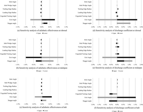
Table 2. Selected design variables and normalized design space.

Design variables		Lower bound	Initial value	Upper bound
Shroud	Stagger angle	0.969	1	1.031
	Exit angle	0.963	1	1.038
Midspan	Stagger angle	0.969	1	1.031
	Exit angle	0.963	1	1.038
Hub	Stagger angle	0.969	1	1.031
	Exit angle	0.963	1	1.038
	Unguided turning angle	0.667	1	1.333

4.3. Design of experiment

As the design optimization is computationally expensive, it is essential to select appropriate test points for minimizing the resources required in this respect. In this study, the OLHD (Optimal Latin Hypercube Design) method was used to obtain the test points efficiently and 54 initial test points were selected for seven design variables (Lee et al., 2013). The OLHD method maximizes the variance of the test points and improves the bias of the test points, thus overcoming a disadvantage of the LHD (Latin Hypercube Design) method. That is, an efficient approximation model with fewer test points can be constructed with the OLHD method. In addition, to improve the reliability of the approximation model constructed with the OLHD method, 10 additional test points were added incrementally using the ALHD (Augmented Latin Hypercube Design) method. In order to complement the initial test points, the ALHD method was used to improve the space-filling function for the test points. In this manner, a reliable response surface can be generated for the interaction of the variables (Montgomery et al., 2009; Myers et al., 2004).

4.4. Surrogate model

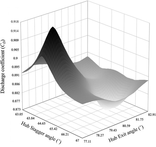
A surrogate model was constructed based on the computational analysis results of the selected test points, and the Kriging model was used as this model. The Kriging model is composed of the global model and the localized deviation as one of the interpolation methods. It is suitable for numerical calculation because of its high reliability of approximation for a second-order (or higher) non-linear system (Ahmed & Qin, 2009). The response surface of the stagger and exit angles with respect to the discharge coefficient are shown in Figure 12.

Figure 12. Kriging model of hub stagger angle and hub exit angle with respect to the discharge coefficient.

4.5. Optimal point

The MOGA (Multi-Objective Genetic Algorithm) was used to derive the optimum point based on the surrogate model. Like the GA (Genetic Algorithm), MOGA uses the mathematical algorithms of natural genetic evolution, but whilst simultaneously optimizing one or more objective functions. In this algorithm, various solutions can be determined according to the selection criteria of the optimum solution to find a representative set of Pareto optimal solutions. The goal of this optimization process is to ensure the quantity of trade-offs within a range that can satisfy each objective function, and to find a single solution that meets the subjective preferences of the decision maker (Fonseca & Fleming, 1993).

According to the MOGA result, as shown in Figure 13, the Pareto optimal solution graph was derived and a single optimal solution was chosen by the decision maker. A higher weighting factor was given to the discharge coefficient because the system performance was far less sensitive to the adiabatic effectiveness than the discharge coefficient.

Figure 13. Pareto optimal solution graph.

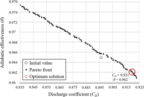
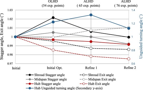
Figure 14 shows the pre-swirl system discharge coefficient between the candidate point of the Kriging surrogate model and the calculated CFD result. Two refinement steps were conducted and 10 test points were added at each step to find the global optimal point. The optimization process was terminated when the error between the two values was less than 0.5%. When the refinement was repeated, both the candidate point and the CFD result increased whilst the error between the two decreased. After applying the ALHD method to improve the surrogate model, the changes of optimal design values of each variable for the initial optimization (OLHD) and the refined ones (ALHD) were obtained, as shown in Figure 15.

Figure 14. Comparison of the candidate point of Kriging model and CFD result.

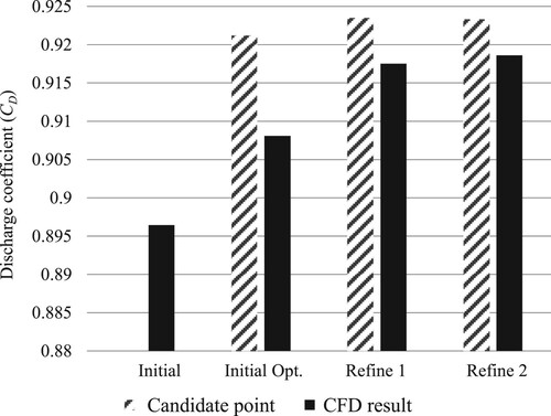
Figure 15. Normalized optimum points in design space in accordance with the refinement steps.

5. Result

5.1. Optimization

The derived optimal design values of each variable are shown in Table 3, where non-dimensional numbers are used to show relative dimensions compared to each dimension of the initial model. The optimized and initial models are simultaneously shown in Figure 16.

Figure 16. Comparison of the initial and optimized models.

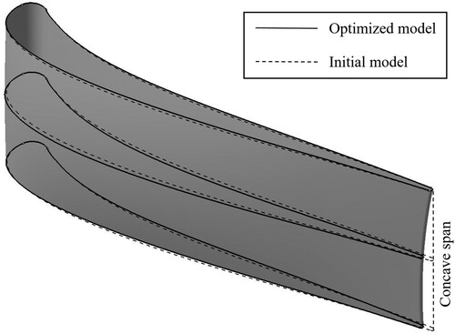
Table 3. Normalized optimal design variables.

Shroud stagger angle	0.999	Hub stagger angle	0.991
Shroud exit angle	0.986	Hub exit angle	0.975
Midspan stagger angle	0.992	Hub unguided turning angle	1.127
Midspan exit angle	1.01

The optimized discharge coefficient (C_D) and adiabatic effectiveness (θ), for the given properties at the pre-swirl system outlet, are shown in Table 4, along with the dimensionless mass flow rate (C_W) and swirl ratio (β).

Table 4. Optimization results.

	Initial model	Opt. model	Δ (%)
CD	0.896	0.919	2.57
CW	31867	32752	2.78
θ	0.965	0.961	−0.41
β	1.009	1.006	−0.3

As a result of optimization, the system exit discharge coefficient increased by 2.57% compared with the initial model. The difference in the nozzle throat area between the optimized and initial model was kept within 0.1%. Whilst the adiabatic effectiveness decreased by 0.41%, the swirl ratio remained higher than 1 and the relative total temperature at the system outlet increased only by 0.13 K. This is due to the high weighting factor applied to the discharge coefficient, which implies improved pre-swirl system performance.

Compare with the initial model, in the hub and the shroud, the vane cross-section was optimized to have a smaller camber. On the other hand, in the midspan section, the optimized vane had a larger one. Also, as the chord length of the optimized vane was shorter in the hub and midspan than the shroud, the trailing edge of the vane had a concave shape in the span-wise direction (Figure 16). Unlike the hub and the shroud, there is no extra wall loss in the midspan such that the flow loss in the midspan was the smallest amongst the three locations.

In Figure 17(a), β decreased as r/b increased for the optimized model. Because of the centrifugal force, the losses of circumferential velocity component increased as r/b increased. Therefore, β of the hub side was the highest to compensate for losses by using the shortened chord length of vane. In midspan, the relatively low β could be seen for the optimized model because the camber was smaller and the chord was longer. In shroud, β decreased due to the reduced camber whilst maintaining the chord length.

Figure 17. Radial distribution of (a) swirl ratio and (b) static pressure coefficient.

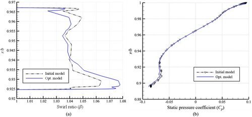
In addition, the optimum length of the chord in the hub was shorter than the midspan and tip section. This helped in reducing pressure loss in the boundary layer of the hub wall, which is shown in Figure 17(b). Static pressure at pre-swirl nozzle outlet was expressed as a pressure coefficient (C_P), and the low C_P means high static pressure at pre-swirl nozzle outlet which means less energy losses. 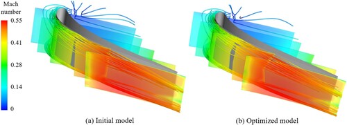(6) $C_P=\frac{p_s-p_{1s}}{\frac{1}{2}\rho {\mathrm{\Omega }}^2{r}^2}$(6) Figure 18 shows the flow structure near the hub, shroud, and nozzle wall. Contours of Mach number were colored on five axial planes, and 3D streamlines were included to illustrate the flow structure near the walls and tips on the freestream flow field. The streamlines and velocity distributions along the walls showed the similar trajectories until they reach the trailing edge, where the flow finally turns to the center position of flow path. Comparing the region near the trailing edge, it could be seen that the streamlines originated from the shroud showed a large part of the discharged flow enters the centre region of the flow path. In addition, this flow structure appeared more strongly in the optimized model. Due to the shape of trailing edge and midspan, the optimized model had a concentrated flow to the centre of flow path. This flow structure could minimize the energy losses of the flow into the receiver hole after the pre-swirl nozzle outlet. The discharge efficiency was maximized by minimizing the flow in the area exceeding the receiver hole diameter, and concentrating the flow to the center of the receiver hole.

Figure 18. Flow field and velocity streamlines near the wall.

5.2. Performance analysis

Through the improvement of the flow structure made by the optimization process, the optimized shape could have a more uniform flow distribution in the span-wise direction. The axial velocity contour of both models at the pre-swirl nozzle outlet is shown in Figure 19.

Figure 19. Axial velocity contour at the pre-swirl nozzle outlet.

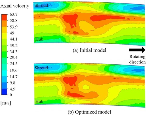
Since the same boundary conditions were applied to the system, an increase and uniform distribution of the axial velocity meant a decrease of the energy loss in the pre-swirl nozzle region. This can be said to be the effect of increasing the nozzle camber of the hub and shroud to reduce the flow path where the wall loss occurs, and extending the flow path by decreasing the camber of the midspan where has relatively small wall loss.

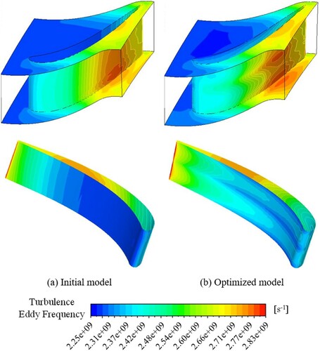
To analyze the energy transfer occurring around the different nozzle wall shapes, turbulence eddy frequency (ω) was studied. Turbulence eddy frequency is the rate at which turbulence kinetic energy (k) is converted into thermal internal energy per unit volume and time. (7) $\omega =\frac{ϵ}{k{\text{β}}^{\ast }}$(7) Where ε is turbulence dissipation rate and β* is a model constant. Turbulence energy is absorbed as internal energy by breaking the eddies gradually until it is converted into heat by viscous forces. The increase in internal energy is distributed between microscopic kinetic energy and microscopic potential energy. Also a mechanism of increasing internal energy in a closed system is the doing of work on the system such as mechanical form by changing pressure, volume, or by other perturbations.

As shown in Figure 20, around the pre-swirl nozzle region, optimized model showed high turbulence eddy frequency on the walls. The high turbulence eddy frequency caused high internal energy to the system, and this appeared as an increase in pressure at the system outlet which is one of the mechanical form of the internal energy.

Figure 20. Turbulence eddy frequency on the pre-swirl nozzle wall.

5.3. Off-design performance

All optimization processes were conducted for a single design point, at which the discharge coefficient of the optimized system was increased by about 2.57% over that of the initial system. In this study, to analyze the performance of various boundary conditions on the optimized model, performance analysis was conducted for six pressure ratio values and various different ambient air temperatures.

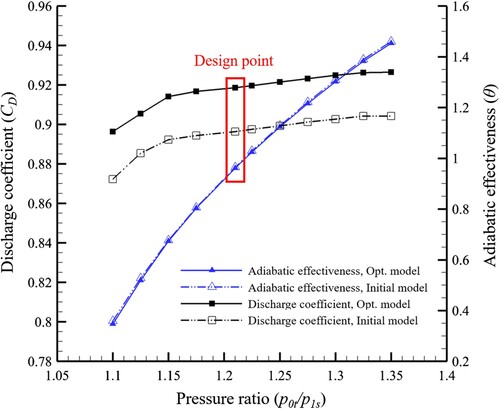
As shown in Figure 21, compared with the initial model, the optimized one showed an increased discharge coefficient at all pressure ratio conditions with negligible difference in adiabatic effectiveness. Based on these result, the mass flow rate of the optimized model could be the same as that of the initial one even when the pressure ratio is decreased by 1.19%.

Figure 21. Discharge coefficient and adiabatic effectiveness at various pressure ratio conditions.

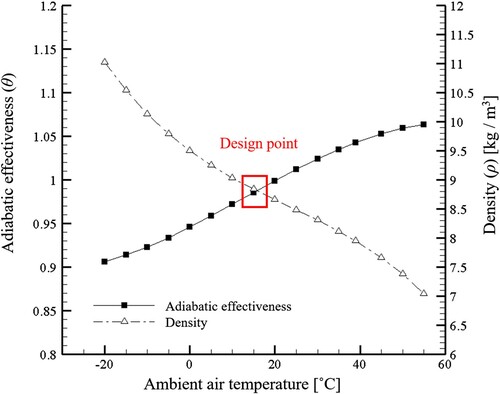
The performance of the pre-swirl system considering the ambient air temperature of the gas turbine is shown in Figure 22 and 23.

Figure 22. Discharge coefficient and non-dimensional mass flow rate at various ambient air temperature conditions.

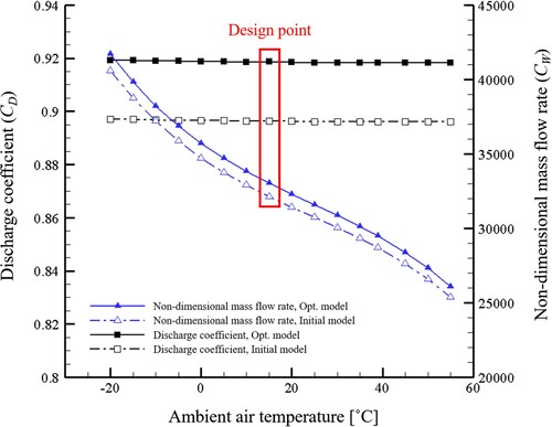
Figure 23. Adiabatic effectiveness and density at the optimized model outlet at various ambient air temperature conditions.

Normalized boundary conditions of the system for each ambient temperature is represented in Table 5.

Table 5. Pre-swirl system inlet total pressure at different ambient temperature.

Ambient temperature [°C]	−20	15	39	55
Normalized inlet total pressure	1.14	1	0.95	0.86
Normalized inlet total temperature	0.94	1	1.08	1.1

As ambient air temperature changed at a fixed system pressure ratio, the discharge coefficient of both the optimized and initial models remained almost constant. However, the actual mass flow rate tended to decrease at a high temperature due to the difference in air density. Furthermore, as the temperature increased and the density decreased, the adiabatic effectiveness tended to increase because of the increased air volume and circumferential velocity at the nozzle outlet. There were very small differences between the adiabatic effectiveness of the initial model and the optimized one for all the design points considered.

6. Conclusion

In this study, the geometries of a vane type pre-swirl nozzle were optimized using CFD and optimization methods. Performance analysis was also carried out for various boundary conditions. The design parameters for the vane were selected, and seven design variables were chosen through sensitivity analysis. OLHD and ALHD methods were applied to obtain test points for constructing a reliable surrogate model. The optimization was carried out until the difference between the candidate point predicted by the Kriging model and the CFD result was less than 0.5%, with a total of 76 test points being used.

The hub and shroud cross-sections of the optimized model had a smaller camber than for the initial one. In contrast, in the midspan section, the optimized vane had a larger camber than the initial one. In addition, as chord length of the vane was varied with span-wise direction, the trailing edge of the vane had a concave shape in that direction. This helped the pre-swirl system to have more concentrated flow to the center of flow path and uniform axial velocity distribution formed at the nozzle outlet, allowing a higher mass flow rate to the receiver hole. With the optimized model, the adiabatic effectiveness decreased slightly, whilst the discharge coefficient increased significantly.

In addition, the mechanism of increasing system pressure according to the change of system internal energy and turbulence eddy frequency near the walls was analyzed.

The off-design analysis using various boundary conditions such as pressure ratio and ambient temperature, the optimized model showed higher performance than the initial one for all conditions. It was found that the system discharge coefficient was increased by 2.57% without a large loss in adiabatic effectiveness, in the optimized model when compared to the initial one. The loss of adiabatic effectiveness will be minimized if the constraint on the circumferential velocity of the nozzle outlet can be kept tighter.

An optimization method and its process have been shown using CFD methodology. However, this study was conducted without experiments data for optimized model and temperature parameters. To improve the confidence of study, additional experiment for the optimized model and unsteady analysis will be conducted in the future study.

The authors believe that the optimization process proposed here would also be useful for designing pre-swirl systems of gas turbine engines.

Disclosure statement

No potential conflict of interest was reported by the author(s).

Additional information

Funding

This work was supported by Korea Institute of Energy Technology Evaluation and Planning (KETEP) and the Ministry of Trade Industry and Energy Korea (MOTIE) [grant number 2013101010170A].

References

- Ahmed, M. Y., & Qin, N. (2009). Comparison of response surface and Kriging surrogates in aerodynamic design optimization of hypersonic spiked blunt bodies. 13th International Conference on Aerospace Sciences and Aviation Technology, 13, 1–17. https://doi.org/https://doi.org/10.21608/asat.2009.23443
- Benim, A. C., Brillert, D., & Cagan, M. (2004). Investigation into the computational analysis of direct-transfer pre-swirl systems for gas turbine cooling. Proceedings of the ASME Turbo Expo 2004, 4, 453–460. https://doi.org/https://doi.org/10.1115/GT2004-54151
- Bricaud, C., Geis, T., Dullenkopf, K., & Bauer, H. J. (2007). Measurement and analysis of aerodynamic and thermodynamic losses in pre-swirl system arrangements. Proceedings of the ASME Turbo Expo 2007, 4, 1115–1126. https://doi.org/https://doi.org/10.1115/GT2007-27191
- Ciampoli, F., Chew, F. W., Shahpar, S., & Willocq, E. (2007). Automatic optimization of pre-swirl nozzle design. Journal of Engineering for Gas Turbines and Power, 129(2), 387–393. https://doi.org/https://doi.org/10.1115/1.2364194
- Da soghe, R., Bianchini, C., & D’Errico, J. (2018). Numerical characterization of flow and heat transfer in preswirl systems. Journal of Engineering for Gas Turbines and Power, 140(7), 071901. https://doi.org/https://doi.org/10.1115/1.4038618
- Didenko, R. A., Karelin, D. V., Levlev, D. G., Shmotin, Y. N., & Nagoga, G. P. (2012). Pre-swirl cooling air delivery system performance study. Proceedings of the ASME Turbo Expo 2012, 4, https://doi.org/https://doi.org/10.1115/GT2012-68342
- Ditmann, M., Geis, T., Schramm, V., Kim, S., & Wittig, S. (2002). Discharge coefficients of a pre-swirl in secondary air system. Journal of Turbomachinery, 124(1), 119–124. https://doi.org/https://doi.org/10.1115/1.1413474
- Fonseca, C. M., & Fleming, P. J. (1993). Genetic algorithms for multiobjective optimization: Formulation, discussion and generalization. 5th International Conference on Genetic Algorithms, 93, 416–423.
- Javiya, U., Chew, J., & Hills, N. (2011). A comparative study of cascade vanes and drilled nozzle design for pre-swirl. Proceedings of the ASME 2011 Turbo Expo, 5. https://doi.org/https://doi.org/10.1115/GT2011-46006
- Javiya, U., Chew, J. W., Hills, N. J., Zhou, L., Wilson, M., & Lock, G. D. (2012). CFD analysis of flow and heat transfer in a direct transfer preswirl system. Journal of Turbomachinery, 134(3), 031017. https://doi.org/https://doi.org/10.1115/1.4003229
- Karabay, H., Chen, J.-X., Pilbrow, R., Wilson, M., & Owen, M. (1999). Flow in a “cover-plate” preswirl rotor-stator system. Journal of Turbomachinery, 121(1), 160–166. https://doi.org/https://doi.org/10.1115/1.2841225
- Kim, J., Kang, Y. S., Kim, D., Lee, J., Cha, B. J., & Cho, J. (2016). Optimization of a high pressure turbine blade tip cavity with conjugate heat transfer analysis. Journal of Mechanical Science and Technology, 30(12), 5529–5538. https://doi.org/https://doi.org/10.1007/s12206-016-1121-6
- Kim, D., Kim, J., Lee, H., & Cho, J. (2017). Effect of splitter location on the characteristics of a vane-type pre-swirl system. Journal of Mechanical Science and Technology, 31(3), 1267–1274. https://doi.org/https://doi.org/10.1007/s12206-017-0225-y
- Kim, D., Lee, H., Lee, J., & Cho, J. (2018). Design and validation of a pre-swirl system in the newly developing gas turbine for power generation. Proceedings of the ASME Turbo Expo 2018, 5B, V05BT15A027. https://doi.org/https://doi.org/10.1115/GT2018-76255
- Kusbeci, M. E., & Chew, J. W. (2018). Assessment of wall-modeled LES for pre-swirl cooling systems. Proceedings of ASME Turbo Expo 2018, 5B, V05BT15A004. https://doi.org/https://doi.org/10.1115/GT2018-75112
- Lee, S., Lee, S., Kang, Y., Rhee, D., Lee, D., & Kim, K. (2013). A study on reliability of Kriging based approximation model and aerodynamic optimization for turbofan engine high pressure turbine nozzle. Journal of Fluid Machinery, 16(6), 32–39. https://doi.org/https://doi.org/10.5293/kfma.2013.16.6.032
- Lee, H., Lee, J., Kim, D., & Cho, J. (2018). Pre-swirl system design including inlet duct shape by using CFD analysis. Proceedings of the ASME Turbo Expo 2018, 5B, V05BT15A029. https://doi.org/https://doi.org/10.1115/GT2018-76323
- Lee, H., Lee, J., Kim, D., & Cho, J. (2019). Optimization of pre-swirl nozzle shape and radial location to increase discharge coefficient and temperature drop. Journal of Mechanical Science and Technology, 33(10), 4855–4866. https://doi.org/https://doi.org/10.1007/s12206-019-0926-5
- Lee, J., Lee, H., Kim, D., & Cho, J.. (2020). The effect of rotating receiver hole shape on a gas turbine pre-swirl system. Journal of Mechanical Science and Technology, 34(5), 2179–2187. https://doi.org/https://doi.org/10.1007/s12206-020-0439-2
- Liu, Y., Liu, G., Konh, X., & Feng, Q. (2016). Design and numerical analysis of a new type of pre-swirl nozzle. Proceedings of the ASME Turbo Expo 2016, 5A, V05AT15A013. https://doi.org/https://doi.org/10.1115/GT2016-56738
- Montgomery, D. C., Runger, G. C., & Hubele, N. F. (2009). Engineering statistics. John Wiley & Sons.
- Myers, R. H., Montgomery, D. C., Vining, G. G., Borror, C. M., & Kowalski, S. M. (2004). Response surface methodology: A retrospective and literature survey. Journal of Quality Technology, 36(1), 53–77. https://doi.org/https://doi.org/10.1080/00224065.2004.11980252
- Park, S. H., Yeo, H. G., & Rhee, S. H. (2019). Isothermal compressible flow solver for prediction of cavitation erosion. Engineering Applications of Computational Fluid Mechanics, 13(1), 683–697. https://doi.org/https://doi.org/10.1080/19942060.2019.1633688
- Pritchard, L. J. (1985). An eleven parameter axial turbine airfoil geometry model. Proceedings of the ASME 1985 International Gas Turbine Conference and Exhibit, 1, V001T03A058. https://doi.org/https://doi.org/10.1115/85-GT-219
- Ramezanizadeh, M., Nazari, M. A., Ahmadi, M. H., & Chau, K. W. (2019). Experimental and numerical analysis of a nanofluidic thermosyphon heat exchanger. Engineering Applications of Computational Fluid Mechanics, 13(1), 40–47. https://doi.org/https://doi.org/10.1080/19942060.2018.1518272
- Wilson, M., Pilbrow, R., & Owen, J. M. (1997). Flow and heat transfer in a preswirl rotor-stator system. Journal of Turbomachinery, 119(2), 364–373. https://doi.org/https://doi.org/10.1115/1.2841120