Numerical study of the effects of CO₂ gas in geothermal water on the fluid-flow characteristics in production wells

Abstract

In this study, we numerically investigated the effects of CO₂ gas in geothermal water and the scale deposition formed in the wellbore on the flow characteristics. Geothermal water that contains CO₂ gas has the potential to produce calcite scale deposits in the wellbore. To prevent scale formation, scale inhibitor is injected below the flash point in the wellbore, which is a challenging job. Therefore, using a wellbore simulator to predict the depth of flash commencement and the effects of scale deposition above the flash point on flow characteristics is important. In our numerical simulations, we changed the values of the CO₂ gas concentration to study its effect on the flow characteristics. The simulation results show that the presence of CO₂ increases the flash pressure relative to that of pure water. A higher CO₂ gas concentration in the water will initiate flashing at a lower depth than a lower CO₂ concentration. However, when the presence of scale deposits in the wellbore is taken into account, the calculated wellhead pressure is lower than that in a wellbore without scale deposition.

KEYWORDS:

• CO₂ gas
• scale deposition
• flashing depth
• numerical analysis
• flow characteristics

Nomenclature

Latin symbols

F	=	Flux (/m2 s)
G	=	A function
H	=	Specific enthalpy (J/kg)
K′	=	Equilibrium constant (-)
M	=	Mass rate (kg/s)
n	=	Mass of CO2 per unit mass (-)
P	=	Pressure (Pa)
T	=	Temperature (°C)
U	=	Specific internal energy (J/kg)
v	=	Specific volume (m3/s), fluid velocity (m/s)
V	=	Volume flux (m/s)
x	=	Steam quality (-)

Greek letters

α	=	A function
γ	=	Mass of CO2 per unit mass of fluid (-)
ϵ	=	Surface roughness of pipe (m)
μ	=	Dynamic viscosity (Pa s)
ρ	=	Density (kg/m)

Subscripts

c	=	Partial
ct	=	CO2 gas mass flow rate
E	=	Enthalpy
g	=	Gaseous phase
gc	=	CO2 in steam
gw	=	Steam phase in viscosity term
ℓ	=	Liquid phase
ℓc	=	CO2 in water
m	=	Mass
o	=	Standard condition
s	=	Steam
sc	=	Deposited scale
sat	=	Saturated condition
soln	=	Solution of CO2 in water
t	=	Total
w	=	Water
wh	=	Wellhead
wt	=	Water mass flow rate

1. Introduction

A high concentration of dissolved CO₂ gas in geothermal fluids is one of the main causes of calcite (CaCO₃) scale deposition in production wells. Some of the techniques available to overcome this problem include mechanical cleaning with a reamer, chemical inhibition, side tracking (deviation of the well), deepening of the well, changing the mode of well operation, and creating a new well design. The inhibition of scale deposits by the use of chemical products has gained importance both technically and economically, and seems to be one of the most promising approaches (Molina, 1995). This technique basically aims to prevent the formation of scale. To do so, a scale inhibitor is injected through a tube extending into the production well, which is a very challenging job for engineers. Before injecting the inhibitor, the engineers must know the precise location of the scale deposits; hence, the importance of the current study.

Calcite scale deposits are normally found on the wellbore surface above the flash point. When pure liquid water is present in the reservoir or in the bottom of the well during production, no problem arises in the pressure or temperature profiles in the wellbore when the water flows upwards. The liquid water begins to flash into steam at a certain depth, and a two-phase fluid flows from that point up to the wellhead. However, when the liquid water at the well bottom contains non-condensable gas (NCG), such as CO₂, the pressure and temperature profiles will shift to higher values as the fluid approaches the wellhead. In this situation, the operators must be careful when measuring the pressure and temperature at the wellhead because they could provide misleading interpretations of the downhole conditions if they fail to evaluate the CO₂ content in both the liquid and steam phases. An additional issue is that the presence of CO₂ in the liquid may cause calcite deposition in the wellbore, which is commonly found just above the flash point. The effect of calcite deposits in the wellbore is, however, a reduction in the pressure in the wellbore. Thus, opposite effects are observed from the above two issues, whereby the presence of CO₂ in the water causes an increase in the pressure, and calcite scale deposits will reduce the pressure. In practical applications, the presence and geometry of calcite deposition can be observed using a sinker bar (go-devil) or caliper logging tools, which are very costly. Alternatively, numerical simulation can be utilized to estimate the location and geometry of the calcite deposition. The calculated pressure and temperature at the wellhead can then be compared with the measured pressure and temperature at the wellhead, which involves much less cost. By varying the location and geometry of the simulated calcite depositions, the calculated and measured pressure and temperature at the wellhead can be matched to obtain the real conditions. Therefore, it is important to estimate the depth of the flash point below which the scale inhibitor should be injected via a coiled tube into the well.

The flashing depth at which water begins to generate steam depends on the saturation pressure corresponding to the fluid temperature at depth. However, the flash point of water containing CO₂ gas differs from that of pure water. Calcite scale is commonly found in wells that produce fluids with high concentrations of CO₂. As scale deposition proceeds in a well, it causes a decrease in the well’s mass flow rate. Consequently, the installed capacity also decreases due to a lack of steam production in the wells. When scale is formed in the wellbore, it should be removed either mechanically or by acidization. However, the formation of scale deposits can be avoided by injecting a scale inhibitor. From the technical and economic perspectives, the injection of an inhibitor seems to be the most reliable method of preventing scale formation in wellbores. Because calcite scale is normally located from the flash point in the wellbore to the wellhead, the scale inhibitor is injected below that point (Fujii, 1988). To design an effective inhibitor system, it is important to locate the depth at which flashing begins. Chemically, calcite scale deposition occurs when the geothermal water becomes saturated with calcite at the reservoir temperature. Once it becomes supersaturated with respect to calcite solubility as the water flashes, the temperature of the water is decreased.

Takahashi (1988) and Tanaka and Nishi (1988) performed wellbore simulations that featured the presence of CO₂ in geothermal fluid. The authors simulated the measured pressure and temperature profiles in production wells and attained good matching results between the measured and simulated profiles with respect to both pressure and temperature. However, the presence of CO₂ in the liquid water is usually accompanied by the formation of calcite deposits, which affects the flow in wellbores. Therefore, the effects of the CO₂ concentration in geothermal water as well as the reduced wellbore diameter due to scale deposition in the wellbore were examined in detail.

As an example, we consider the calcite scale deposition in Well MT-27 at the Momotombo geothermal field, Nicaragua. From 1996 to 1999, most of the shallow production wells at Momotombo, including Well MT-27, could not maintain wellhead pressure to produce the fluids. These problems were determined to be caused by the formation of calcite scale in the wellbore. To recover well productivity, the wells were mechanically cleaned and steam production resumed after the cleaning repair operations. The wellhead pressures and flow rates of Well MT-27 were measured from May to October in 2000 and in May 2000, just after mechanical cleaning had been performed in April 2000, at which time well deliverability was restored. The deliverability curve for Well MT-27 represented the well characteristics when there was no scale deposition in the wellbore. However, in the subsequent months from August to October, the well experienced decreases in both the wellhead pressures and flow rates with time, which was judged to be due to the formation of calcite scale in the wellbore (Khasani, 2005).

Satman et al. (1999) investigated the effects of the deposition of calcite on the inflow performance of geothermal wells that produce brine with CO₂ contents. The authors found that the rate of calcite scaling was inversely proportional to the square of the radial distance from the well. At a certain flow rate, the amount of calcite deposition around a well may be reduced by decreasing the pressure gradient near the well and/ or increasing the effective wellbore radius. Reservoir parameters such as reservoir pressure, wellbore flow pressure, permeability, and skin were considered to affect calcite deposition.

Haizlip et al. (2012) utilized a steady-flow wellbore model to evaluate the dynamic pressure and temperature profiles in two wells with different mass flow rates due to the presence of NCG. The authors concluded that the depth of gas breakout (bubble) in high gas wells can be estimated using the measured downhole pressure from dynamic surveys and calculating total pressure as equal to the liquid water pressure plus the gas pressure. However, variation in the gas content was not considered in their study. Using a wellbore model, variation in the CO₂ concentration was evaluated by Barelli et al. (1982) with respect to the pressure and temperature profiles in wells. These authors compared the simulated and measured pressure and temperature profiles and concluded that if the dissolved gases are neglected even at low concentrations, it is difficult to fit the pressure and temperature profiles and that, in many cases, there would be no well production at all. Moreover, the effects of scale deposition in the wellbore on wellbore flow were not considered in their study.

Molina (1995) discussed the problems caused by solid deposition in geothermal production wells and described methods to minimize these problems. Calcite, silica, and sulfide are the most common scaling minerals present in geothermal systems, and are found in the production casings and slotted liners of production wells. The author stated that the inhibition of scale deposits by the use of chemical products becomes important from both the technical and economic perspectives, and seems to be the most promising approach. The choice of scale inhibitor and the system used to inject it into the well are critical factors in this method.

Siega et al. (2005) described the calcite inhibition system already installed in two of the production wells affected by calcite deposition at the Mahanagdong geothermal field, Philippines. This downhole injection facility consisted of 2000m of a 1/4-in SS-316 capillary tubing, and the types of inhibitors used were polyacrylic acid and polymaleic anhydrides, both of which are acidic. In both wells, the depth of the flash point was determined to be deeper than 1650 to 1750 m, so the injection depth of the inhibitor was set to at least 100 m below this level. The simulator WELLSIM was used to estimate the flashing depth and the expected pump injection pressure. The authors reported that chemical inhibition was generally successful in reducing the rate of decline in the mass flow, with this rate being significantly reduced from an average of 4.0 kg/s-month to less than 0.5 kg/s-month in terms of total mass flow.

Rangel et al. (2019) reported chemical inhibition to be the most appropriate option for maintaining continuous well flow to the power plants at the Ribeira Grande geothermal field, Azores, Portugal over the past 25 years of exploitation. Every production well has been equipped with an inhibitor system that enables the injection of a chemical calcite inhibitor inside the well at a calculated depth, based on estimations of the depth of the flash point. Every six months, the system is removed from the well to inspect the degree of calcite deposition and evaluate the mechanical condition of the downhole tools.

Allan et al. (2019) developed a simple model for calcite scale in geothermal wellbores to evaluate the results of interventions and predict the amount of scale that would be encountered following these interventions. The model was implemented to evaluate Well NM12 at the Ngatamariki geothermal field, New Zealand. This well began operation in late 2014 with a capacity of 1050 t/h of two-phase fluid at minimum operating wellhead pressure. The flow of the well gradually started to decline in early 2017 but this rate accelerated over time. According to their model, the wellhead pressure with a flash point before the occurrence of scaling was 25 barg. A section of scale was introduced into the model by reducing the internal diameter, starting at the flash point and extending upwards. Two important parameters, the length and thickness of the scale, were changed to match the decline in the flow rate and wellhead pressure experienced by NM12. Different combinations of length and diameter could be used to match the NM12 performance. This wellbore simulation demonstrated that a significant amount of scale can build up before changes in flow rate are evident. However, the authors did not consider the variation of CO₂ in their study, which is an important factor to consider as it may change from time to time due to dynamic processes in the reservoir. A more comprehensive modeling of scale deposition study was conducted by Abouie et al. (2017). They used a coupled geochemical and compositional wellbore simulator. The simulator was able to predict the deposition profiles of carbonate and sulphate scales in the wellbore. Some important parameters that affected the scale deposition included pressure, temperature, salinity, and pH value. However, this wellbore simulator was developed for petroleum application which was much different from geothermal application due to different in the field nature.

Renaud et al. (2019a) introduced deep borehole heat exchangers (DBHE), a technology for harvesting heat from unconventional geothermal resources that do not require fluid exchange between the subsurface and wellbore. Using computational fluid dynamics (CFD) in a 30-year simulation, the authors investigated the thermal effects and heat recovery of a hypothetical DBHE and two wellbore designs. They demonstrated that the output temperature was a function of the working fluid velocity and that the cooling perturbation near the well bottom increased radially as a function of the production time. The power output of the well was also calculated. In addition, this CFD simulation identified the flow patterns in the wellbore. In the Krafla geothermal field in Iceland, this technology was combined with the organic Rankine cycle to convert thermal energy into electricity (Renaud et al., 2019b). Other applications of CFD models for real cases can also be found in Ez Abadi et al. (2020), Ramezanizadeh et al. (2019), Akbarian et al. (2018).

The aim of this numerical study was to comprehensively study flow characteristics, including the effects of dissolved gas in the geothermal water, scale deposition, and feed-point conditions. By numerically determining the depth of the flash point, the depth at which the chemical inhibitor should be injected can be precisely determined. In addition, other useful results that can be obtained from this study, including the wellhead pressure and temperature, the well productivity, and the power output, which are required for resource management.

2. Theory

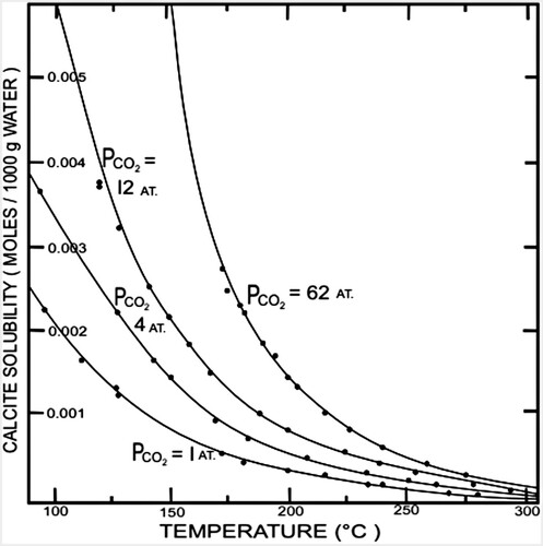
Geothermal waters are generally close to calcite saturation (Arnórsson, 1978). High CO₂ fluids that are normally also rich in Ca are more likely to deposit calcite than fluids poor in CO₂ (Mroczek & Graham, 2001). Chemically, calcite scale deposition occurs when geothermal water saturated with calcite at the reservoir temperature become supersaturated with respect to calcite solubility, which increases as temperature decreases, as shown in Figure 1. We can see that for the same temperature, the solubility of calcite is higher at the high partial pressure of CO₂. Practically speaking, to avoid calcite deposition, the operating temperature should be set as low as possible and careful treatment must be considered when the water is subjected to a higher-temperature environment.

Figure 1. The solubility of calcite in water up to 300°C at various partial pressures of carbon dioxide (Reproduced from Ellis, 1959).

2.1. Calcite saturation in geothermal reservoir water

Geothermal-fluid-chemistry field data indicate that water at depth in reservoirs is close to being saturated with calcite, as reported by White et al. (2000), Durak et al. (1993), Mercado et al. (1989) and Vaca et al. (1989).

The solubility of calcite can be expressed as follows (Arnórsson, 1978): (1) $\text{CaC}{\text{O}}_{3,s}+2{\text{H}}^{+}=\text{C}{\text{a}}^{2+}+\text{C}{\text{O}}_2+{\text{H}}_2\text{O},$(1) with the equilibrium constant K_s’ expressed as: (2) $\frac{(\text{C}{\text{a}}^{2+})}{{({\text{H}}^{+})}^2}\cdot {\text{P}}_{\text{C}{\text{O}}_{\text{2}}}=K_s^{\mathrm{\prime }},$(2) where the terms in the parentheses indicate activity.

The ratio of (Ca²⁺)/ (H⁺)² in geothermal water varies with temperature because it is controlled by the solubility of calcite and other minerals. As we can see in Equation (2), a certain supply of CO₂ is required to maintain a sufficient CO₂ partial pressure for calcite saturation. If the amount of CO₂ introduced to the system is greater than that required for calcite saturation, CO₂ will behave as a dissolved component.

2.2. Effects of flashing on calcium carbonate saturation

Flashing leads to a reduction in the CO₂ partial pressure due to the transfer of CO₂ into the steam phase. At any particular temperature, a decrease in the CO₂ partial pressure results in a decrease in the solubility of calcium carbonate in aqueous solution. Arnórsson (1978) described the changes in fluid characteristics that accompany the flashing of geothermal waters with respect to the state of calcite saturation, whereby the degassing of CO₂ leads to increases in the pH and carbonate ion concentration.

If the flashing process is adiabatic, the degree of supersaturation typically reaches a maximum after cooling by 10–40°C. The degree of supersaturation depends on the flashing level, salinity, and initial temperature (Arnórsson, 1981). The higher is the salinity of the water and the lower is the temperature, the higher is the degree of maximum supersaturation. When the supersaturation is at maximum, the flashed water has been degassed with respect to CO₂. Further flashing, which leads to cooling of the water, will cause a decrease in the degree of supersaturation because the solubility of calcite increases with decreasing temperature.

Generally, phase separation contributes very little to the calcium carbonate supersaturation relative to adiabatic flashing. The reason for this is that only limited steam formation is required to quantitatively degas geothermal waters with respect to CO₂. This is because in most geothermal wells, even heat flow from a rock formation can contribute to the elevated discharge enthalpy, but it has little effect on boiling. As such, in most cases, the process of fluid flow in the wellbore is assumed to be adiabatic. After flashing occurs in the wellbore, the process that plays the most important role in the boiling of the flowing water is the pressure drop, which is mainly due to the loss in the acceleration component by the flow of steam. This extensive boiling continues as the fluid approaches the wellhead.

3. Numerical modeling

3.1. Governing equations

In this numerical study, the fluid in the reservoir is assumed to be a single-phase liquid containing CO₂ gas. For this study, the mass and energy conservation equations for water, steam, and CO₂ in the fluid flow of the wellbore were taken from those reported by Sutton (1976), and can be found in the Appendix. The basic equations used both for single-phase and two-phase flows in the wellbore are mass and momentum equations, as follows: (3) $\frac{dM}{dl}=0,$(3) (4) $\mathrm{\Delta }{P}_t-\{\mathrm{\Delta }{P}_a+\mathrm{\Delta }{P}_h+\mathrm{\Delta }{P}_f\}=0,$(4) where M is the total mass flow (kg/s); l is the depth coordinate (m); ΔP_t is the total pressure drop (Pa); ΔP_ais the pressure drop due to acceleration loss (Pa); ΔP_h is the pressure drop due to potential loss (Pa); ΔP_f: is the pressure drop due to friction loss (Pa)

When a single-phase fluid flows up a vertical pipe, the fluid pressure drop can be expressed by rearranging Equation (5) as follows: (5) $\mathrm{\Delta }{P}_t=\mathrm{\Delta }{P}_h+\mathrm{\Delta }{P}_a+\mathrm{\Delta }{P}_f.$(5) The pressure loss components can be written as follows: (6) $\begin{array}{rl}\mathrm{\Delta }{P}_h& =\rho .g.\mathrm{\Delta }L,\end{array}$(6) (7) $\begin{array}{rl}\mathrm{\Delta }{P}_a& =G^2(v_1-v_2),\end{array}$(7) (8) $\begin{array}{rl}\mathrm{\Delta }{P}_f& =\frac{\lambda }{2D}\frac{G^2}{\rho }\mathrm{\Delta }L,\end{array}$(8) where G is the mass velocity (kg/m² s); v₁, v₂ is the specific volume of fluid at the inlet and outlet of an interval ΔP (m³/kg); λ is the friction factor (-); ΔL is the length of small increment (m); ρ is the fluid density (kg/m³)

The friction factor, λ, is given by Swamee and Jain (1976): (9) $\lambda =\frac{64}{Re}\text{if}\text{Re}<2100,$(9) (10) $\lambda =\frac{0.25}{{\left[{\log }_{10}\left(\frac{\epsilon /D}{3.7}+\frac{5.74}{{Re}^{0.9}}\right)\right]}^2}\text{if}\text{Re}>2100,$(10) where Re is the Reynolds number and ϵ is the pipe roughness.

When two-phase flow is considered, the flow of liquid water and steam are generally considered separately, and then the equations for the two phases are combined by solving the governing equations simultaneously. The main objective of this calculation is to determine the pressure drop in the wellbore. In this study, we used the method proposed by Orkiszewski (1967). We determined all the thermodynamic properties of the fluid using the sub-program PROPATH. Some basic correlations among the flow parameters include the mass fraction of steam, mass velocity, void fraction, and velocity ratio.

The mass fraction of steam, x, which is sometimes referred to as the dryness, is given as: (11) $x=\frac{M_g}{M_t}=\frac{M_g}{M_g+M_l}$(11) where the subscripts g and l indicate steam (gas) and liquid, respectively.

The mass velocity, G, is defined as follows: (12) $G=\frac{M_t}{A}=\frac{M_g+M_l}{A_g+A_l},$(12) where A is the cross-sectional area of the well and A_g and A_l are the cross-sectional areas occupied by steam and liquid, respectively.

The void fraction, α, is often defined as the ratio of the gas volumetric flow rate to the total flow rate: (13) $\alpha =\frac{Q_g}{Q_g+Q_l},$(13) where Q_g and Q_l are the volumetric flow rates of steam and liquid, respectively.

The velocity ratio, K, is defined as: (14) $K=\frac{u_g}{u_l}$(14) where u_g and u_l are the average velocities of the steam and liquid, respectively, which are defined as follows: (15) $\begin{array}{rl}{u}_g& =\frac{Q_g}{A_g}=\frac{M_g}{A_g}\frac{1}{{\rho }_g},\end{array}$(15) (16) $\begin{array}{rl}{u}_l& =\frac{Q_l}{A_l}=\frac{M_l}{A_l}\frac{1}{{\rho }_l}.\end{array}$(16) The characteristics of two-phase flow differ from those of single-phase flow, the main difference being the respective existence or absence of interfaces. When a fluid flows together with its steam in a pipe, each phase occupies a portion of that pipe’s cross-sectional area. An understanding of the flow patterns is important at the design stage, because in particular situations the fluid cannot flow in certain regimes. For example, it is not desirable for a steam turbine to be subjected to large slug of water, so the pipeline design must not include a slug regime. In this study, the flow regimes are classified into bubble, slug, transition, and mist, as described by Orkiszewski (1967).

3.2. Model and calculation methods

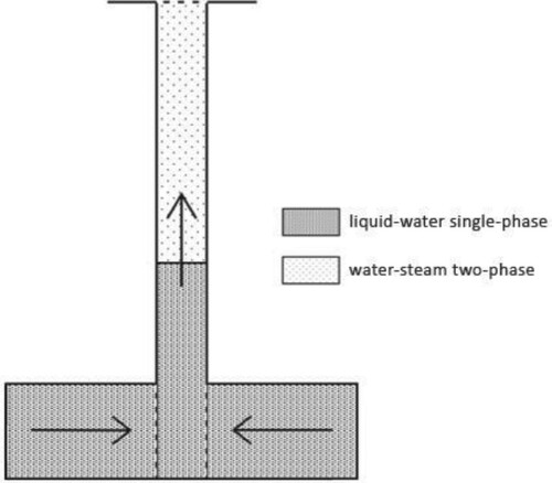
The wellbore model used in this study is the same as that reported by Khasani (2005), as shown in Figure 2, except that we did not include the reservoir model. The governing equations for this model are presented in Section 3.1 above. In geothermal wells that operate from a hot water reservoir, the flow of fluid starts at the depth at which the pressure is higher than the saturation pressure, which corresponds to the local temperature. That is, the fluid flows in a single-phase, as illustrated in Figure 2. Two-phase flow in a well begins where the fluid pressure reaches saturation pressure and the liquid starts flashing to form steam.

Figure 2. Schematic diagram of the wellbore model (From Khasani, 2005).

Based on all the thermodynamic variables described in Equations (A1) to (A36), we determined the pressure loss for the liquid and gaseous phases to obtain profiles of the pressure and temperature in the wellbore. We divided the wellbore into small grids from the bottom to the top of the wellbore, with each pair of grids having a pressure increment of ΔP and a length increment of ΔL. The input data for calculation included the initial pressure, P_o, initial temperature T_o, mass flow rate, M_t, well diameter, D, well length, L, pipe roughness, ϵ, and CO₂ gas content, n_c. The calculation was performed from the well bottom to the top of the wellbore. We determined the flash starting pressure, which consists of the saturation pressure and partial pressure of CO₂. The momentum equation was solved iteratively for small increments of ΔP at fixed increment lengths in the wellbore, ΔL. When the calculated pressure for a certain grid was greater than that of the flash starting pressure, the fluid is in single-phase condition, and the fluid properties in this grid were determined based on this calculated pressure and T_o. When the calculated pressure was lower than that of the flash starting pressure, the fluid is in two-phase condition, and the temperature of a certain grid was calculated using Equation (A9). Other parameters were calculated using the appropriate equations. The fluid properties were calculated based on the temperature. Details for calculating the fluid-flow parameters in the wellbore are presented in Figure 3.

Figure 3. Flow chart of the parameter calculations in the wellbore.

3.3. Input parameters and boundary conditions

Table 1 shows a summary of the wellbore geometry used in this study, for which the mass flow rate including CO₂ gas was 50 kg/s. We evaluated the CO₂ content (n_c) at 0, 0.5 and 1 wt% in the liquid water. The pressure and temperature at the well bottom, as the boundary conditions, were 75 bar and 260°C, respectively. These values were selected as those at which calcite deposition occurred in the wellbore. The presence of scale deposits in the wellbore is expressed by the reduction of the well diameter from the flash point to a specific depth.

Table 1. Wellbore parameters.

Parameter (unit)	Value
Well-bottom pressure (bar)	75
Well-bottom temperature (°C)	260
Mass flow rate (kg/s)	50
Well diameter (m)	0.2
Well length (m)	1500
Pipe roughness (m)	4.6 × 10^−5

4. Results and discussion

4.1. Effect of CO₂ gas content on the pressure and temperature profiles

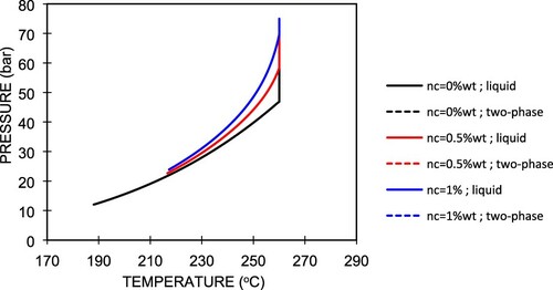
Figure 4(a,b) show the simulated pressure and temperatures profiles for different CO₂ contents, the respective phase diagram of which is shown in Figure 6. Tanaka and Nishi (1988) reported field data for 16 wells at Nigorikawa, in which the maximum CO₂ content was 2.8 wt% at the well bottom. In this study, we used three different gas content values, n_c= 0, 0.5, and 1 wt%. In Figure 4(a), we can see that when the CO₂ gas is in the single-phase liquid, the different amounts of CO₂ exhibit similar pressure profiles on the lowermost part of the curves, which is also evident in Figure 5(a). The pressure gradients increase linearly. Degassing of CO₂ occurs after the pressure in the wellbore reaches the flash starting pressure, which equals the sum of the saturation pressure and partial pressure of CO₂. This process occurs in such a way that CO₂ degases and then the liquid water starts to generate steam when the saturation pressure is reached. The decrease in the pressure gradient starts from that point and proceeds nonlinearly. The decrease rate of pressure at 0 wt% CO₂ is the highest when the fluid flows upwards in the wellbore and becomes smaller at higher initial CO₂ concentrations in the liquid phase. This is because the partial pressure of the CO₂ gas is proportional to n_ℓ and n_g and contributes to the total pressure.

Figure 4. Pressure (a) and temperature (b) profiles for different CO₂ gas contents.

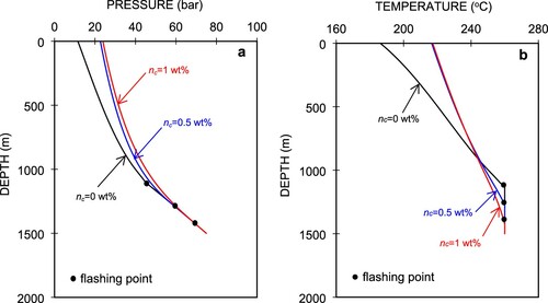
Figure 5. Pressure gradient (a) and temperature gradient (b) of fluid flow in the wellbore.

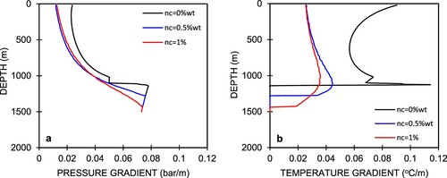
Figure 6. Phase diagram of the geothermal fluid in the wellbore for different CO₂ gas contents.

From the well bottom to the flash point, we can see that the pressure profile decreases linearly with a higher gradient. This indicates that the pressure drop is mainly due to elevation (gravitational component), which is greatly affected by a higher liquid water density. Once flashing starts, the liquid water changes into steam then water–steam two-phase flow continues upward to the wellhead. Because the density of this two-phase flow decreases as the fluid flows upward, the pressure drop due to the gravitational component becomes smaller, which results in the lower pressure gradient. In this section, the pressure gradient follows a quadratic trend because the pressure drop component due to acceleration from the steam phase becomes more dominant.

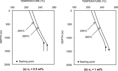
Figure 4(b) shows the simulated temperature profiles in the wellbore, in which we can see that the temperature starts to decrease once the fluid starts flashing, and the higher CO₂ content means the flashing depth is lower. Thermodynamically, the lower temperature at the uppermost area of the temperature profile for 0 wt% CO₂ in Figure 4(a) is due to the lower saturation pressure. In this study, the flashing depth was calculated to be 1130 m for pure water (n_c = 0 wt%), and 1270 and 1430 m for 0.5 wt% CO₂ and 1 wt% CO₂, respectively. An increase in the CO₂ content is also followed by an increase in the wellhead pressure, P_wh. The corresponding P_wh values for 0 wt% CO₂, 0.5 wt% CO₂, and 1 wt% CO₂ are 11.5, 22.7, and 23.9 bar, respectively. The temperature gradients also differ with the pressure gradients, as shown in Figure 5(b). For a single-phase liquid from the well bottom, the temperature gradients are zero. At the flash point, the sudden increase in the temperature gradients indicate that the thermodynamics properties have changed drastically from single-phase liquid to a two-phase condition. The temperature gradients are nonlinear with depth as fluid flow approaches the wellhead.

From Figure 6, it can be seen that for all CO₂ gas contents at high pressure and temperature, the fluid is in the single-phase liquid form. They only differ where the fluid starts boiling in the wellbore. For high CO₂ gas contents, e.g. 1 wt%, the fluid starts boiling at the higher pressure for the same temperature and vice versa. Below this saturation pressure, the fluid is in two-phase water–steam flow. A lower pressure corresponds to a lower temperature for the same CO₂ gas content.

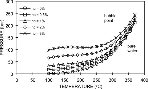
To explain the physics of the fluid flow in a wellbore containing different CO₂ gas contents, as illustrated in Figure 6, the boiling (bubble) point curves for different CO₂ concentrations, as shown in Figure 7, are useful. We note that the boiling (bubble) point curves are strongly affected by the CO₂ concentration. Recalling Equation (A13), where $P_c=P-P_{sat}(T)$, this means that the saturation (boiling) pressure of pure water depends on the partial pressure of CO₂. In the case of a single-phase liquid, because there is no CO₂ in the gas phase, we can directly apply the above correlation. For example, as shown in Figure 7, at a temperature of about 300°C, the pure water ($n_c=0,P_c=0$) boils at a pressure of 8.5 bar ($P=P_{sat}(T)$). For the same temperature, when 3 wt% of CO₂ is present in the water, the water will boil at the same saturation pressure but the CO₂ now provides an additional partial pressure of about 5.5 bar ($P_c$), which results in a total pressure (P) of about 14 bar. So, in this study, we find that the fluid starts to flash or boil at a higher pressure at a higher CO₂ concentration at the same temperature at the well bottom, as shown in Figure 4(a,b).

Figure 7. Phase diagram of water–carbon dioxide system (Adapted from Tanaka & Nishi, 1988).

In the case of a two-phase fluid, because the amount of CO₂ in the liquid phase is small, at the same temperature, the specific volume of the liquid phase, v_ℓ, is assumed to be equal to that of water, v_w. Considering that for a fixed temperature the molar ratio of CO₂ in the liquid phase is proportional to the partial pressure of CO₂ in the gaseous phase, we know that n_ℓ = n_c. In this condition, the total pressure follows Equation (A16),$P_{wtb}=P_{sat}(T)+n_c/\alpha (T)$ whereby it depends on the amount of CO₂ and the temperature. In Figure 4, we can see that the presence of CO₂ gas has significant effects, i.e. it increases both the pressure and temperature at the wellhead relative to that with pure water. The increase in CO₂ gas from 0.5 wt% to 1 wt% seems to have no significant effect on the pressure (6%) and temperature (0.3%) increases.

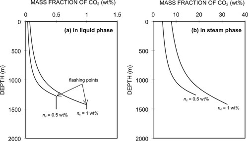
Figure 8(a,b) show the simulated CO₂ gas concentration profiles (in wt%) in the liquid and steam phases, respectively, for which we used two values of CO₂ gas concentrations at the well bottom, i.e. 0.5 and 1 wt%. These values were compared in both the liquid and steam phases as they moved up the wellbore to the wellhead. We can see that below the flash point, the CO₂ content in the liquid remains constant. This is because the amount of CO₂ as an NCG is present in water with a constant flow rate. Once flashing starts, the concentrations of CO₂ gas in the gas phase are much larger than those in the liquid phase, and the CO₂ content decreases as the fluid flows upwards in the wellbore. This is because the fluid temperature decreases from the flash point upwards in the wellhead. Consequently, the constant α(T) changes according to Equation (A10) and affects the CO₂ concentrations in both the liquid and steam phases. For n_c = 1 wt%, n_g = 8 wt% at the wellhead. This value is relatively high compared with that reported at the Momotombo field, which ranged between 1 and 4 wt%. This may be caused by the different well lengths or different pressures and temperatures at the well bottom. These parameters may result in different flashing depths, with the further implication that the mass fractions of the steam phase at the wellheads of both wells differ significantly.

Figure 8. Distribution of CO₂ concentrations in liquid (a) and steam (b) phases.

4.2. Effects of well-bottom temperature on flashing point depth

Figure 9 shows the pressure distributions in the wellbore for the different fluid temperatures at the well bottom for the two CO₂ concentrations, (a) n_c= 0.5 wt% and (b) n_c = 1 wt%. A 10°C decrease in the well-bottom temperature from 260°C to 250°C causes a decrease in the wellhead pressure (P_wh) of 3.56 bars for n_c= 0.5 wt% and 3.60 bar for n_c = 1 wt%. The pressure profiles are identical from the well bottom (1500 m) to a depth of about 1280 m for n_c = 0.5 wt% and 1420 m for n_c = 1 wt%. This is because the liquid phases remain the same from the well bottom up to those depths, which are clearly identified in the temperature profiles shown in Figure 10. From the figure, we can see that for the higher CO₂ content (n_c = 1 wt%), the 10°C temperature decrease from 260°C to 250°C, the flashing level shifts upwards by 77 m from 1426 m to 1349 m. For the lower CO₂ content (n_c = 0.5 wt%), the flashing depth shifts by 85 m. This is because the lower temperature corresponds to a lower saturation pressure. At the same flow rate, the flash point occurs at a shallower level for a lower saturation pressure.

Figure 9. Pressure profiles in the wellbore for different well-bottom temperatures and CO₂ concentrations.

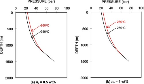
Figure 10. Temperature profiles in the wellbore for different well-bottom temperatures and CO₂ concentrations.

4.3. Effects of CO₂ gas content and scale deposition on flow characteristics

4.3.1. Scale deposition found in the field

Care should be taken when interpreting pressure profiles in the wellbore due to the presence of CO₂. This is because the presence of CO₂ causes calcite scale deposition in the wellbore. If data are available for the CO₂ gas contents in both the steam and water and the pressure in the wellbore, the wellbore analysis should consider the effect of the presence of CO₂ in the fluid and the scale. To date, most numerical studies (Barelli et al., 1982; Haizlip et al., 2012; Takahashi, 1988 & Tanaka & Nishi, 1988) have not considered the effect of scale deposition and the consequent a reduction in the wellbore diameter.

Fujii (1988) reported the calcite scale deposition in production wells at Nigorikawa, Hokkaido, Japan, as shown in Figure 11. Based on a caliper survey in the production wells, he found out that calcite scale had mainly formed along the wellbore from just above the flashing commencement point. The scale deposits in the shallow area were negligible. In this numerical study, we assumed the formation of scale of constant thickness and a fixed length of deposition. Considering the scale deposits in the wells shown in Figure 11, the length of the scale deposition was 200 m from the flash point with a constant thickness of 3 cm. In other words, the well diameter was assumed to have been reduced from 0.2 m to 0.194 m for depths from 1270 m to 1170 m. Other parameters are provided in Table 1. CO₂ contents (n_c) of 0 and 0.5 wt% were also used.

Figure 11. Calcite scale deposition in production wells at the Nigorikawa geothermal field, Japan (Reproduced from Fujii, 1988).

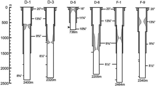
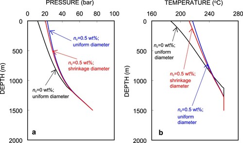
Figure 12(a,b) show the simulated pressure and temperature profiles, respectively, in the wellbore for different CO₂ gas contents in the fluid. The wellhead pressures for three conditions, i.e. (1) pure water (n_c= 0 wt%) and uniform diameter (case-1), (2) with n_c= 0.5 wt% with uniform diameter (case-2), and (3) with n_c= 0.5 wt% with a scale length of 200 m and thickness of 3 cm (case-3), were 11.5, 22.7, and 20.6 bar, respectively. The results for the case without any scale deposition and with CO₂ gas (case-1) shows the lowest P_wh (11.5 bars). This is because there is no additional partial pressure in the fluids. The presence of 0.5%wt CO₂ resulted in the highest P_wh increase at 22.7 bars or 97.4%, as indicated by case-2. The curves with CO₂ and wellbore diameter reduction (case-3) shows a lower P_wh than the curve without scale deposition (case-2). This indicates that by introducing scale deposition to the wellbore, the well diameter will be reduced and a greater pressure drop will occur in the wellbore. For the given scale-deposition geometry (length of 200 m and thickness of 3 cm), the pressure decreased at the wellhead by about 20.6 bars or 9% from that obtained with the uniform diameter and n_c= 0.5 wt% case. Therefore, scale deposition should be taken into account to obtain more reliable results with respect to the decrease in P_wh. At the same flow rate and CO₂ content, a reduction of the well radius due to scale-deposition results in a decrease in the wellhead pressure. This is mainly caused by larger pressure drops due to acceleration and friction components in the scale-deposited section of the well compared to that without scale. The temperatures at the wellhead also shows the lowest value for case-1 in Figure 12(b).

Figure 12. Pressure (a) and temperature (b) profiles in the wellbore for different CO₂ (n_c) gas contents and well-diameter reductions.

4.3.2. Effects of reduction of well diameter by scale deposition on pressure and temperature profiles in the wellbore

The field measurement of the scale deposition in the wellbore, as shown in Figure 11, indicates that scale deposits vary in length and thickness. Thus, it is important that wellbore flow analyses consider the presence of calcite deposits and examine the effects of the dimensions of the scale to gain a better understanding of the flow characteristics. As such, in our simulations, we considered some combinations of scale-deposition length and reduction of the well diameter due to scale-deposition.

For this purpose, we fixed the scale-deposition length, L_sc and used different thicknesses of deposited scale, d_sc. The mass flowrate was kept constant at 50 kg/s. In this part of the study, L_sc was fixed at 200 m and three different d_sc values were used: 10.75, 4.75, and 3.75 cm, the resulting simulated pressure and temperature profiles of which are presented in Figure 13(a,b), respectively. In the figures, we can see that from the well bottom to a depth of 1250 m where the flashing starts, there is no difference in the pressure and temperature profiles. This is because of the amount of CO₂ dissolved in the liquid is small, so v_ℓ can be assumed to be equal to the specific volume of water, v_w. This contributes to both the pressure and temperature values.

Figure 13. Pressure (a) and temperature (b) profiles for different reductions in the scale-deposition diameter.

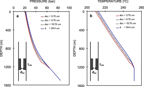
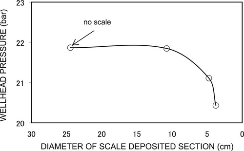
Introducing scale deposition from the level of the flash point produces different pressure and temperature profiles for various deposit thicknesses. The higher rates of decrease for both pressure and temperature within the length of the scale deposition is caused by the high pressure loss due to the friction and acceleration terms for a smaller diameter. The recovery of pressure and temperature from the end of the scale-deposition area upward is due to the decreased rate of pressure and temperature drop in this section. It can be observed that the pressures and temperatures at the wellhead are 20.43, 21.11, and 21.85 bar, and 209.2°C, 210.7°C, 212.3°C, respectively. These correspond to d_sc values of 0.0375, 0.0475, and 0.1075 m for the scale-deposited part. These values indicate that the smallest d_sc value (3.75 cm) yields the greatest decrease rate of the pressure and temperature in the scale-deposition section relative to other values. The largest d_sc value (10.75 cm) yields a wellhead pressure, P_wh, of 21.85 bar, which is close to that of P_wh without scale deposition (21.87 bar). This means that a scale-deposit diameter greater than 10.75 cm has no significant effect on the pressure profiles. However, once more scale has been deposited in the wellbore, a small change in the diameter of the scale deposit causes a significant P_wh change. As an example, a reduction of the diameter from 4.75 to 3.75 cm results in a decrease of P_wh by 0.68 bar. The corresponding temperature profiles are shown in Figure 13(b).

Figure 14 shows the P_wh changes for the different degrees of reduction in the scale-deposited diameter at the same mass flow rate and 200-m length of scale deposition. The smallest diameter of 3.75 cm yields only a P_wh decrease of 1.39 bar from the condition without scale deposition, which is probably due to the relatively low flow rate that corresponds to the high wellhead pressure. We note that there is a significant P_wh decrease for a diameter reduction to less than 10.75 cm, but this does not play an important role in the changes of P_wh if the reduced diameter remains greater than 10.75 cm.

Figure 14. Wellhead pressure with diameter of the scale-deposited section in a well.

4.3.3. Effects of the length of scale-deposited section on pressure and temperature profiles in the wellbore

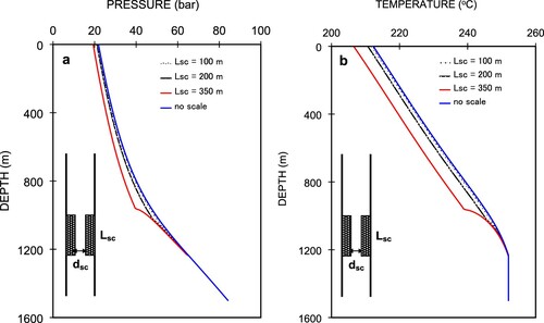
Next, we numerically evaluated the effects of the length of scale-deposited section in the wellbore on the pressure and temperature profiles. We varied the length of the scale deposition from a depth of 1200 m in the well between 100, 200, and 350 m. We used a well diameter of the scale-deposited section, d_sc= 4.75 cm, and a diameter of 0.2 m for the non-scale section. Figures 15(a,b) show the simulated pressure and temperature profiles, in which the wellhead pressures and temperatures are 21.66 bar, 21.11 bar, and 19.30 bar and 211.9°C, 210.7°C, and 206.5°C, respectively. These correspond respectively to L_sc = 100, 200, and 350 m.

Figure 15. Pressure (a) and temperature (b) profiles for different lengths of scale-deposited section.

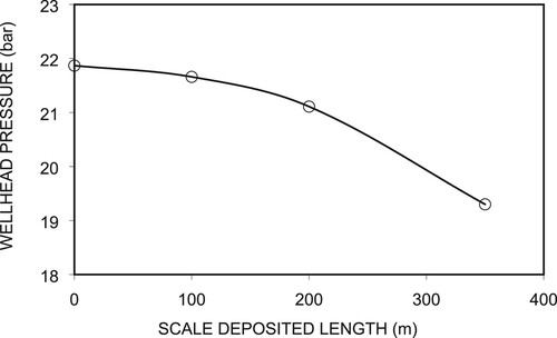
A longer deposition length yields a lower wellhead pressure. We can see that scale-deposited lengths of 100 and 200 m show no significant decrease in pressure in the deposited section compared to that of L_sc = 350 m. The pressure curve shows a discontinuity at a depth of 1000 m in the L_sc = 350 m curve at the shallower end of the scale-deposited section with respect to depth. In Figure 15, we can see that the pressure decrease rate for a scale-deposited length of 350 m is higher, and scale-deposited lengths of 100 and 200 m and that without scale deposition are roughly similar. This is because the fluid velocity is higher in the section with a smaller diameter. When the fluid leaves the scale-deposited section, the fluid velocity decreases as the diameter increases. Consequently, the pressure drops as the friction and acceleration values decrease. However, the scale-deposited length of 100 m shows no significant difference in its pressure profile compared to that of the well without scale. Figure 15(b) shows the corresponding temperature profiles. Due to friction, the 100-m length of deposited scale shows a relatively smaller pressure drop. Figure 16 shows the changes in P_wh values for scale-deposited sections with a diameter of 4.75 cm and different lengths at the same mass flow rate. In the figure, we can see that the decrease rate of the wellhead pressure is larger for a longer scale-deposited section, especially ones greater than 200 m. As the well-bottom pressures are the same for the four cases, as shown in Figure 15, this means that the total pressure drop between the well bottom and the wellhead increases with increases in the length of the scale-deposited section. The difference in wellhead pressure is caused by the additional pressure drop in the scale-deposited section. We can see that a scale-deposited section 100 m long is accompanied by a small additional pressure drop of approximately 0.5 bar, whereas that 350 m long experiences a more significant pressure drop of 2.5 bar. The decrease rate of P_wh follows almost linear correlation with respect to scale-deposited length.

Figure 16. Wellhead pressure change with scale-deposition length.

4.3.4. Numerical analysis of pressure and temperature profiles for Well C-2

Here, we consider the effect of calcite scale deposition on the pressure and temperature profiles of Well C-2 (Tanaka & Nishi, 1988). Fujii (1988) reported that the production of geothermal fluid decreases soon after a power plant becomes operational. This is due to the deposition of calcite scale in the production wells. To remove the scale in Well C-2, mechanical cleaning and acid treatment were performed repeatedly. However, as these measures did not fully resolve the scale problems, the injection of CaCO₃ scale inhibitor was adopted, which prevents the formation of the scale in the hot water of the production wells. The results of laboratory experiments using different chemicals revealed polyacrylic acid to be most effective. Since the adoption of the scale-inhibitor injection method, no scale has formed in the production wells except one instance when damage occurred to the tubing pipes through which the inhibitor is injected. To inject the scale inhibitor at the appropriate well depth below the flashing level, it is critical to evaluate the pressure and temperature profiles in the wellbore in the presence of CO₂ gas, which is the main cause of calcite deposition. Table 2 shows a summary of the field data obtained for calculating pressure and temperature.

Table 2. Summary of field data on Well C-2.

	Wellhead				Bottom hole
	Mass flow rate (t/h)
Mass fraction of CO2 (%)	Water	Steam	Total	Pressure (bar)	Depth (m)	Pressure (bar)	Temperature (°C)
1.0	148.0	10.0	158.0	21.1	1500	84.2	251

Here, a wellbore diameter of 9 5/8′′ (0.244 m) was used for the calculations. Numerical simulation was performed from the well bottom up to the wellhead with the wellhead conditions shown in Table 2. Figure 17(a,b) show the simulated pressure and temperature profiles.

Figure 17. Pressure (a) and temperature (b) profiles of Well C-2 with and without scale deposition.

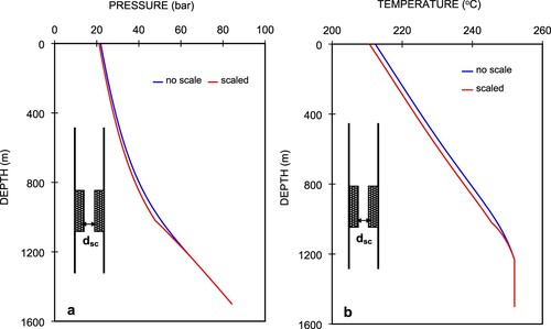
In Figure 17(a,b), the simulated pressure and temperature profiles for Well C-2 are based on 1 wt% CO₂ gas in the fluid with and without scale deposition in the well. For the case without scale, the pressure and temperature profiles are presented as blue lines at a pressure of 21.87 bar and a temperature of 212.3°C, respectively, at the wellhead. Smooth curves are observed in the pressure and temperature profiles. A number of simulations were performed by changing the combinations of scale-deposited length and diameter to realize a good match between the measured and simulated wellhead pressure of 21.1 bar. The combination of 200 m in length and a diameter of d_sc= 4.75 cm provided the best match by locating the scale-deposited section 200 m from the flash point at a depth of 1230 m up to 1030 m. The calculated pressure and temperature profiles are shown as red lines as shown in Figure 17. Both the pressure and temperature profiles show higher decrease rates starting from the flash point to the end of the scale-deposition section. These rates taper off as soon as the fluid leaves the scale-deposition section. This is because of the greater reduction in diameter due to scale deposition, which causes a higher fluid velocity for a constant mass flow rate. Consequently, the pressure drops as the friction and acceleration components increase.

4.3.5. Effects of scale deposition on deliverability curves

Based on the reduction of the well diameter due to scale deposition together with its length obtained from the preceding section (d_sc= 4.75 cm and L_sc=200 m), we evaluated the effects of scale deposition on well deliverability. We also used other Well C-2 field data listed in Table 2. The simulation was performed by varying the mass flow rate at the well bottom to obtain the corresponding wellhead pressures. Calculations were performed for wells with and without scale deposition and the results are presented in the form of deliverability curves. Figure 18 shows the deliverability curves for the well without scale (○) and with scale (□).

Figure 18. Deliverability curves for well with and without scale deposition.

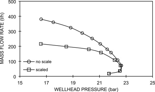
In Figure 18, we can see that at low flow rates, i.e. less than 70 t/h, and relatively high wellhead pressures, the curves with and without scale show no significant differences. Within this flow rate range, pressure drops in the wellbore are mainly due to potential drop because the wellbore is mostly occupied by liquid as the flashing point is located at a shallower level. Hence, the pressure drop is insensitive to a reduction in the well diameter. As the wellhead pressure decreases, the increase rate of the mass flow for the curve without scale is greater than that with scale. In this condition, the pressure drops due to friction and acceleration increase due to the reduction in the well diameter. At the same mass flow rate, the wellhead pressure of the well with scale deposition is lower than that without scale. At a given lower wellhead pressure range, the mass flow rate of the well with scale is also lower than that without scale.

At the same mass flow rate, for example 200 t/h, the presence of scale deposits in wellbore causes a higher fluid velocity along the scale-deposited section, as compared with that without scale. This leads to an increase in pressure drop due to acceleration and friction. As such, the wellhead pressure should be lower for a well with scale deposition because the well bottom pressures are the same for both cases. On the other hand, at the same wellhead pressure, for example at 19 bar, the presence of scale deposits in a wellbore results in a lower mass flow rate. In this scenario, we have two cases with the same pressure drops in the wellbore as the well-bottom pressures are the same. By applying Darcy’s equation and the principle of mass flow rate continuity, with the same pressure drop in the wellbore, the smaller is the diameter of the well with scale deposition, the lower will be mass flow rate, as shown in Figure 18.

5. Conclusions

Numerical simulations of wellbore flow to examine the effects of the CO₂ content in the geothermal fluid and scale deposition in the well on the pressure and temperature profiles in the wellbore and the well characteristics has been successfully performed in this work. This study is substantially important since it can be a tool for providing significant information in designing the inhibition technique to prevent the calcite scaling in the wellbore. In order to get the reliable results, both CO₂ content in the geothermal fluid and the artificial calcite scale diameter and length are given to examine their effects on the fluid characteristics that will in turns affect the power output of the wellbore. The quantitative results are summarized as follows:

1. The presence of CO₂ will increase the flashing pressure in comparison to that of pure water. When geothermal fluid containing CO₂ is produced from wells, the fluid flashes at a deeper point when it contains a higher CO₂ concentration.

2. For a given CO₂ gas concentration in liquid water, a lower fluid temperature yields a shallower flash point in the wellbore. At the same fluid temperature, a higher CO₂ concentration results in a deeper flash point.

3. In the presence of CO₂, scale deposition in the wellbore must be taken into account in numerical analysis. This is because the formation of scale leads to a reduction in the wellbore diameter, which accelerates the pressure drop in the scale-deposited section.

4. To evaluate the effects of scale deposition on the pressure and temperature profiles in a wellbore, its dimensions (length and diameter) must be evaluated in detail. Keeping the length of the scale-deposited section constant, the wellhead pressure is lower for smaller scale-deposited wellbore diameters. With the same scale-deposited wellbore diameter, a longer scale-deposited length results in lower wellhead pressure.

5. The deliverability curves for wells with scale deposition show a lower mass flow rate than those without scale deposition for a given wellhead pressure. The difference in mass flow rates of the deliverability curves increases as the wellhead pressures decrease.

Future work recommendation

To obtain more reliable results, we recommend that pressure and temperature field data field data be obtained for flowing wells with high levels of NCG (CO₂) and calcite-deposited scale. Variations in the diameter of the well due to deposited scale can be evaluated in numerical simulations to generate more precise results. The use of a transient fluid-flow model for a well represents a much more challenging study. Available publications of the experimental correlations and thermodynamic models for CO₂ solubility can be coupled with the simulator to examine their accuracy. The concentration of Ca²⁺ (salinity) in fluid may significantly affect scale deposition, so this topic should also be addressed in future work.

Acknowledgements

The first author would like to acknowledge the second and third authors for their valuable discussions and their contributions toward improving the manuscript.

Disclosure statement

No potential conflict of interest was reported by the author(s).

Appendix

The mass and energy conservation equations for water, steam, and CO₂ for the fluid flow in a wellbore that were used in this study were those reported by Sutton (1976) as follows: (A1) $V_{\ell }/v_{\ell }+V_g/v_g=F_m,$(A1) (A2) $n_{\ell }{V}_{\ell }/v_{\ell }+n_g{V}_g/v_g=\gamma F_m,$(A2) (A3) $H_{\ell }{V}_{\ell }/v_{\ell }+H_g{V}_g/v_g=F_e$(A3) where V_ℓ and V_g are the volume flux of the liquid and gaseous phases (m/s), respectively. v_ℓ and v_g are, respectively, the specific volume of the liquid and gaseous phases (m³/kg). n_ℓ and n_g are, respectively, the mass of CO₂ per unit mass of the liquid and gaseous phases. H_ℓ and H_g are the specific enthalpy of the liquid and gaseous phases (J/kg), respectively. γ is the mass of CO₂ per unit mass of fluid, F_m is the mass flux (kg/m² s), and F_e is the enthalpy flux (J/m² s).

The H_ℓ value of the liquid phase is the sum of the enthalpies of the dissolved CO₂ and the water: (A4) $H_{\ell }=n_{\ell }{H}_{\ell c}+(1-n_{\ell })(U_{\ell }+P{v}_{\ell }),$(A4) where H_ℓc is the specific enthalpy of CO₂ in water (J/kg), U_ℓ is the specific internal energy of the liquid (J/kg), and P is the pressure (Pa). Similarly, for the steam phase: (A5) $H_g=n_g{H}_{gc}+(1-n_g)(U_g+P{v}_g),$(A5) where H_gc is the specific enthalpy of CO₂ in steam (J/kg) and U_g is the specific internal energy of the steam (J/kg).

The solutions for Equations (A1) to (A3) satisfy the following: (A6) $n_{\ell }{H}_g-n_g{H}_{\ell }-\gamma (H_g-H_{\ell })+(F_e/F_m)(n_g-n_{\ell })=0$(A6) From this equation, we can introduce the relation between the pressure P (Pa) and temperature T (K). When n_g ≠ n_ℓ, the following function can be defined: (A7) $G(\gamma ,P,T)=[n_{\ell }{H}_g-n_g{H}_{\ell }-\gamma (H_g-H_{\ell })]/(n_g-n_{\ell })$(A7) By combining Equations (A4) and (A5), we obtain: (A8) $\begin{array}{rl}G(\gamma ,P,T)& =\frac{n_{\ell }-\gamma }{n_g-n_{\ell }}[n{}_g{H}_{gc}+(1-n_g)(U_g+Pv{}_g)]\\ & +\frac{\gamma -n_g}{n_g-n_{\ell }}[n{}_{\ell }{H}_{\ell c}+(1-n_{\ell })(U_{\ell }+P{v}_{\ell })]\end{array}$(A8) In a system with γ and F_e/F_m fixed, this equation is defined as follows: (A9) $G(\gamma ,P,T)=\text{constant}=G(\gamma ,P_o,T_o).$(A9) For the initial values of P_o and T_o, the thermodynamic quantities, such as n_g, n_ℓ, and H_gc, in the definition of G depend only on the pressure P and temperature T.

The mass of CO₂ per unit mass of the water and steam phases, n_ℓ and n_g, are expressed as follows: (A10) $\begin{array}{rl}{n}_{\ell }& =\alpha (T)P_c,\end{array}$(A10) (A11) $\begin{array}{rl}{n}_g& =P_c/P,\end{array}$(A11) where α(T) with the unit of /Pa in Equaton (A10) is an approximate quadratic fit to the experimental results of Malinin (1959), Ellis and Golding (1963), Todheide and Franck (1963), and Takenouchi and Kennedy (1964), and is given as: (A12) $\alpha (T)=[5.4-3.5(T/100)+1.2{(T/100)}^2]\cdot {10}^{-9}.$(A12) The partial pressure, P_c, at T is defined as the difference between the total pressure P and the saturation pressure of steam at T, and can be written as follows: (A13) $P_c=P-P_{sat}(T)$(A13) As the amount of CO₂ in the liquid phase is small, at the same temperature, the specific volume of the liquid phase, v_ℓ, is assumed to be equal to that of water, v_w. Considering that for a fixed temperature, the molar ratio of CO₂ in the liquid phase is proportional to the partial pressure of CO₂ in the gaseous phase, hence n_ℓ = n_c, then: (A14) $n_c=\alpha (T)\cdot P_c$(A14) When the fluid entering the wellbore is a single-phase liquid, the flash starting pressure, P_wtb, can be expressed as: (A15) $\begin{array}{rl}{P}_{wtb}& =P_{sat}(T)+P_c\end{array}$(A15) (A16) $\begin{array}{rl}{P}_{wtb}& =P_{sat}(T)+n_c/\alpha (T)\end{array}$(A16) Calculation of the two-phase flow parameters is performed on the basis of the initial values of P_o, T_o and γ. Subscript o refers to the condition at the well bottom. To determine the pressures, P, for given successive temperatures, T_i, Equation (A9) can be modified as follows: (A17) $G(\gamma ,P,T_i)=G(\gamma ,P_o,T_o)$(A17) The specific enthalpy of CO₂ gas, H_gc (J/kg), is given as: (A18) $\begin{array}{rl}{H}_{gc}& =-2.18\times {10}^5+732(T+273)+0.252(T+273{)}^2\\ & -2.63\times {10}^{-5}(T+273{)}^3\end{array}$(A18) Equation (A18) was taken from the Handbook of Chemistry and Physics, page D35 (Weast, 1964).

The specific enthalpy of CO₂ in water, H_ℓc (J/kg), is given by: (A19) $H_{\ell c}=H_{so\ln }+H_{gc},$(A19) where H_soln is the heat of a solution of CO₂ in water (J/kg), and is calculated as follows: (A20) $\begin{array}{rl}{H}_{soln}& =(-1.351+0.01692T-7.5524\cdot {10}^{-5}{T}^2\\ & +1.318\cdot {10}^{-7}{T}^3)\cdot {10}^6\end{array}$(A20) As the amount of CO₂ in the liquid is small, v_ℓ can be assumed to be equal to the specific volume of water at the same temperature, v_w. The specific volume of gas, v_g, consists of a mixture of CO₂, v_c, and steam, v_s. v_c is defined by Planck and Kuprianoff (1929) as follows: (A21) $v_c=8.31\times {10}^3(T+273)/(44P_c)$(A21) where units of T and P_c are °C and Pa, respectively.

The densities of gas, ρ_g, steam, ρ_s, and CO₂, ρ_c, can be expressed as follows: (A22) $\begin{array}{rl}{\rho }_g& ={\rho }_s+{\rho }_c\end{array}$(A22) (A23) $\begin{array}{rl}{\rho }_g& ={\rho }_s+1/v_c\end{array}$(A23) where v_c is the specific volume of CO₂.

The specific enthalpy of water, H_wt (J/kg), is calculated as follows: (A24) $H_{wt}=H_t(1-n_c)$(A24) where H_t is the total enthalpy (J/kg). Here, the total enthalpy in the wellbore changes while the NCG flow rate and the enthalpy of water remain constant.

The steam quality is expressed as follows: (A25) $x_s=\frac{(H_{wt}-H_w)}{(H_s-H_w)}$(A25) For a single phase, the correlation between the total mass rate (kg/s), M_t, and the water mass rate (kg/s), M_wt, is: (A26) $M_{wt}=M_t(1-n_c)$(A26) For two phases, the mass rates of the steam (kg/s), M_s, and water (kg/s), M_w, phases are written as follows: (A27) $\begin{array}{rl}{M}_s& =M_{wt}{x}_s,\end{array}$(A27) (A28) $\begin{array}{rl}{M}_w& =M_{wt}(1-x_s)\end{array}$(A28) Similarly, the mass rate of CO₂ gas (kg/s), M_ct, can be calculated as follows: (A29) $M_{ct}=M_{t}n{}_c$(A29) The mass flow rate of CO₂ gas is given by: (A30) $M_{gc}=n_g{M}_g=n_g(M_s+M_{gc})$(A30) where M_gc is obtained by: (A31) $M_{gc}=\frac{n_g{M}_s}{(1-n_g)},$(A31) and M_ℓc by: (A32) $M_{\ell c}=\frac{n_{\ell }{M}_w}{(1-n_{\ell })},$(A32) Then, the mass flow rates of the gaseous phase, M_g, and liquid phase, M_ℓ, are determined as follows: (A33) $M_g=M_s+M_{gc}$(A33) (A34) $M_{\ell }=M_w+M_{\ell c}$(A34) The quality of the gaseous phase (steam and CO₂ gas) is given by the following: (A35) $x=\frac{M_g}{M_t},$(A35) Because the dynamic viscosity of the CO₂ in the liquid can be neglected, the dynamic viscosity of the liquid phase, μ_ℓ, can be assumed to be equal to that of water, μ_w. The dynamic viscosity of the gaseous phase, μ_g, consists of that of steam and CO₂ gas, and is given as follows: (A36) ${\mu }_g={\mu }_{gw}(1-n_c)+{\mu }_{gc}{n}_c.$(A36) The dynamic viscosity of the CO₂ gas, μ_gc, can be found in the thermodynamic properties of the fluids reported by the Japan Society of Mechanical Engineers (1983).

References

- Abouie, A., Kazemi, A., Korrani, N., Shirdel, M., & Sepehrnoori, K. (2017). Comprehensive modeling of scale deposition by use of a coupled geochemical and compositional wellbore simulator. SPE Journal, 22(04), 1225–1241. https://doi.org/https://doi.org/10.2118/185942-PA
- Akbarian, E., Najafi, B., Jafari, M., Ardabili, S. F., Shamshirband, S., & Chau, K. (2018). Experimental and computational fluid dynamicsbased numerical simulation of using natural gas in a dual-fueled diesel engine. Engineering Applications of Computational Fluid Mechanics, 12(1), 517–534. https://doi.org/https://doi.org/10.1080/19942060.2018.1472670
- Allan, G., Pogacnik, J., Siega, F., & Addison, S. (2019, February 11–13). Wellbore simulation to model calcite deposition on the Ngatamariki geothermal field, NZ. In Proceedings of 44th Workshop on Geothermal Reservoir Engineering, Stanford, CA.
- Arnórsson, S. (1978). Precipitation of calcite from flashed geothermal waters in Iceland. Contributions to Mineralogy and Petrology, 66(1), 21–28. https://doi.org/https://doi.org/10.1007/BF00376082
- Arnórsson, S. (1981). Mineral deposition from Icelandic geothermal waters, environmental and utilization problems. Journal of Petroleum Technology, 33((01|1)), 181–187. https://doi.org/https://doi.org/10.2118/7890-PA
- Barelli, A., Corsi, R., Del Pizzo, G., & Scali, C. (1982). A two-phase flow model for geothermal wells in the presence of non-condensable gas. Geothermics, 11(3), 175–191. https://doi.org/https://doi.org/10.1016/0375-6505(82)90026-8
- Durak, S., Erkan, B., & Aksoy, N. (1993, November 10–12). Calcite removal from wellbores at Kizildere geothermal field, Turkey. Proceedings of 15th New Zealand Geothermal Workshop, University of Auckland.
- Ellis, A. J. (1959). The solubility of calcite in carbon dioxide solutions. American Journal of Science, 257(5), 354–365. https://doi.org/https://doi.org/10.2475/ajs.257.5.354
- Ellis, A. J., & Golding, R. M. (1963). The solubility of carbon dioxide above 100°C in water and in sodium chloride solutions. American Journal of Science, 261(1), 47–60. https://doi.org/https://doi.org/10.2475/ajs.261.1.47
- Ez Abadi, A. M., Sadi, M., Farzaneh-Gord, M., Ahmadi, M. H., Kumar, R., & Chau, K.-w. (2020). A numerical and experimental study on the energy efficiency of a regenerative heat and mass exchanger utilizing the counter-flow Maisotsenko cycle. Engineering Applications of Computational Fluid Mechanics, 14(1), 1–12. https://doi.org/https://doi.org/10.1080/19942060.2019.1617193
- Fujii, Y. (1988). CaCO3 scale problems in the Nigorikawa geothermal area, Hokkaido. Japan Geothermal Association, 25(4), 54–65. (In Japanese).
- Haizlip, J. R., Guney, A., Fusun, S., Haklidir, T., & Garg, S. K. (2012, January 30–February 1). The impact of high non-condensable gas concentrations on well performance Kizildere geothermal reservoir, Turkey. In Proceedings of 37th Workshop on Geothermal Reservoir Engineering, Stanford, CA.
- JSME Data Book. (1983). Thermophysical Properties of Fluids. Japan Mechanical Engineering Society.
- Khasani. (2005). Study on performance of production wells in liquid-water single-phase and steam-water two-phase geothermal reservoirs [Unpublished doctoral dissertation]. Kyushu University.
- Malinin, S. D. (1959). The system water-carbon dioxide at high temperatures and pressures. Geochemistry, 3, 292–306.
- Mercado, S., Bermejo, F., Hurtado, R., Terrazas, B., & Hernández, L. (1989). Scale incidence on production pipes of Cerro Prieto geothermal wells. Geothermics, 18(1-2), 225–232. https://doi.org/https://doi.org/10.1016/0375-6505(89)90031-X
- Molina, A. (1995). Rehabilitation of geothermal wells with scaling problems. Reports 1995 Number 9. Geothermal Training Programme, Orkustofnun, Grensásvegur 9, IS-108, Reykjavik, Iceland.
- Mroczek, E. K., & Graham, D. J. (2001, November 7–9). Calcite scaling field experiments to 120°C at Wairakei. Proceedings of 23rd New Zealand Geothermal Workshop, University of Auckland.
- Orkiszewski, J. (1967). Predicting two-phase pressure drops in vertical pipe. Journal of Petroleum Technology, 19, 829–838. https://doi.org/https://doi.org/10.2118/1546-PA
- Planck, R., & Kuprianoff, J. (1929). Zeitschrift fűr gesamte Kalte-Industrie, 1, 1.
- Ramezanizadeh, M., Alhuyi Nazari, M., Ahmadi, M. H., & Chau, K.-w. (2019). Experimental and numerical analysis of a nanofluidic thermosyphon heat exchanger. Engineering Applications of Computational Fluid Mechanics, 13(1), 40–47. https://doi.org/https://doi.org/10.1080/19942060.2018.1518272
- Rangel, G., Pereira, V., Ponte, C., & Thorhallsson, S. (2019, June 11–14). Reaming calcite deposits of well PV8 while discharging: A successful operation at Riberia Grande geothermal field, Sáo Miguel Island, Azores. European geothermal Congress 2019, Den Haag, The Netherlands.
- Renaud, T., Verdin, P., & Falcone, G. (2019a, June 11–14). A numerical study of deep borehole heat exchangers efficiency in unconventional geothermal settings. European Geothermal Congress 2019, Den Haag The Netherlands.
- Renaud, T., Verdin, P., & Falcone, G. (2019b). Numerical simulation of a deep borehole heat exchanger in the Krafla geothermal system. International Journal of Heat and Mass Transfer, 143, 1–11. https://doi.org/https://doi.org/10.1016/j.ijheatmasstransfer.2019.118496
- Satman, A., Ugur, Z., & Onur, M. (1999). The effects of calcite deposition on geothermal well inflow performance. Geothermics, 28(3), 425–444. https://doi.org/https://doi.org/10.1016/S0375-6505(99)00016-4
- Siega, F. L., Herras, E. B., & Buñing, B. C. (2005, April 24–29). Calcite scale inhibition: The case of Mahanagdong wells in Leyte geothermal production field, Philippines. Proceedings World geothermal Congress 2005, Antalya, Turkey.
- Sutton, F. M. (1976). Pressure-temperature curves for a two-phase mixture of water and carbon dioxide. New Zealand Journal of Science, 19, 297–301.
- Swamee, P. K., & Jain, A. K. (1976). Explicit equations for pipe-flow problems. Journal of the Hydraulics Division, 102(5), 657–664.
- Takahashi, M. (1988, January 19–21). A wellbore model in the presence of CO2 gas. Proceedings of 13th Workshop on Geothermal Reservoir Engineering, Stanford, CA.
- Takenouchi, K., & Kennedy, G. C. (1964). The binary system H2O – CO2 at high temperatures and pressures. American Journal of Science, 262(9), 1055–1074. https://doi.org/https://doi.org/10.2475/ajs.262.9.1055
- Tanaka, S., & Nishi, K. (1988, January 19–21). Computer code of two-phase flow in geothermal wells producing water and/or water-carbon dioxide mixtures. Proceedings of 13th Workshop on Geothermal Reservoir Engineering, Stanford, CA.
- Todheide, K., & Franck, E. U. (1963). Das Zweiphasengebiet und die Kritishe Kurve im system Kohlendioxid–wasser bis zu Drucken von 3500 bar. Zeitschrift für Physikalische Chemie (Neue Folge), 37(5_6), 387–401. https://doi.org/https://doi.org/10.1524/zpch.1963.37.56.387
- Vaca, L., Alvarado, A., & Corrales, R. (1989). Calcite deposition at Miravalles geothermal field Costa Rica. Geothermics, 18(1-2), 305–312. https://doi.org/https://doi.org/10.1016/0375-6505(89)90040-0
- Weast, R. C. (1964). Handbook of chemistry and physics (46th ed.). Chemical Rubber Co. Ltd.
- White, S., Lichti, K., & Bacon, L. (2000, May 28–June 10). Application of chemical and wellbore modelling to the corrosion and scaling properties of Ohaaki deep wells. Proceedings of World geothermal Congress 2000, Kyushu–Tohoku, Japan.