A numerical study of flow field and particle deposition in nasal channels with deviant geometry

ABSTRACT

Deviant geometry of nasal channels results in significant changes to nasal aerodynamics that alter flow resistance, sensation, and the ability to filter aerosols. The invasive, operative modification of nasal geometry might alter the intranasal flow patterns, and this must be considered in advance at the stage of surgical planning. The present work describes flow patterns, reproduced numerically for several nasal geometries. This includes the reference channel geometry without physiological modifications. Making use of the commercial CFD-package STAR-CCM+, we document a down to 51% reduction and up to a 280% increase in nasal flow resistance for enlarged and obstructed channel geometries. The study on particle deposition revealed an only 18% deposition efficiency for the enlarged nasal cavities, while this parameter was up to 58% for the normal and obstructed geometries.

KEYWORDS:

• Empty nose syndrome
• nasal obstruction
• CFD
• particle deposition
• nasal cavity
• nasal aerodynamics

1. Introduction

There are numerous factors that can lead to an obstruction of nasal cavities, and if the obstruction complicates breathing, the cavities might be subjected to invasive surgical expansion. Turbinate reduction and septoplasty are surgeries used to correct a deviated septum. These are typically routine surgeries used to improve breathing problems such as sleep apnea and abnormal airflow, but in some rare cases, patients have reported worsened breathing after their nasal passages were opened up with such a surgical procedure. Other physical symptoms and even psychological symptoms might emerge, thus decreasing the patient's overall quality of life. One such condition is called ‘empty nose syndrome’ (ENS). The precise pathogenesis of ENS is poorly understood, but altered nasal aerodynamics are often suspected to be a major contributing factor (Balakin et al., 2017).

Detailed in vivo studies of nasal air conditioning are complex due to the intricate 3D structure and poor accessibility of the nasal cavity. Therefore, a variety of numerical models have been used for the analysis of airflow patterns in the nasal cavity.

Wexler et al. (2005) developed a numerical model of a circumferential removal of 2 mm of soft tissue from the walls of the nasal cavity based on an MRI scan of a healthy individual. The results show a reduction of pressure drop along the nasal airway up to 60%, which also rendered changes in airspeed and relative airflow distribution throughout the nasal passage. Inthavong et al. (2009) evaluated air conditioning in the realistic geometry of nasal channels, obtained after the segmentation of medical CT scans. The study was run at different climate conditions at the inlet of the nose. Based on the model-resolved temperature profiles it was found that the constant temperature stabilized at the frontal region of the nasal cavities for all the considered climate regimes.

Di et al. (2013) numerically simulated radical inferior/middle turbinectomy (IT/MT) to mimic the typical nasal structures of ENS-IT and ENS-MT. The results show a similarity in streamlines, air flux distribution, and wall shear stress distribution for ENS-MT compared to the normal structures. However, the nasal resistances decreased.

Hildebrandt et al. (2013) compared CFD simulations for the nose geometries of patients before and after a surgical reconstruction of the deviated septum. After surgery (in one of the nostrils), they observed an uneven flow distribution between nostrils, as well as a reduction of flow and increase of airflow resistance for both nostrils. Li et al. (2017) studied nasal aerodynamics in three patients diagnosed with ENS, using scans of pre- and post IT reduction surgery. Analysis shows that IT reduction did not draw more airflow to the airway surrounding the ITs; rather, it resulted in reduced nasal airflow intensity and reduced air-mucosal interactions. In another study by Li et al. (2018), the CT-based CFD model was developed for 27 ENS nasal geometries. The model was used for the simulation of nasal aerodynamics and comparison of the model results in 42 healthy controls. The results of that study reveal a lower nasal resistance and increased airflow for ENS patients compared to the healthy controls. The ENS patients also had an uneven flow pattern: high in the middle meatus region and almost no air movement in the majority of the IT region. Balakin et al. (2017) provide an overall aerodynamic CFD-description for a pre- and post-operative geometry. The analysis reveals a 53% reduction of nasal flow resistance in the post-operative case. In addition, the ENS geometry displays radical re-distribution of the nasal airflow, as well as a dryer and colder nasal microclimate.

A comprehensive computational study of an average nasal geometry, obtained from CT scans of 25 healthy individuals was recently conducted by Brüning et al. (2020). The study outcome consists of a number of biophysical markers describing physiological nasal aerodynamics. However, it is noted in the paper that the main flow parameters predicted for the averaged geometry were different from those identified for the individual cases.

Deposition of particles during inhalation is another important function of the nasal cavity, as it protects the lungs from inflow of particles. Individuals with poor nasal filtration might be more susceptible to adverse health effects when exposed to airborne particulate matter due to the resulting greater lung deposition. For example, Garcia et al. (2009) show poor nasal filtration in atrophic rhinitis patients compared to healthy subjects. Atrophic rhinitis is a chronic nasal condition in which the patients have a progressive wasting away or decrease in size of the mucosa, which might in turn lead to reduced particle deposition.

Despite all of these previous studies, research on nasal aerodynamics in the nasal cavity of patients with deviant channel geometry is far from conclusive. Analysis of aspects such as e.g. aerodynamics at exhalation have not yet been sufficiently covered, and a few studies have explored particle deposition and clearance for such nasal geometries. This is an important area to study because of the health risk that lung deposition poses.

This study aims to present flow patterns in the nasal cavity using the CFD software STAR-CCM+ on five segmented CT-based geometries. Among those are two ENS patients, including the pre-operative geometry for one of the patients. The objective of this paper is to compare nasal aerodynamics during both inhalation and exhalation for all the subjects in order to identify the patterns that might cause ENS symptoms. Exhalation has in particular been less studied in research literature. The paper also focuses on the deposition of inhaled particles in the nasal cavity, especially if the particles are of a relatively large size that may correspond to e.g. droplets of medical aerosols (Inthavong et al., 2015). Currently, there is not much literature on modeling of this issue, particularly for patients diagnosed with ENS.

The remainder of the paper is organized as follows: In Section 2, we describe the set-up used for the CFD model. Section 3 describes the CFD results in the context of the main parameters of the flow and compares ENS patients with healthy subjects. The paper is concluded in Section 4.

2. Methodology

In this section, we describe flow equations, computational geometries and additional assumptions used to set-up the CFD model for this study.

2.1. Flow equations

It was assumed that the air flow in the nasal channels was incompressible and laminar with constant viscosity and thermal properties. Inhaled air flow through the nasal cavity was controlled by the equations for conservation of mass, momentum, and energy.

The equation of continuity is: (1) $\mathrm{\nabla }\cdot \overrightarrow{u}=0,$(1) where $\overrightarrow{u}$ is the flow velocity.

The momentum equation reads: (2) $\rho (\overrightarrow{u}\cdot \mathrm{\nabla })\overrightarrow{u}=-\mathrm{\nabla }p+\mu {\mathrm{\nabla }}^2\overrightarrow{u},$(2) where p is the pressure, and μ is the dynamic viscosity.

Finally, the energy equation is: (3) $(\overrightarrow{u}\cdot \mathrm{\nabla })T=\frac{k\rho }{c_p}{\mathrm{\nabla }}^{2}T,$(3) where T is the temperature, k is the thermal conductivity and $c_p$ is the specific heat.

A Lagrangian model solves the equation of motion for the particles as they pass through the nasal cavity. An unsteady Lagrangian model was set over a pre-computed steady velocity field of the continuous phase. Here we assumed that the flow was one-way coupled because the concentration of particles was below 0.1%. The equations for the applied models for the forces of drag, shear lift, and gravity are presented in this section.

The momentum equation for a material particle of mass $m_p$ is: (4) $m_p\frac{\mathrm{d}{\overrightarrow{u}}_p}{\mathrm{d}t}={\overrightarrow{F}}_d+{\overrightarrow{F}}_g+{\overrightarrow{F}}_{LS},$(4) where $m_p$ is the particle mass, ${\overrightarrow{u}}_p$ is the instantaneous particle velocity, ${\overrightarrow{F}}_d$ is the drag force, ${\overrightarrow{F}}_{LS}$ is the shear lift force, and ${\overrightarrow{F}}_g$ is the gravity force.

The drag force can be expressed as Crowe et al. (2012): (5) ${\overrightarrow{F}}_d=\frac{1}{2}{C}_d\rho A_p|{\overrightarrow{u}}_s|{\overrightarrow{u}}_s,$(5) where $C_d$ is the drag coefficient of the particle, ${\rho }_c$ is the density of the continuous phase, ${\overrightarrow{u}}_s=\overrightarrow{u}-{\overrightarrow{u}}_p$ is the particle slip velocity and $A_p$ is the projected area of the particle.

The drag force coefficient $C_d$ was modeled using the Schiller–Naumann correlation: (6) $C_d=\{\begin{array}{ll}{\displaystyle \frac{24}{R{e}_p}}(1+0.15R{e}_p^{0.687})& R{e}_p\le {10}^3\\ 0.44& R{e}_p>{10}^3,\end{array}$(6) where $R{e}_p=\rho u_{s}D/\mu$ is the particle Reynolds number and D is the particle size.

The lift force equation is Crowe et al. (2012): (7) ${\overrightarrow{F}}_{LS}=C_{LS}\frac{\rho \pi }{8}{D}^3({\overrightarrow{u}}_s\times \overrightarrow{\omega }),$(7) where $\overrightarrow{\omega }=\mathrm{\nabla }\times \overrightarrow{u}$ is the curl of the fluid velocity and $C_{LS}$ is the shear lift coefficient. The lift coefficient is given in Crowe et al. (2012): (8) $C_{LS}=\frac{4.1126}{R{e}_s^{0.5}}f(R{e}_p,R{e}_s),$(8) where: (9) $f(R{e}_p,R{e}_s)=\{\begin{array}{l}(1-0.3314{\beta }^{0.5})e^{-0.1R{e}_p}\\ +0.3314{\beta }^{0.5},& (R{e}_p\le 40)\\ 0.0524(\beta R{e}_p{)}^{0.5},& (R{e}_p>40)\end{array}$(9) and $\beta =0.5\frac{R{e}_s}{R{e}_p}$, $R{e}_S=\frac{\rho D^2|\overrightarrow{\omega }|}{\mu }$, and f is the Darcy friction factor.

It must be noted that similar mathematical models were also used for other engineering applications, where some examples are recent papers by Issakhov et al. (2019), Akbarian et al. (2018), Ghalandari et al. (2019), and Ramezanizadeh et al. (2019).

2.2. Computational geometries

For construction of the computational models of the human nasal cavity, medical CT images were obtained. 3D models of nasal configurations were generated using an in-house automatic segmentation code. The segmentation uses a manually analyzed reference geometry as the initial guess and an algorithm that modifies the segmentation to match the new patient image.

The geometry used in the simulations originated from four different patients' CT data, one of whom had CT data obtained both pre-operatively and post-operatively. This resulted in five different 3D models. All of the patients were Caucasians, and additional information about the patients is presented below:

• Geometry 1 was obtained from a 26-year-old female patient with a nasal obstruction who was later operated on and diagnosed with ENS shortly after the surgery.

• Geometry 2 is the modified channel geometry for the same individual.

• Geometry 3 is from a 51-year-old man diagnosed with ENS.

• Geometry 4 is from a 36-year-old man with obstructed nasal cavities due to polyposis.

• Geometry 5 is from a healthy 30-year-old woman.

We note that the geometry of the nasal cavity can be affected by the nasal cycle during breathing. The variations due to the nasal cycle have been reported in more than 80% of normal individuals and cannot be captured on a single CT or MRI scan (Tu et al., 2012). The nasal cycle might influence the physiological parameters such as particle deposition (see e.g. Cheng et al., 1996). Due to a limited amount of available CT data, the study of the cycle's influence is out of scope of this paper.

2.3. Set-up of CFD simulations

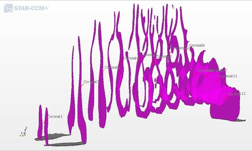
The segmented 3D CAD geometries were imported into the commercial CFD software STAR-CCM+ (v.12.02.011), and these formed the basis for the models. Figure 1 illustrates an imported geometry for geometry 1. The figure also shows the two nostrils as velocity inlet boundary conditions and the nasopharynx as the pressure outlet boundary for the inhalation. At exhalation we investigated the opposite situation, i.e. the nasopharynx became the velocity inlet boundary. In each geometry, twelve coronal cross sections were defined along the nasal passage, see Figure 2 The velocity magnitude in each model corresponds to a physiological flow rate of $Q=166\mathrm{ml}/\mathrm{s}$ (Balakin et al., 2017).

Figure 1. Segmented geometry for case 1.

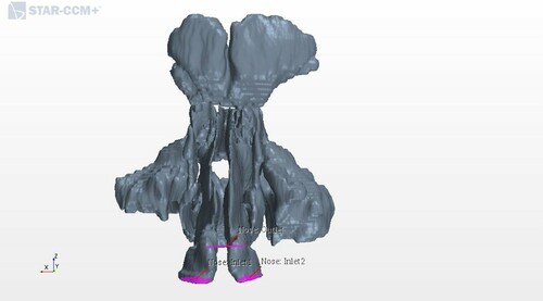
Figure 2. Locations of representative coronal cross sections in the CFD model. The nostrils are on the left and the nasopharynx is on the right.

When simulating the process of inhalation, the inlet velocity was estimated using the frontal area of both the nostrils and the flow rate. The frontal area was computed by the STAR-CCM+ software from the CT images. For the inhalation, the velocities at the inlet for Geometries 1–5 were 1.145 m/s, 0.984 m/s, 0.952 m/s, 1.615 m/s, and 1.020 m/s, respectively. For the exhalation, the velocities at the inlet were 1.293 m/s, 1.082 m/s, 0.900 m/s, 1.068 m/s, and 1.624 m/s, respectively. Because of the low velocities, the flow was assumed to be incompressible due to a low Mach number (less than 0.3). To determine the flow regime, the Reynolds number had to be estimated. The Reynolds number for the nasal airflow was much lower than 2100 in all of the considered cases, so the flow was laminar. The hydraulic diameter of the cross-section was used for the calculation of the Reynolds number.

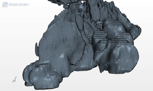
For grid generation, the surface remesher, prism layer mesher, and polyhedral mesher were used in this study. The average size of the polyhedral cells was set to 0.001 m. The size of the prismatic subsurface was 10% of the average and the number of prism layers was equal to two. The size of the grid cells was adjusted to get a satisfactory result; however, smaller cells required a longer computational time. This grid size was tested in the mesh dependence study by Balakin et al. (2017), showing very satisfactory results. Figure 3 shows the applied mesh.

Figure 3. Computational mesh.

This work presents the CFD results for the air flow in the nose during the breathing cycle as well as the particle deposition during inhalation for all five geometries.

A no-slip condition was set at the airway walls, meaning that the air velocity was set to zero at the surface of the nasal membranes lining the nasal cavity. The particles deposited on the wall they collided with, which assumes they were most probably captured by wet mucosa. The density, viscosity, conductivity, and the specific heat of the air were $1.184{\mathrm{kg}/\mathrm{m}}^3$, $1.855\cdot {10}^{-5}\mathrm{Pa}\cdot \mathrm{s}$, $0.026\mathrm{W}/\mathrm{m}\cdot \mathrm{K}$, $1004\mathrm{J}/\mathrm{kg}\cdot \mathrm{K}$, respectively. The particles were assumed to be of spherical shape with a diameter of $50\text{μ}\mathrm{m}$ and a density of $1000{\mathrm{kg}/\mathrm{m}}^3$. It must be noted that this particle diameter does not correspond to particle sizes studied by other researchers, who focused on smaller particles. The initial velocity of the particles was the same as of air. The particles were injected uniformly distributed over the inlet, but they changed their position randomly from one to the next time step to better mimic real conditions. The number flow rate was 10,000 particles per second.

The simulations were carried out using the SIMPLE technique (see e.g. Ferziger & Peric, 2001), realized in the segregated flow solver of STAR-CCM+. The time step was 1 ms. The following under-relaxation factors were selected: pressure 0.3 and velocity 0.7. An average simulation time for one case was 3 hours on 10 cores of 2.6 GHz. The mesh generation was achieved after only 5 min.

3. Results and discussion

In the scientific community there is no agreement about the main mechanism behind the ENS symptoms. Therefore, in this section, we present simulation results for all plausible physiological mechanisms that can cause these symptoms. These include changes in pressure profiles, nasal airway resistance, streamlines and vortex formation, flow partitioning between nostrils, and finally particle deposition during inhalation. For each of the mechanisms, the section highlights the differences between healthy patients and those with ENS and compares the findings to earlier clinical studies. Sufficient differences are observed for all the measured categories.

3.1. Pressure profile

The nasal airway resistance is closely related to the observed distribution of pressures in the nose. The intranasal pressure is the driving force of the breathing function (Balakin et al., 2017). Figures 4 and 5 show the relative pressure distribution for all five geometries during inhalation and exhalation, respectively. The pressure is plotted in the 12 coronal cross-sections. Coronal 1 is nearest to the nostrils, and coronal 12 is at the nasopharynx.

Figure 4. Pressure distribution in the nasal cavity at inhalation. G1, G2, etc. refer to Geometry 1, Geometry 2, etc.

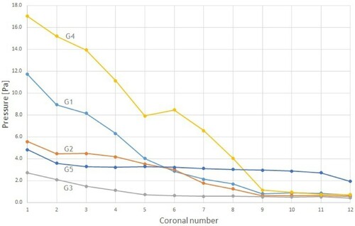
Figure 5. Pressure distribution in the nasal cavity at exhalation. G1, G2, etc. refer to Geometry 1, Geometry 2, etc.

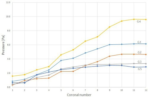
As expected, during inhalation the relative pressure decreased as the distance from the anterior nose increased. However, the two models with ENS showed a rather modest reduction near the nasal valve compared to the cases with obstruction. This was the same as found by Balakin et al. (2017), and can be explained by the difference caused by the partial operational expansion of the channels in the ENS geometries. The obstructed cases are clearly associated with the largest pressure drop within the considered geometries.

During exhalation, the air is expelled from the lungs creating high pressure at the posterior of the nasal cavity. The total pressure drop was similar to inhalation for both the healthy and ENS geometries, see Figure 5. On the other hand, for geometry 1 and 4 with obstructions in the nasal cavity, we observed a pressure drop 38% lower than those at the exhalation phase.

3.2. Nasal airway resistance

Nasal airway resistance is the aerodynamic resistance of the respiratory tract to airflow at inhalation and exhalation. This is an important factor when considering the total nasal airway resistance because nasal breathing is responsible for around 50–80% of all airway resistance. This resistance results from the friction between streaming air and the mucosa (see e.g. Scheithauer, 2011), and is closely related to the inter-nasal pressures described in the previous section. In addition, the resistance plays a vital role in preventing the collapse of the lung (Balakin et al., 2017).

To calculate the resistance R for the studied patients we use the equation from Zhu et al. (2013): (10) $R=\frac{\mathrm{\Delta }P}{Q},$(10) where $\mathrm{\Delta }P$ is the difference in pressure between the nostrils and the nasopharynx, and Q is the volumetric flow rate through the nasal cavity. The calculated values for the studied geometries are shown in Tables 1 and 2.

Table 1. Flow resistance of the models at flow rates of 166 ml/s at inhalation.

Model	Flow resistance $(\frac{\mathrm{Pa}\cdot \mathrm{s}}{\mathrm{ml}})$
Geometry 1: Obstruction	0.06131
Geometry 2: ENS	0.03397
Geometry 3: ENS	0.01728
Geometry 4: Obstruction	0.09682
Geometry 5: Healthy	0.01617

Table 2. Flow resistance of the models at flow rates of 166 ml/s at exhalation.

Model	Flow resistance $(\frac{\mathrm{Pa}\cdot \mathrm{s}}{\mathrm{ml}})$
Geometry 1: Obstruction	0.03037
Geometry 2: ENS	0.02458
Geometry 3: ENS	0.01587
Geometry 4: Obstruction	0.03745
Geometry 5: Healthy	0.03213

The variations in flow resistance are low (except in ENS patients) during exhalation (Table 2). However, during inhalation, we observe a much higher flow resistance for the deviated geometries, which is especially high for the models with obstruction (geometries 1,4), see Table 1. The higher resistance deviated noses are in qualitative agreement with earlier results published by Zhu et al. (2013).

Next, it is important to compare the resistance during exhalation and inhalation. Based on the calculations for the healthy patient, the resistance was higher during exhalation than during inhalation, confirming the observations published in Viani et al. (1990). On the contrary, for deviated geometries (the cases with obstructions and ENS) the residence was lower during exhalation. The most significant difference in resistance was seen in the two models with obstructions. The results correlate to the observed pressure profiles seen in Figures 4 and 5. The significant difference can be attributed to the smaller open area in the nasal cavity of the obstructed geometries compared to the other geometries.

Reduced aerodynamic resistance induced by channel modification might alter nasal aerodynamics and the potential outcome changes microclimate and sensation, thus altering the pulmonary function (Balakin et al., 2017). ENS patients have undergone a surgical enlargement of the internal nasal channels, which is the reason for the very low resistance of geometry 3 in Figure 4. This confirms the findings from Scheithauer (2011) who stated that expansion of the nasal cross-section reduces respiratory resistance.

3.3. Streamlines and vortex formation

Airflow is not only driven by the path of least resistance, but also by its momentum (Keck & Lindemann, 2011; Li et al., 2018). In this section streamlines are used to visualize the flow path inside the nasal cavity, and snapshots for three geometries are presented.

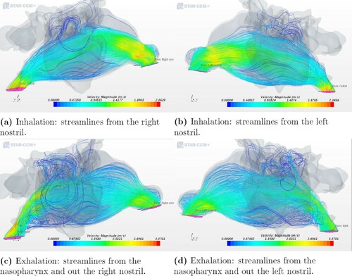
The streamlines differ between inhalation and exhalation. For a majority of patients they are distributed unevenly for the left and right nostrils. To visualize these differences, all figures in this subsection are divided into four subframes: right/left nostrils horizontally and in-/exhalation vertically.

In the case of the healthy patient, see Figure 6, the flow had similar uniform distributions during both inhalation and exhalation, and the streamlines did not show any kind of preferred path. Healthy nasal turbinates play a critical role in conditioning the nasal airflow, which facilitates normal nasal physiology. This includes the capability to warm, humidify, and filter the inhaled airflow while preventing unwanted dehydration of the mucosa (Li et al., 2018).

Figure 6. Airflow patterns for geometry 5 as indicated by streamlines during inhalation and exhalation.

In contrast to the healthy patient, a significant difference in the airflow streamlines pattern was observed in the two ENS geometry models. For geometry 3, the streamlines showed a more uniform distribution of airflow in the nasal cavity at exhalation than at inhalation, which can be seen in Figures 7 and 8. As shown in Figure 7(a,b), the flow goes through the right cavity during the process of inhalation. At exhalation, a more even distribution of airflow pattern was seen, see Figure 7(c,d). The same quantitative pattern was observed at in- and exhalation in the left nasal cavity for the other ENS patient (see Figure 8).

Figure 7. Airflow patterns for geometry 3 as indicated by streamlines during inhalation and exhalation.

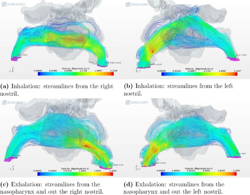
Figure 8. Airflow patterns for geometry 2 as indicated by streamlines during inhalation and exhalation.

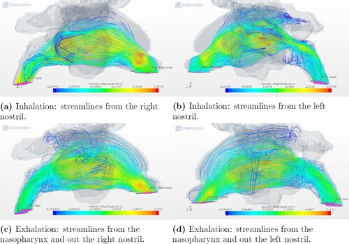
Our results for the ENS patients are in agreement with Li et al. (2018) who also studied the streamlines in the nasal cavity of ENS patients at inhalation. Nasal airflow has a natural tendency to move upwards through the middle meatus region if the proper structures are not in place to distribute the airflow. This is caused by the fact that the airflow must turn 180 ${}^{\circ }$ relative to flow into the lungs in the downward direction, after entering the nostrils in the upward direction. As observed at the posterior part of the nasal cavity during exhalation in both (Li et al., 2018) and this paper, there is a high velocity close to the upper zone of the nasal cavity. This is due to the anatomical features of the nasopharynx that directs the air upwards.

Re-circulatory flow, known as vortices, was prominently observed during exhalation by Riazuddin et al. (2011), and the re-circulatory flow was detected at the lower zone of the posterior region. The vortex-like structures ensure that the air lingers within the nose for a longer period. This results in enhancing the moistening of the inhaled air, as well as the senses of smell and taste that lie above the upper turbinate in the olfactory region (Hörschler et al., 2003).

In the healthy geometry (Figure 6), one can observe vortices for both in- and exhalation. However, for the ENS patients (Figures 7 and 8) there were, for the most part, no well-defined vortices at the anterior part of the nasal cavity or near the olfactory region during inhalation. One reason for this might be the low inlet velocity and the volumetric flow rate. The cause of ENS is a surgery during which the structures in the nose are removed, thus opening the nasal cavity by, for example, severe turbinate reduction. The lack of structures causes abrupt changes in the flow channel and thus fewer vortices. This contributes to a poorer environment in the nasal cavity and may cause the ENS symptoms.

3.4. Flow partitioning

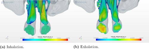
Flow partitioning is defined as the proportion of air flowing through the left and right airways. In this case, the flow partitioning in the nostrils was calculated to see if the flow distribution changed at inhalation and exhalation. The volumetric flow rate Q in the nostrils was calculated based on the frontal area of each nostril and the velocity at the respective inlets. The results of the calculations concerning the flow partitioning in each nostril are presented in percentages and shown in Tables 3 and 4. Also, snapshots of two models showing the velocity distribution in the nostrils are shown in this section.

Table 3. Flow partitioning in the nostrils (%) at inhalation.

	Geometry 1:	Geometry 2:	Geometry 3:	Geometry 4:	Geometry 5:
	Obstruction	ENS	ENS	Obstruction	Healthy
Right (inlet 1)	52.72%	48.83%	50.98%	46.88%	49.71%
Left (inlet 2)	47.27%	51.17%	49.02%	53.12%	50.39%

Table 4. Flow partitioning in the nostrils (%) at exhalation.

	Geometry 1:	Geometry 2:	Geometry 3:	Geometry 4:	Geometry 5:
	Obstruction	ENS	ENS	Obstruction	Healthy
Right (outlet 1)	26.56%	59.69%	48.15%	22.36%	51.88%
Left (outlet 2)	73.55%	40.31%	51.85%	77.64%	48.12%

In all five models, the simulation provides different flow partitioning for in- and exhalation. The greatest difference is seen at exhalation and in the two geometries with an obstruction in the nasal cavity. The flow partitioning for geometry 1 shifted between the two nostrils from 52.72% on the right and 47.27% on the left during inhalation to 26.56% on the right and 73.55% on the left during exhalation. The same significant difference was seen for geometry 4. It corresponds to a considerably higher flow resistance in the right nasal cavity in both models at inhalation (see Figure 4). This can be explained by the low cross-sectional area in the right nasal cavity, which prevents the air from flowing easily through it during exhalation.

It is of interest to compare our results with previously published observations. Hildebrandt et al. (2013) analyzed the overall flow partitioning between two nasal cavities, one from a healthy case and the other from a symptomatic case. The flow partitioning in the two nasal cavities shifted from 56% on the right and 44% on the left to 53% on the right and 47% on the left. This was due to a decline in the flow space constriction in the anterior part of the left nasal cavity, which was a result of a repaired deviated septum. We observed a similar shift between geometries 1 and 2, corresponding to the pre- and post-operation conditions of a patient. The result shows a shift in the flow partitioning rate distribution at exhalation from 26.56% on the right and 73.55% on the left for geometry 1 to 59.69% on the right and 40.31% on the left for geometry 2. A visualization of the velocity distribution is illustrated in Figures 9 and 10, where the nostril with the highest velocity is also the one with the highest flow partitioning percentage out of the two nostrils.

Figure 9. Velocity distribution in the nostrils for geometry 1.

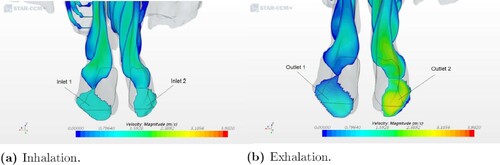
Figure 10. Velocity distribution in the nostrils for geometry 2.

3.5. Particle deposition

The particles that deposit in the nasal cavity during inhalation do not reach the lungs, and thus the nose acts as a barrier for the lung deposition. In addition, nasal deposition is important in relation to the estimation of toxic doses from inhaled aerosols (Lippmann, 1970). To quantify the deposition of particles, it is common to define deposition efficiency as the ratio of the number of particles deposited to the number of particles injected.

In this research, the simulations were conducted to see if the different intranasal structures and conditions had any influence on the number of particles deposited. The deposition efficiency can be computed by post-processing the CFD simulations. Table 5 summarizes the efficiency for each of five geometries. For most geometries including the healthy patient, the deposition efficiency stays around $0.5\pm 0.1$.

Table 5. Particle deposition in the nasal cavity.

Model	Number of particles injected	Number of particles deposited	Deposition efficiency
Geometry 1: Obstruction	99	51	0.5152
Geometry 2: ENS	89	37	0.4157
Geometry 3: ENS	100	18	0.1800
Geometry 4: Obstruction	95	55	0.5789
Geometry 5: Healthy	96	38	0.3958

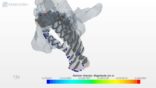
The only exception is the deposition efficiency for geometry 3, corresponding to one of the ENS patients, see Figure 11. The value obtained of 0.18, which is less than 50% from the second smallest result in the study can be attributed to changes caused by a nasal surgery. After a surgery, the patients had a wider passage of the nasal cavity, and this caused the bulk of inhaled air to have little contact with the remaining mucosal wall. Sozansky and Houser (2015) state that with a reduced mucosal surface area for the air to interact with, and a lack of physiological turbulent airflow seen in ENS patients, the nasal mucosa cannot carry out its primary functions of air conditioning and cleaning of particles. This could be connected to what was discussed in Section 3.3 where the airflow in the ENS and obstruction geometries did not have the same uniform velocity distribution as in the healthy patient. The slower airflow of an ENS geometry would seem to be beneficial because it increases the time that the air is in contact with mucosa. However, the laminar quality of the slow airflow in ENS patients prevents extensive interaction of flowing air particles with the nasal mucosa, which is in accordance with Sozansky and Houser (2015).

Figure 11. Lateral view of the particles deposited in the nasal cavity for geometry 3.

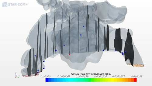
On the other side of the spectrum is deposition for obstructed geometry 4. In Figure 12 on can see a large number of particles in the nasal cavity, and this is most likely due to the obstruction on the right side where the particles deposit. Cheng et al. (1996) pointed out that a smaller cross-sectional area indicates a higher nasal deposition, which corresponds to the results shown in Table 5.

Figure 12. Snapshot taken from above of the particles deposited in the nasal cavity for geometry 4.

Finally, it is of interest to compare geometry 1 and 2 to see how the operational removal of an obstruction influences particle deposition. During septoplasty or turbinate reduction surgery, the nasal mucosa are normally reduced, thus reducing the area to which particles can stick. Expectedly, geometry 2 shows a lower deposition efficiency compared to the pre-operative model of geometry 1. The reduced depositional efficiency might be among the causes of sensitive changes result in the ENS syndrome.

4. Conclusion

This study aims at studying flow patterns in the nasal cavity and comparing nasal aerodynamics during inhalation and exhalation. Here we consider geometries acquired by means of CT data from four individuals, including two who had developed ENS.

Based on the results of this study, the influence of geometrical variations in the nasal cavity due to obstruction or surgery was found to produce quite significant differences in the physical parameters. The increase of pressure and flow resistance was observed because of the blockage on one side in the nasal cavity for obstructed geometries 1 and 4. Contrarily, geometry 3 with ENS showed very low resistance values of $0.01728\mathrm{Pa}\cdot \mathrm{s}/\mathrm{ml}$ at inhalation and $0.01587\mathrm{Pa}\cdot \mathrm{s}/\mathrm{ml}$ at exhalation compared to the other models, most likely due to the surgical enlargement that ENS patients have undergone. Furthermore, the overall resistance value was lower at the exhalation phase compared to the inhalation phase for all the models except for the healthy patient.

The observed streamlines in the nasal cavity were distributed more uniformly at exhalation than at inhalation for all of the models. Furthermore, vortices were observed in the posterior region of the models at exhalation. Flow partitioning in the nostrils showed a change from that nostril that had the highest volumetric flow rate from inhalation to exhalation, and the most significant difference was seen in the two obstruction models.

ENS geometry 3 showed a particle deposition ratio of 0.18 that was much lower than for the other patients. Also, post-operative geometry 2 (with ENS) had a lower particle deposition ratio than pre-operative geometry 1 corresponding to the same patient. This was despite a greater patency in the nasal cavity. In this case, the deposition ratio went down from 0.5152 to 0.4157. This might be due to the reduced mucosal area, which is common for ENS patients. However, to determine if the reduced mucosa influences the low deposition ratio, it would be preferable for future work to use a larger sample of both ENS patients and healthy controls. There is also a need to perform experimental work on fluid flow structure in the nasal cavities, either in-vivo or in artificial geometries that correspond to patients' anatomy.

Acknowledgements

This study was supported by the Research Council of Norway (project 300286).

Disclosure statement

No potential conflict of interest was reported by the author(s).

Additional information

Funding

This work was supported by Norges Forskningsråd [grant number 300286].

References

- Akbarian, E., Najafi, B., Jafari, M., Ardabili, S. F., Shamshirband, S., & Chau, K. W. (2018). Experimental and computational fluid dynamics-based numerical simulation of using natural gas in a dual-fueled diesel engine. Engineering Applications of Computational Fluid Mechanics, 13, 517–534. https://doi.org/https://doi.org/10.1080/19942060.2018.1472670
- Balakin, B. V., Farbu, E., & Kosinski, P. (2017). Aerodynamic evaluation of the empty nose syndrome by means of computational fluid dynamics. Computer Methods in Biomechanics and Biomedical Engineering, 20, 1554–1561. https://doi.org/https://doi.org/10.1080/10255842.2017.1385779
- Brüning, J., Hildebrandt, T., Heppt, W., Schmidt, N., Lamecker, H., Szengel, A., Amiridze, N., Ramm, H., Bindernagel, M., Zachow, S., & Goubergrits, L. (2020). Characterization of the airflow within an average geometry of the healthy human nasal cavity. Scientific Reports, 10(1), 3755. https://doi.org/https://doi.org/10.1038/s41598-020-60755-3
- Cheng, Y. S., Yeh, H. C., Guilmette, R. A., Simpson, S. Q., Cheng, K. H., & D. L. Swift (1996). Nasal deposition of ultrafine particles in human volunteers and its relationship to airway geometry. Aerosol Science and Technology, 25, 274–291. https://doi.org/https://doi.org/10.1080/02786829608965396
- Crowe, C. T., Schwartzkopf, J. D., Sommerfeld, M., & Tsuji, Y. (2012). Multiphase flows with droplets and particles. CRC Press.
- Di, M. Y., Jiang, Z., Gao, Z. Q., Li, Z., An, Y. R., & Lv, W. (2013). Numerical simulation of airflow fields in two typical nasal structures of empty nose syndrome: A computational fluid dynamics study. PLOS ONE, 8(12 https://doi.org/https://doi.org/10.1371/journal.pone.0084243
- Ferziger, J. H., & Peric, M. (2001). Computational methods for fluid dynamics. Springer-Verlag.
- Garcia, G. J., Tewksbury, E. W., Wong, B. A., & Kimbell, J. S. (2009). Interindividual variability in nasal filtration as a function of nasal cavity geometry. Journal of Aerosol Medicine and Pulmonary Drug Delivery, 22(2), 139–155. https://doi.org/https://doi.org/10.1089/jamp.2008.0713
- Ghalandari, M., Koohshahi, E. M., Mohamadian, F., Shamshirband, S., & Chau, K. W. (2019). Numerical simulation of nanofluid flow inside a root canal. Engineering Applications of Computational Fluid Mechanics, 13, 254–264. https://doi.org/https://doi.org/10.1080/19942060.2019.1578696
- Hildebrandt, T., Goubergrits, L., Heppt, W., Bessler, S., & Zachow, S. (2013). Evaluation of the intranasal flow field through computational fluid dynamics. Facial Plastic Surgery, 29(2), 93–98. https://doi.org/https://doi.org/10.1055/s-00000018
- Hörschler, I., Meinke, M., & Schröder, W. (2003). Numerical simulation of the flow field in a model of the nasal cavity. Computers & Fluids, 32(1), 39–45. https://doi.org/https://doi.org/10.1016/S0045-7930(01)00097-4
- Inthavong, K., Fung, M. C., Yang, W., & Tu, J. (2015). Measurements of droplet size distribution and analysis of nasal spray atomization from different actuation pressure. Journal of Aerosol Medicine and Pulmonary Drug Delivery, 28(1), 59–67. https://doi.org/https://doi.org/10.1089/jamp.2013.1093
- Inthavong, K., Wen, J., Tu, J., & Tian, Z. (2009). From ct scans to cfd modeling – fluid and heat transfer in a realistic human nasal cavity. Engineering Applications of Computational Fluid Mechanics, 3(3), 321–335. https://doi.org/https://doi.org/10.1080/19942060.2009.11015274
- Issakhov, A., Bulgakov, R., & Zhandaulet, Y. (2019). Numerical simulation of the dynamics of particle motion with different sizes. Engineering Applications of Computational Fluid Mechanics, 13, 1–25. https://doi.org/https://doi.org/10.1080/19942060.2018.1545253
- Keck, T., & Lindemann, J. (2011). Numerical simulation and nasal air-conditioning. GMS Current Topics in Otorhinolaryngology, Head and Neck Surgery, 9. https://doi.org/https://doi.org/10.3205/cto000072
- Li, C., Farag, A. A., Leach, J., Deshpande, B., Jacobowitz, A., Kim, K., Otto, B. A., & Zhao, K. (2017). Computational fluid dynamics and trigeminal sensory examinations of empty nose syndrome patients. The Laryngoscope, 127, E176–E184. https://doi.org/https://doi.org/10.1002/lary.26530
- Li, C., Farag, A. A., Maza, G., McGhee, S., Ciccone, M. A., Deshpande, B., Pribitkin, E. A., Otto, B. A., & Zhao, K. (2018). Investigation of the abnormal nasal aerodynamics and trigeminal functions among empty nose syndrome patients. International Forum of Allergy & Rhinology, 8, 444–452. https://doi.org/https://doi.org/10.1002/alr.22045
- Lippmann, M. (1970). Deposition and clearance of inhaled particles in the human nose. Annals of Otology, Rhinology & Laryngology, 79, 519–528. https://doi.org/https://doi.org/10.1177/000348947007900314
- Ramezanizadeh, M., Nazari, M. A., Ahmadi, M. H., & Chau, K. W. (2019). Experimental and numerical analysis of a nanofluidic thermosyphon heat exchanger. Engineering Applications of Computational Fluid Mechanics, 13, 40–47. https://doi.org/https://doi.org/10.1080/19942060.2018.1518272
- Riazuddin, V. N., Zubair, M., Abdullah, M. Z., Ismail, R., Shuaib, I. L., Hamid, S. A., & Ahmad, K. A. (2011). Numerical study of inspiratory and expiratory flow in a human nasal cavity. Journal of Medical and Biological Engineering, 31, 201–206. https://doi.org/https://doi.org/10.5405/jmbe.781
- Scheithauer, M. O. (2011). Surgery of the turbinates and empty nose syndrome. GMS Current Topics in Otorhinolaryngology, Head and Neck Surgery, 9, 1–28. https://doi.org/https://doi.org/10.3205/cto000067
- Sozansky, J., & Houser, S. M. (2015). Pathophysiology of empty nose syndrome: Pathophysiology of empty nose syndrome. The Laryngoscope, 125, 70–74. https://doi.org/https://doi.org/10.1002/lary.24813
- Tu, J., Inthavong, K., & Ahmadi, G. (2012). Computational fluid and particle dynamics in the human respiratory system. Springer Science & Business Media.
- Viani, L., Jones, A. S., & Clarke, R. (1990). Nasal airflow in inspiration and expiration. The Journal of Laryngology & Otology, 104, 473–476. https://doi.org/https://doi.org/10.1017/S0022215100112915
- Wexler, E., Segal, R., & Kimbell, J. (2005). Aerodynamic effects of inferior turbinate reduction: Computational fluid dynamics simulation. Archives of Otolaryngology Head & Neck Surgery, 131, 1102–1107. https://doi.org/https://doi.org/10.1001/archotol.131.12.1102
- Zhu, J. H., Lee, H. P., Lim, K. M., Lee, S. J., Teo Li San, L., & Wang, D. Y. (2013). Inspirational airflow patterns in deviated noses: A numerical study. Computer Methods in Biomechanics and Biomedical Engineering, 16, 1298–1306. https://doi.org/https://doi.org/10.1080/10255842.2012.670850