Clocking effect of outlet RGVs on hydrodynamic characteristics in a centrifugal pump with an inlet inducer by CFD method

Abstract

This paper investigates the hydrodynamic characteristic of a single-stage centrifugal pump with inlet inducer and outlet Radial Guided Vanes (RGVs) influenced by the clocking effect for the first time. Different from general ones, the outlet RGVs in this paper have specificities. The hydraulic performance and dynamic characteristics of the centrifugal pump are numerically studied and validated by experiments. The results indicate that there is an optimum position of RGVs that can not only increase the pump head and efficiency but also reduce the pressure fluctuation intensity. A non-dimensional parameter describing the velocity non-uniformity of the impeller outlet is first proposed, which is negatively related to the pump’s hydraulic performance. The clocking position of the RGVs will affect the velocity homogeneity at the impeller outlet, and further influence the hydraulic characteristics of the pump. Besides, the clocking effect of outlet RGVs mainly affects the amplitudes of BPF for both the pressure fluctuation and radial force, and the most obvious frequency of pressure pulsation and radial force is 3 BPF correlating with the inlet inducer. It is recommended to install the volute-tongue tip near the middle of two vanes.

KEYWORDS:

• Clocking effect
• centrifugal pump
• radial guide vane
• inlet inducer
• pressure fluctuation
• hydraulic performance

1. Introduction

The guide vanes, having the effect of reducing the radial thrust by adjusting the internal flow direction, are widely adopted in pumps, turbines, and compressors, especially at high-pressure conditions. The hydrodynamics of the pump will be influenced by changing the relative position between the Radial Guide Vanes (RGVs) and the volute tongue in the circumferential direction, which is referred to as the clocking effect. If improperly designed, the clocking effect will result in high-pressure fluctuations, structure vibration, and even piping rupture in the pump system. However, the designers often neglect the location of the RGVs in the practical design and installation process of pumps (Tan, He, Liu, Dong et al., 2016).

Originally, the clocking effect is a phenomenon rising in compressors and turbines when either the rotors generate different phases or the stators are installed at different circumferential positions. As early as 1972, Walker and Oliver (1972) and his colleagues.studied the clocking effect in an axial flow compressor. They found that the noise generated by blade interaction could be effectively reduced by properly adjusting the circumferential position of the rotor in a compressor. Later on, the clocking effect is proved to greatly affect the performances and unsteady aerodynamic dynamics, and many investigators tried to find the optimal clocking position to maximize the efficiency and get the best transient behaviors (Behr et al., 2006; Dieter et al., 2005; Haldeman et al., 2005; Saren et al., 1998). In recent years, some researchers are focusing on the clocking effect in more areas. Staeding et al. (2012) confirmed that stator clocking weakened the advantages of air-foil indexing overall in an axial compressor. Smith and Key (2013) investigated the clocking effect on stall margin and found that vane clocking without impacting stall margin was a good way to improve the performance in a multistage compressor. Key (2014) indicated that the impact of the upstream-vane wake led to the best performance at the design point but the lowest efficiency at off-design conditions for compressors.

Pumps, like compressors and turbines, pertaining to the frame of rotating machinery, are also affected by the clocking effect. There are four categories of clocking positions in pumps: inlet guide vanes with volute, outlet guide vanes with volute, inlet guided vane with impeller, and impeller with impeller in multistage pumps. In recent years, some studies have focused on the clocking effect in the pumps. Qu et al. (2016) and Deng et al. (2016) numerically studied the clocking effect on the flow field and pressure pulsation in centrifugal pumps with inlet guide vanes. The same work was carried out on pumps with the outlet guide vanes by Liu et al. (2013), Jiang et al. (2016), and experimentally validated by Wang et al. (2018). Tan, He, Liu, Wu, et al. (2016) tested the clocking effect of impellers in a five-stage pump and found the clocking positions of impellers had little impact on the pump’s head and efficiency but greatly influenced the structure vibration.

The above literature has revealed some basic facts that the clocking effect is non-negligible in pumps with either inlet inducer or outlet guide vanes. Scholars are paying an increasing attention to find the optimal circumferential position of guide vanes, concerning enhancing the performance and diminishing the flow regime pulsation at the same time. Some suggestions are given but non-uniform for different pumps. Wang et al. (2018) suggested the outlet diffuser should near the volute tongue with much lower pulsation and almost unchanged performance after the testing investigation of three positions. The research of Jiang et al. (2016) proposed that the volute tip should be near the middle of two vanes to get better performance and lower radial forces.

With the development of computational fluid dynamics (CFD) techniques, numerical simulation has become a powerful and reliable tool for analysis in turbomachinery. In 2013, Shah et al. (2013) had a systematic review of CFD application for centrifugal pumps in performance prediction, parametric study, cavitation analysis, and fluid-structure interaction. Pinto et al. (2017) provided a more comprehensive overview of the latest application of CFD in turbomachinery, including compressors, turbines, and pumps. More and more researchers regard CFD as an indispensable tool to investigate extended topics, such as the flow-induce noises in pumps (Si et al., 2019) and multi-objective optimization of impeller blades in the mixed flow pump (Dash et al., 2018; Suh et al., 2019). More uses are extended to other fields. Chao et al. (2019) studied the effect of inclined cylinder ports on gaseous cavitation in a high-speed electro-hydrostatic actuator pump. Ramezanizadeh et al. (2019) computed the performance of a thermosyphon-based heat exchanger of the latest design with a new approach based on CFD. Munih et al. (2020) developed a CFD-based procedure to allow studying flow and pressure conditions in a tumbling multi-chamber gear pump. Abadi et al. (2020) adopted CFD to evaluate the affecting variables on the energy efficiency of a novel regenerative evaporative cooler. In a word, an increasing number of researchers are considering CFD as a reliable, feasible, and accurate way in many fields, including the dynamics of turbo-machinery.

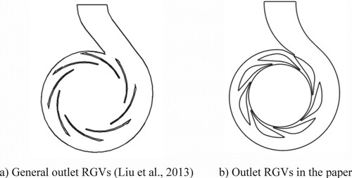
In the paper, the clocking effect of the outlet RGVs is studied in a single-stage centrifugal pump with both the inlet inducer and outlet RGVs by CFD tools. The performance and unsteady flow pulsations of the pump are analysed. Different from general outlet diffusers (Jiang et al., 2016; Liu et al., 2013) whose cross-section area of the blade basically remains unchanged in the radial direction, the blade of the outlet RGVs in the paper is very special. The cross-section area of the outlet guide vane increases greatly along the radial direction and the suction side of the vane is of high curvature as shown in Figure 1. An attempt is made to explain the essential reasons for the clocking effect on the pump hydraulic characteristics.

Figure 1. Comparison of outlet RGVs.

2. Numerical simulation procedures

2.1. Pump parameters and computational domain

The pump model is a single-stage industrial centrifugal pump, which consists of four units: (a) an inducer with 3 inlet guide vanes to improve the flow pattern into the impeller; (b) an impeller composed of 5 backward blades and 5 additional splitter blades; (c) a diffuser with 7 radial guide vanes to collect the liquid from the impeller and smoothly guide it into the volute; (d) a volute. Moreover, pipes are extended at the inlet and outlet of the domain to ensure full development of the flow. The overview of the 3-D pump model is illustrated in Figure 2, and more detailed parameters are listed in Table 1. Furthermore, a spatial Cartesian coordinate system is established as shown in Figure 2, the origin of the coordinate is located in the axial of the pump, and the Z direction is determined by the right-hand rule.

Figure 2. Overview of the 3-D pump model.

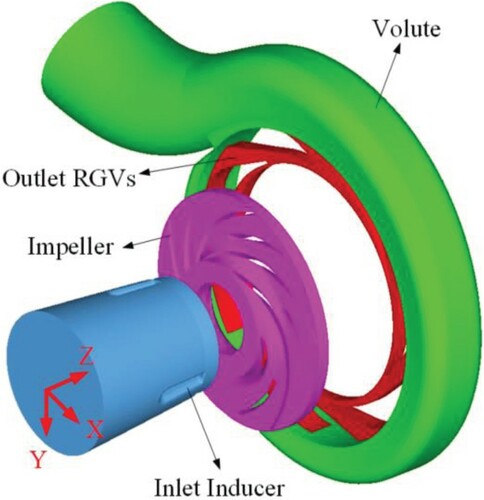
Table 1. Main parameters of the centrifugal pump.

Item	Value
Design flow rate Qr (m^3/h)	59.3
Rotational speed ω (rad/s)	100 π/s (i.e.3000 rpm)
Rotational frequency (fn)	50 Hz
Pump design head (m)	78
Design specific speed Ns	14.7
Impeller exit width b (m)	0.011
Impeller exit diameter d (m)	0.240
Blade numbers of impeller	5 long, 5 short
Inlet guide vane numbers of inducer	3
Radial guide vane numbers of diffuser	7
Diameter of inlet (m)	0.15
Diameter of outlet (m)	0.125
Pre-whirl angle of inlet guide vane (°)	0
Angle between two sequential impeller blades (°)	51.43

To investigate the clocking effect, five clocking positions are set (named CL0, CL1, CL2, CL3, and CL4, respectively), by changing the relative angle between the RGVs and the volute tongue tip along the circumferential direction with an average interval of 10^o (as shown in Figure 3).

Figure 3. Schematic diagram of the 5 clocking positions.

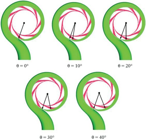
It should be pointed out that CL0 is the actual installation angle of the RGVs of the pump in test. Besides, the inlet inducer is fixed.

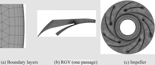
Considering the complexity of the pump, the unstructured grids are adopted. The tetrahedral grids exist in the majority area and the pentahedral prism grids are generated for the boundary layer. The boundary layer is refined considering flow separation and pressure gradients. Away from the solid wall, the grid is stretched, which can effectively reduce the gird number and the calculation cost based on the accuracy and the reliability of computation. The meshes around the blade edges, volute tongue, and RGVs are locally refined as shown in Figure 4.

Figure 4. Mesh of the pump in different domains.

As is known, the variable y⁺ is a wall distance value to assure the thickness of the grid boundary layer in a reasonable range corresponding to the turbulence model. The definition of y⁺ is as follows: (1) $\begin{array}{rl}{y}^{+}& =(y\cdot u_{\tau })/\nu \end{array}$(1) (2) $\begin{array}{rl}{u}_{\tau }& =\sqrt{{\tau }_w/\rho }\end{array}$(2) where y is the vertical height of the first boundary layer to the wall, and ν, τ_w, and ρ are the kinematic viscosity, shear stress, and fluid density, respectively. The value of y⁺ will be given below.

2.2. Turbulence model

SST k-ω model is adopted to provide turbulence closure for its advantage in simulating the internal flow of pumps (Shuai et al., 2014). The k-ω formulation in the SST k-ω model is effective in dealing with the low-Reynolds-number turbulence in the boundary layers all the way down to the structure without any extra damping functions (Menter, 1994), as the flow conditions of the boundary layers near the wall are of low-velocity and viscous. In the simulation of the free stream, the SST k-ω formulation also performs well as it can take the advantages of the k-ϵ formula to avoid the common k-ω problem that it is greatly affected by the inlet turbulence properties.

2.3. Numerical method and conditions

The commercial CFD code, ANSYS CFX is used to solve the continuity and momentum equations of the flow inside the pump. The finite volume method is adopted to discretize the three-dimensional governing equations. A total pressure boundary condition is specified at the inlet. The outlet boundary is set as the mass flow rate condition. The no-slip condition is imposed on the walls. Due to the impeller rotation, two different computation regions are formed: the rotating domain of impeller and other stationary domains (i.e. inducer, RGVs, and volute). The two kinds of domains are interrelated by imposing two interfaces at the inlet and outlet of the impeller with their adjacent domains. Due to different grids between two contact interfaces, the mesh connection is set to the general grid interface (GGI). In steady calculations, an angular position of the impeller is fixed and the interaction between the moving part and the still parts is accomplished utilizing Frozen Rotor Method.

The numerical simulation starts with a steady flow calculation, and the pump hydraulic performances at different clocking positions are obtained. Once the convergence of the steady simulation is realized, the pressure and velocity fields are used as the pre-conditions to initialize unsteady flow calculations.

The Sliding Mesh technique is utilized to simulate the rotor-stator interaction in unsteady simulations, which will show the circumferential position variation between the rotating impeller and its adjacent stationary parts. The interfaces at the inlet and outlet of the impeller are set as rotor-stator interfaces, while the others between the stationary components are set as the general grid interface. The second-order implicit format is adopted to discretize the time domain and SIMPLE-C algorithm for the coupling of velocity and pressure. The frame change/mixing model is set as the transient rotor-stator. The turbulence intensity is initially set to 5%. The convergence criterion is set to 1×10⁻⁴, allowing an optimal number of iterations for each time step.

Two non-dimensional parameters, flow coefficient Φ, and head coefficient Ψ, are introduced (Barrio et al., 2011). They are defined as follows: (3) $\begin{array}{rl}\mathrm{\Phi }& =Q/(\omega d^{2}b)\end{array}$(3) (4) $\begin{array}{rl}\mathrm{\Psi }& =gH/({\omega }^2{d}^2)\end{array}$(4)

After the governing equations and numerical method approaches are determined, grid-independence analysis is conducted at the design flow rate, as shown in Figure 5.

Figure 5. Mesh grids independence analysis.

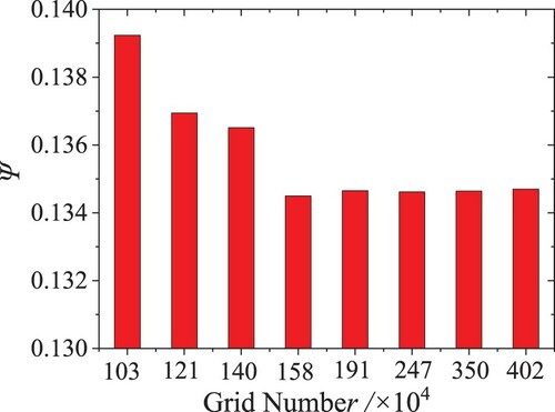
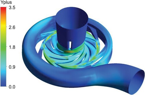
When the total grids number reaches 1.58 × 10⁶, the pump head nearly remains unchanged. However, in order to capture the flow regime of the pump more accurately, the mesh system with 4.02 × 10⁶ cells is employed. In this case, the value of y+ is close to 1 in most regions and the maximum value is 3.5 near the end of inlet vanes as shown in Figure 6, which is reasonable for the turbulence computation of the SST k-ω model.

Figure 6. y Plus contour of the computational domain.

2.4. Experiments validation

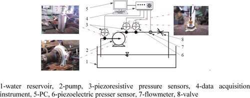
In order to verify the reliability of simulations, experiments about the hydraulic performance of the pump are conducted in an open test system (seeing Figure 7). Two fast-response piezoresistive pressure sensors (CYG-401, SQ) are mounted at the inlet and outlet of the pump to record the static pressure signals with a high sample frequency of 20 kHz and uncertainty of 0.2%. A piezoelectric pressure sensor (106B51-PCB), with the resolution of 0.1% FS and uncertainty of 0.1%, is fixed at the outlet pipe to obtain the local pressure pulsation. The flow rates are measured by a turbine flowmeter (LDG-32S, XE) mounted on the outlet pipe, with a maximum deviation of $\pm$1.5% when working at the low-flow-rate conditions. All signals are collected and stored by the acquisition instrument (3560C-B&K).

Figure 7. Layout of the experimental test system.

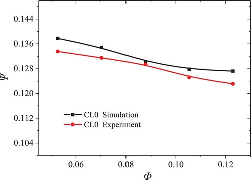
Due to the practical limitations, only the confirmatory tests for Case CL0 are conducted, and the simulated and experimental results of the pump heads are compared in Figure 8. The simulated heads consist well with the experiment data at different flow rates. The relative difference between the experimental and the numerical data remains below 3% for all the tested flow rates for Case CL0. It proves the accuracy and reliability of the calculation procedure on the prediction of the pump’s hydraulic performance. Therefore, we believe that the simulating results of the other four cases with the same method are of good credibility.

Figure 8. Pump head obtained numerically and experimentally at Case CL0.

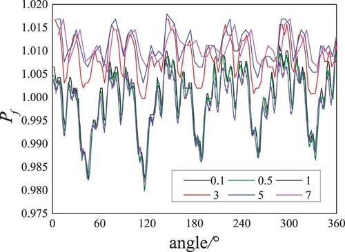
In unsteady analysis, time-step independence analysis is carried out by computing Case CL0 at the design flow rate. The basic unit of the time step is 5.556 × 10⁻⁵ s, corresponding to the impeller passing 1^o. Six time steps are computed, changing from 0.1 basic units to 7 basic units as shown in Figure 9. P_f is a non-dimensional coefficient, which is the ratio of the outlet pressure at each time step to a constant pressure. The constant pressure is the mean value of the outlet pressure in one circle. It shows that outlet pressure calculated by different time steps varies quite little when the time step is smaller than 1 basic unit. Therefore, the time step is 1 basic unit, namely 5.556 × 10⁻⁵ s in the following context.

Figure 9. Time-step independence analysis for the unsteady calculation.

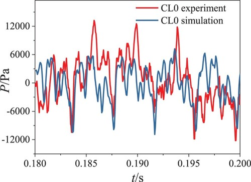
After the pump running stable, a section of pressure signals is extracted to do the comparative analysis, as seen in Figure 10, which shows the pressure pulsation at the pump outlet over one period of time for Case CL0. It can be seen that rotor-stator interaction is obvious as there are five troughs in one cycle. There are three bumps between two adjacent troughs in both experimental and simulated curves corresponding to three vanes of inducer. Moreover, the values of the experiment and the simulation at every trough are nearly the same in one period.

Figure 10. Pressure fluctuations in the time domain at Q_r of Case CL0.

From the frequency diagram in Figure 11, the obvious frequencies are labeled. It can be seen that the main frequencies for both simulation and experiment are the blade passing frequency (BPF) and its third harmonics concerning the inducer with three vanes. Because of the rotor-stator interaction, the seventh orders of the rotating frequency and BPF are of high amplitude for the RGVs with seven vanes.

Figure 11. Power spectrum density of pressure fluctuation at the outlet in the frequency domain at Q_r of Case CL0.

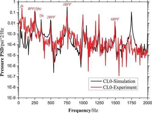
As for the discrepancies of amplitudes and frequencies between experimental and numerical results, it is obvious that the experimental curves have some new characteristic frequencies, such as fn with a high amplitude and 2 fn. Besides, experimental amplitudes are generally larger than numerical ones at the hydraulic-relating frequencies. The reasons are as follows. The pump is driven by an electric motor, a rigid shaft coupling connects the motor and the pump. The pump shaft, motor shaft, coupling, and support bearings comprise a complex rotor system. Inevitably, there are parallel misalignment and angular misalignment in the rotor system, which will result in the characteristic frequencies of fn and 2 fn. The coupling effect between the rotor system and the fluid amplifies the unsteadiness of the fluid fields to some extent. The mechanism will lead to new coupling frequencies and higher amplitudes in comparison with the simulation process, which computes the flow field at a constant rotating speed. Otherwise, the differences may be caused by an installation error, surroundings, and the like, which are not emphasized in the paper. So there are discrepancies between the numerical and experimental results because the simulation could not take all the practical influencing factors into consideration. However, the comparison results already show a good agreement for most hydraulic-relating frequencies.

As a whole, there is a general good agreement between the experiments and the simulations at the clocking angle 0^o (CL0). The comparison results somehow verify the accuracy of the transient computation procedure.

3. Results and discussion

3.1. Steady analysis

The steady calculation analyse the hydraulic performance of the pump: the pump head, efficiency at each position in this section, and finally a non-dimensional coefficient is proposed.

3.1.1. Hydraulic performance

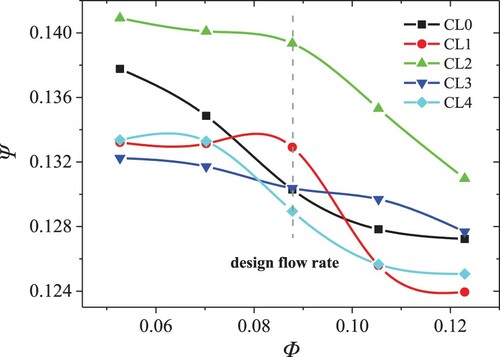
The Influence of the clocking positions on the pump head is shown in Figure 12. There are several distinct features.

1. At a fixed clocking position, the pump heads generally decline with the increment of the mass flow rate for all curves.

2. Apparently, at clocking position CL2, the pump head is obviously higher than the other four conditions at all flow rates.

3. At the lower-flow-rate conditions, the pump head of CL1 remains almost unchanged while once above the design point (it seems like a threshold), the pressure head decreases rapidly with the flow increasing.

4. The slope of the curve CL3 is most moderate among the five situations, while the curve CL0 is steepest at lower flow rates.

Figure 12. Influence of clocking positions on the pump head.

In a word, the five curves show great diversity and randomness due to the location variation of RGVs. The relationship of the pressure head and flow rate at one certain clocking angle cannot be extrapolated to the other angles; therefore, it is hard to establish a fixed formula to elucidate the interrelation between pump head and clocking angle accurately.

For quantitative comparison, a non-dimensional parameter head difference (HD) is defined: HD = (Ψ_CLi – Ψ_CL0) / Ψ_CL0 × 100%, where Ψ_CL0 is pump head for Case CL0 as a reference, and Ψ_CLi is pump head for Cases CL1, CL2, CL3, and CL4. At design condition, the maximum HD is 6.9% between position CL2 and CL0; For Cases CL1, CL3 and CL4, the HDs are 2.0%, 0.1%, −1.0%, respectively. It shows that under the design condition, the head increases first and then decreases as the angle increases gradually. Therefore, there is an optimal angle between RGVs and the volute to improve the pump head.

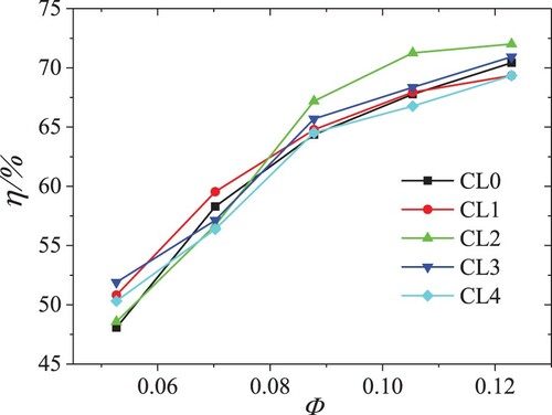
Figure 13 illustrates the variation tendency of the hydraulic efficiency vs. mass flow rate at five different clocking positions. It is clear that Case CL2 has the highest hydraulic efficiency than other cases at larger flow rates. In contrast, hydraulic efficiency is relatively lower at position CL4 nearly at all flow rates. A non-dimensional parameter efficiency difference (ηD): ηD = (η_CLi – η_CL0) / η_CL0 × 100% is defined, where hydraulic efficiency η_CL0 for Case CL0 is used as a reference, and η_CLi is hydraulic efficiencies for the Cases CL1, CL2, CL3, and CL4. At the design flow rate, the maximum ηD is 4.4% between position CL2 and CL0, versus 0.6%, 2.0%, and 0.2% for the other 3 cases. In summary, the clocking position of CL2 (20^o) can best improve pump efficiency.

Figure 13. Influence of clocking positions on pump efficiency.

Therefore, in comparison with the other four cases, it can be seen that when the clocking angle between the guide vanes and volute is 20^o (CL2), the pump head and efficiency can be maximized at the design rate condition. Comprehensively speaking, Case CL2 has the best hydraulic performance.

3.1.2. Internal velocity field

The velocity fields inside the pump at the design flow rate of 5 clocking positions are shown in Figure 14. It is found that the velocity distribution is highly inhomogeneous in the diffuser domain and the flow regime in the diffuser is counter-clockwise. Taking a closer look at the velocity contours, some of the fluid with higher speed that passes through the guide vanes forms ‘velocity wake bands’ in the volute. Such as Case CL0, the ‘velocity wake bands’ are obvious on the left side of the volute tongue and at the upper zones of the volute as shown in Figure 14. Additionally, the ‘bands’ distribute differently in the circumferential direction in each case due to different clocking positions.

Figure 14. Velocity contours in impeller and volute domain.

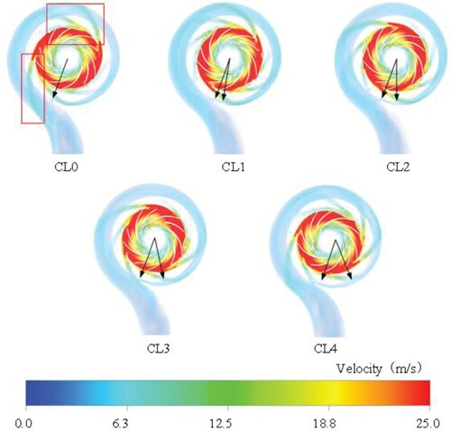
If the ‘velocity wake band’ has a large radial component, the flow out of the RGVs will impact the volute wall, which will lead to hydraulic loss. For example, in Case CL4, the velocity wakes will thrust the wall at the regions marked by the letter A and B, as specified in Figure 15. It also demonstrates that the velocity fields are not uniform in the circumferential direction, either in the impeller or in RGVs.

Figure 15. Velocity contours in the impeller and volute domain of CL4 with marks A, B, C, D, E.

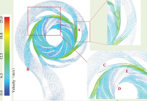
Figure 15 enlarges the partial field to reveal the vortices in area E and D, and backflow in area C. Because of the relative position between impeller and RGVs, the velocity direction out of the impeller in area E does not point to the guide vane in the downstream. As a result, backflow appears in the guide vane channel of area C, which blocks the local flow and further leads to the lower velocity in the impeller passage upstream and thus the vortices formations at regions D and E.

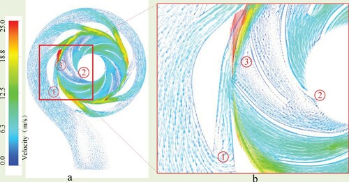
The same phenomenon happened in Case CL1, as shown in Figure 16. The downstream backflow appeared in region 1, and the lower velocity showed in region 3 and the vortex appeared in region 2 in the impeller.

Figure 16. Velocity vectors in impeller and volute domains of CL1 with marks $◯1$, $◯2$, $◯3$.

The above velocity field analysis about the five clocking positions explains the discrepancies of the pump head under the design condition. The impact of the fluid out of the RGVs on the volute wall, the downstream backflow together with eddies in the impeller passage are the two main causes. They are the reasons why the pump head of the case CL4 has minimal value, followed by CL0 and CL1. Hence, the optimal angle between the RGVs and the volute should avoid both the radial flow impingement on the wall and the shear flow in the circumferential direction.

3.1.3. Non-dimensional parameter α

The impeller is the only rotating part in the pump. In order to further investigate how the clocking positions of the RGVs influence the flow pattern in the impeller domain quantitatively, a non-dimensional coefficient α is first proposed, which is defined as follows: (5) $\alpha \text{ = }\frac{E(v^2)\text{ - }{E}^2(v)}{E^2(v)}$(5) where $E(v)=\sum _{i=1}^n{S}_i\ast v_i/\sum _{i=1}^n{S}_i$ is the area average of velocity; $E(v^2)=\sum _{i=1}^n{S}_i\ast v_i^2/\sum _{i=1}^n{S}_i$ is the area average of the square of velocity; $S_i$ is the area of a surface grid cell; $v_i$ is the mean velocity of the grid cell.

The parameter α is between 0 and 1. It is obvious that $E(v^2)$ is equal to $E^2(v)$ when the mean velocities of all the cell grids on the surface of the impeller outlet are the same, and at that time α is 0. The more discrepant the velocities of the surface grids are, the closer α gets to 1. Hence, the coefficient α represents the non-uniformity of the velocity field. The relationship of the non-dimensional coefficient α at the outlet surface of the impeller and the pressure head of the impeller is shown in Figure 17(a). It is found that the pressure head of the impeller is just negatively correlated to the non-uniformity of the velocity field in the impeller domain at flow rate Q_r. In other words, a higher impeller pressure head corresponds to lower factor α. The same situation is for the pump head as shown in Figure 19(b).

Figure 17. Comparison of the velocity coefficient and the pressure head.

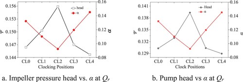
The above analysis indicates that the clocking position of the RGVs will affect the velocity homogeneity of the outlet surface of the impeller, and further influence the hydraulic characteristics of the pump.

3.2. Unsteady analysis

The unsteady simulation is initialized with the pressure and velocity fields of steady calculation in each case. The sliding meshes are adopted to simulate the rotor-stator interaction. The rotating speed is constant for all cases. Unsteady computation focuses on the pressure fluctuation and force pulsation at different locations of RGVs.

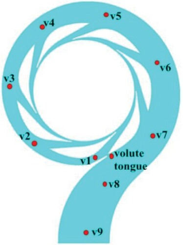
For unsteady analysis of pressure fluctuations, 10 monitoring points are set in the volute domain as shown in Figure 18.

Figure 18. Locations of the monitoring points in the volute (CL0 is taken as the example of the diagram).

Firstly, the evolution of pressure fluctuations in a period at the volute tongue is analysed at design rated flow with 5 different clocking positions (see Figure 21). There are five obvious trough-peaks in one period due to the rotor-stator interaction. In comparison with the other four cases, Case CL2 has minimal pressure fluctuation. Moreover, the pressure-fluctuation range of Case CL1 is the widest, followed by CL3. In a word, CL2 has the best performance in terms of the pressure fluctuation near the volute tongue (Figure 19).

Figure 19. Pressure fluctuations of the volute tongue at the design rated flow.

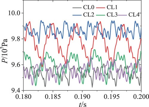
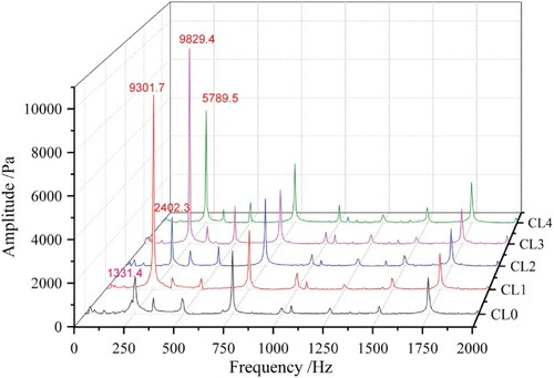
Figure 20 shows the frequency spectra of pressure fluctuation on point V9 at five clocking cases at design rated conditions. The BPF (250 Hz), third order of BPF (750 Hz), and the seventh order of BPF (1750 Hz) are the dominant frequencies corresponding to the numbers of impeller blades, inlet guide vanes, and outlet guide vanes, respectively. It proves the rotor-stator interaction is the main reason for pressure fluctuation in the pump. The most obvious differences between the five clocking positions are the enormous amplitude discrepancies at the BPF point (250 Hz). It is 1331.4 Pa for Case CL0, while it reaches up to 9829.4 Pa for Case CL3. The amplitudes of other frequency peaks are almost the same between the five cases. It demonstrates that the clocking effect mainly affects the amplitude of the blade passing frequency of pressure pulsations.

Figure 20. Frequency spectra of Pressure fluctuations on point V9 (outlet) at Qr.

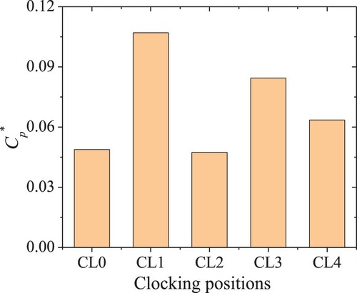
The statistical analysis is adopted to quantify the differences in pressure fluctuation. The non-dimensional pressure coefficient (C_p) is defined: $C_p=(p-\overline{p})/0.5\rho {\text{u}}^2$. In order to express the average pressure coefficient and pressure fluctuation intensity, $\overline{{\text{C}}_{\text{p}}}$ and ${\text{C}}_{\text{p}}^{\ast }$ are defined in Equations (6) and (7) (Liu et al., 2013), where u is the tangential speed of the impeller, and T is the rotating period of the impeller. Figure 21 shows the pressure fluctuation intensity at the volute tongue at different clocking positions. The lowest pressure fluctuation intensity is at CL2, and the highest intensity appears at CL1. (6) $\begin{array}{rl}\overline{C_p}& =\frac{1}{N}\sum _{n=1}^N{C}_p\left(x,y,z,\frac{n}{360}T\right)N=360\end{array}$(6) (7) $\begin{array}{rl}{C}_p^{\ast }& =\sqrt{\frac{1}{N}\sum _{n=1}^N{(C_p(x,y,z,\frac{n}{360}T)-\overline{C_p})}^2}N=360\end{array}$(7)

Figure 21. Pressure fluctuation intensity at volute tongue.

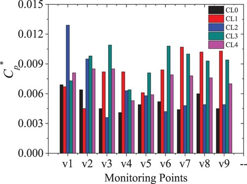
The pressure fluctuation intensities at the nine monitoring points of the volute are shown in Figure 22. The pressure fluctuation intensity of Case CL2 is generally decreasing from point v1 to v9 despite point v3. It has the minimal value at points v3, v6, and v8. In comparison with other cases, Case CL0 has the smallest values at points v4, v5, v7, and v9, and it never reaches the maximum at all monitoring points. Case CL1 has the maximum pressure fluctuation intensity at points v4, v7, v8, and v9. At monitoring points v2, v3, v5, and v6, the maximum pressure fluctuation intensity appears at the clocking position CL3. For Case CL4, the pressure fluctuation intensity at any monitoring point is neither the maximum nor the minimum. As a whole, CL0 and CL2 perform relatively well in terms of the pressure fluctuation intensity.

Figure 22. Pressure fluctuation intensities in the volute domain.

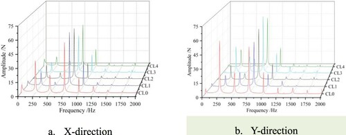
The clocking effect on the radial hydraulic forces on the impeller is also investigated. Figure 23 shows the frequency spectrums of the radial forces at the X-direction and Y-direction. As seen, the dominant frequencies are the third order of the BPF for five cases as the inducer has three vanes. It is the BPF whose amplitudes change dramatically in the different clocking positions for both X and Y directions. Hence, the clocking effect has the same effect on the radial force as the pressure pulsation. Case CL0 has the worst behavior as it has the highest amplitude of BPF in both X and Y direction, and the CL3 comes second. Comprehensively speaking, CL2 performances best, followed by CL1.

Figure 23. Frequency spectra of radial forces.

To sum up, the clocking positions of the outlet RGVs, with high curvature of the suction side of vanes, have a great effect on the pulsating pressure and radial forces, as illustrated in the above figures. In comparison with the other four cases, Case CL2 of 20° clocking angle has comprehensive dynamic behaviors as it has the lowest force pulsation. In that case, it is less possible for the pump to have some dramatic fluid transients, such as cavitation (Cheng et al., 2019), and also beneficial to the rotor radial force as it can diminish the interaction between the case and vanes (Alemi et al., 2015).

4. Conclusions

In the study, the clocking effect of the outlet RGVs on the hydrodynamic characteristics of a centrifugal pump with both inlet and outlet guide vanes is numerically investigated for the first time and experiments have verified the correctness and reliability of the computation for both steady and unsteady conditions. The head, hydraulic efficiency, the pressure, and radial force pulsation of the pump influenced by five clocking positions are studied specifically. The conclusions are as follows:

1. The pump model has the optimal hydrodynamic performance when the installation angle between the RGVs and the volute tongue is 20^o. Compared to the design angle, it can increase the pump head by 6.9% and the efficiency by 4.4%. It indicates the pump has better hydraulic behavior when the volute tongue is right in the middle of the two vanes.

2. The RGVs clocking position affects the velocity direction of fluid out of the vanes, and the improper angle will result in flow impacts on the volute wall, backflows in the outlet of the RGVs, and vortices near the inlet of the blades. All three factors influence the velocity distribution of the impeller and further weaken the hydraulic performance of the pump.

3. The clocking position of the outlet RGVs mainly affects the amplitude of the blade passing frequency (BPF) in the pressure pulsations and radial forces, and it has a slight impact on other hydraulic frequencies for the single-stage pump studied in the paper.

4. In addition, the clocking position of the outlet RGVs has little impact on the function of the inlet inducer. Amplitudes of the third harmonic of BPF, which is related to the inlet inducer, remain almost unchanged in different positions.

All the findings will be valuable and instructive for the designers to pick up the optimal position of the outlet RGVs relative to the volute tongue in comprehensive consideration of optimization of the pump head, efficiency, pressure fluctuation, and radial forces.

5. Improvements and future direction

However, there are several imperfections in the paper. Due to many practical difficulties and restrictions, only the confirmatory experiments of Case CL0 are conducted. Second, it will be more convincing if the pressure pulsation of the tongue and volute can be detected and compared with the calculation, not just for the design condition. In a word, more validated experiments need to be carried out with more sensors to evaluate the clocking effect of outlet RGVs and its effect on the cavitation resistance of the pump. If possible, visualization measurement of the flow field inside the pump in laboratory conditions will also be a hotspot of future work.

Disclosure statement

No potential conflict of interest was reported by the author(s).

Additional information

Funding

This work was supported by the National Natural Science Foundation of China [Grant number 51806042], China Postdoctoral Science Foundation [grant number 2018T110273].

References

- Abadi, E., Sadi, A. M., Farzaneh-Gord, M., Ahmadi, M., Kumar, M. H., & Chau, R., & W, K. (2020). A numerical and experimental study on the energy efficiency of a regenerative heat and mass exchanger utilizing the counter-flow Maisotsenko cycle. Engineering Applications of Computational Fluid Mechanics, 14(1), 1–12. https://doi.org/https://doi.org/10.1080/19942060.2019.1617193
- Alemi, H., Nourbakhsh, S. A., Raisee, M., & Najafi, A. F. (2015). Development of new “multivolute casing” geometries for radial force reduction in centrifugal pumps. Engineering Applications of Computational Fluid Mechanics, 9(1), 1–11. https://doi.org/https://doi.org/10.1080/19942060.2015.1004787
- Barrio, R., Fernandez, J., Blanco, E., & Parrondo, J. (2011). Estimation of radial load in centrifugal pumps using computational fluid dynamics. European Journal of Mechanics B-Fluids, 30(3), 316–324. https://doi.org/https://doi.org/10.1016/j.euromechflu.2011.01.002
- Behr, T., Porreca, L., Mokulys, T., Kalfas, A. I., & Abhari, R. S. (2006). Multistage aspects and unsteady effects of stator and rotor clocking in an axial turbine with low aspect ratio blading. Journal of Turbomachinery-Transactions of the Asme, 128(1), 11–22. https://doi.org/https://doi.org/10.1115/1.2101855
- Chao, Q., Zhang, J. H., Xu, B., Huang, H. P., & Zhai, J. (2019). Effects of inclined cylinder ports on gaseous cavitation of high-speed electro-hydrostatic actuator pumps: A numerical study. Engineering Applications of Computational Fluid Mechanics, 13(1), 245–253. https://doi.org/https://doi.org/10.1080/19942060.2019.1576545
- Cheng, X., Li, Y., & Zhang, S. (2019). Effect of inlet sweepback angle on the cavitation performance of an inducer. Engineering Applications of Computational Fluid Mechanics, 13(1), 713–723. https://doi.org/https://doi.org/10.1080/19942060.2019.1640134
- Dash, N., Roy, A. K., & Kumar, K. (2018). Design and optimization of mixed flow pump impeller blades – A review. Materials Today-Proceedings, 5(2), 4460–4466. https://doi.org/https://doi.org/10.1016/j.matpr.2017.12.015
- Deng, J., Jin, L., Yi, R., Feng, J.-J., & Luo, X.-Q. (2016). Effect of clocking position of front guide vane on pulsation characteristic of pressure in centrifugal pump. Journal of Northwest A & F University. https://doi.org/https://doi.org/10.13207/j.cnki.jnwafu.2016.01.032
- Dieter, B., Sabine, A., & Jing, R. (2005). Investigation of the optimum clocking position in a two-stage axial turbine. International Journal of Rotating Machinery. https://doi.org/https://doi.org/10.1155/IJRM.2005.202
- Haldeman, C. W., Dunn, M., Barter, J. W., Green, B. R., & Bergholz, R. F. (2005). Experimental investigation of vane clocking in a one and one-half stage high pressure turbine. Journal of Turbomachinery-Transactions of the Asme, 127(3), 512–521. https://doi.org/https://doi.org/10.1115/1.1861915
- Jiang, W., Li, G., Liu, P.-F., & Fu, L. (2016). Numerical investigation of influence of the clocking effect on the unsteady pressure fluctuations and radial forces in the centrifugal pump with vaned diffuser. International Communications in Heat and Mass Transfer, 71, 164–171. https://doi.org/https://doi.org/10.1016/j.icheatmasstransfer.2015.12.025
- Key, N. L. (2014). Compressor vane clocking effects on embedded rotor performance. Journal of Propulsion and Power, 30(1), 246–248. https://doi.org/https://doi.org/10.2514/1.B34604
- Liu, H., Cui, J., Tan, M., Wu, X., & Xu, H. (2013). CFD calculation of clocking effect on centrifugal pump. Transactions of the Chinese Society of Agricultural Engineering, 29(14), 67–73. https://doi.org/https://doi.org/10.3969/j.issn.1002-6819.2013.14.009
- Menter, F. R. (1994). Two-equation eddy-viscosity turbulence models for engineering applications. AIAA Journal, 32(8), 1598–1605. https://doi.org/https://doi.org/10.2514/3.12149
- Munih, J., Hocevar, M., Petric, K., & Dular, M. (2020). Development of CFD-based procedure for 3d gear pump analysis. Engineering Applications of Computational Fluid Mechanics, 14(1), 1023–1034. https://doi.org/https://doi.org/10.1080/19942060.2020.1789506
- Pinto, R. N., Afzal, A., D’Souza, L. V., Ansari, Z., & Samee, A. D. M. (2017). Computational fluid dynamics in turbomachinery: A review of state of the art. Archives of Computational Methods in Engineering, 24(3), 467–479. https://doi.org/https://doi.org/10.1007/s11831-016-9175-2
- Qu, W., Tan, L., Cao, S., Wang, Y., & Xu, Y. (2016). Numerical investigation of clocking effect on a centrifugal pump with inlet guide vanes. Engineering Computations, 33(2), 465–481. https://doi.org/https://doi.org/10.1108/ec-12-2014-0259
- Ramezanizadeh, M., Alhuyi Nazari, M., Ahmadi, M. H., & Chau, K. W. (2019). Experimental and numerical analysis of a nanofluidic thermosyphon heat exchanger. Engineering Applications of Computational Fluid Mechanics, 13(1), 40–47. https://doi.org/https://doi.org/10.1080/19942060.2018.1518272
- Saren, V. E., Savin, N. M., Dorney, D. J., & Zacharias, R. M. (1998). Experimental and numerical investigation of unsteady rotor-stator interaction on axial compressor stage (with IGV) performance. Second international conference EAHE. https://doi.org/https://doi.org/10.1007/978-94-011-5040-8_27
- Shah, S. R., Jain, S. V., Patel, R. N., & Lakhera, V. J. (2013). CFD for centrifugal pumps: A review of the state-of-the-art. Chemical, Civil and Mechanical Engineering Tracks of 3rd Nirma University International Conference on Engineering (Nuicone2012), 51, (pp. 715–720).
- Shuai, Z.-J., Li, W.-Y., Zhang, X.-Y., Jiang, C.-X., & Li, F.-C. (2014). Numerical study on the characteristics of pressure fluctuations in an axial-flow water pump. Advances in Mechanical Engineering. https://doi.org/https://doi.org/10.1155/2014/565061
- Si, Q., Ali, A., Yuan, J., Fall, I., & Yasin, F. M. (2019). Flow-induced noises in a centrifugal pump: A review. Science of Advanced Materials, 11(7), 909–924. https://doi.org/https://doi.org/10.1166/sam.2019.3617
- Smith, N. R., & Key, N. L. (2013). Vane clocking effects on stall margin in a multistage compressor. Journal of Propulsion and Power, 29(4), 891–898. https://doi.org/https://doi.org/10.2514/1.B34636
- Staeding, J., Wulff, D., Kosyna, G., Becker, B., & Guemmer, V. (2012). An experimental investigation of stator clocking effects in a two-stage low-speed axial compressor. Proceedings of the Asme Turbo Expo 2011, 7, 1563–1574. https://doi.org/https://doi.org/10.1115/GT2011-45680
- Suh, J. W., Yang, H. M., Kim, Y. I., Lee, K. Y., Kim, J. H., Joo, W. G., & Choi, Y. S. (2019). Multi-objective optimization of a high efficiency and suction performance for mixed-flow pump impeller. Engineering Applications of Computational Fluid Mechanics, 13(1), 744–762. https://doi.org/https://doi.org/10.1080/19942060.2019.1643408
- Tan, M., He, X., Liu, H., Dong, L., & Wu, X. (2016). Design and analysis of a radial diffuser in a single-stage centrifugal pump. Engineering Applications of Computational Fluid Mechanics, 10(1), 500–511. https://doi.org/https://doi.org/10.1080/19942060.2016.1210027
- Tan, M., He, N., Liu, H., Wu, X., & Ding, J. (2016). Experimental test on impeller clocking effect in a multistage centrifugal pump. Advances in Mechanical Engineering, 8, 4. https://doi.org/https://doi.org/10.1177/1687814016644376
- Walker, G. J., & Oliver, A. R. (1972). The effect of interaction between wakes from blade rows in an axial flow compressor on the noise generated by blade interaction. Journal of Engineering for Gas Turbines & Power, 94(4), 241–248. https://doi.org/https://doi.org/10.1115/1.3445679
- Wang, W., Pei, J., Yuan, S., & Yin, T. (2018). Experimental investigation on clocking effect of vaned diffuser on performance characteristics and pressure pulsations in a centrifugal pump. Experimental Thermal and Fluid Science, 90, 286–298. https://doi.org/https://doi.org/10.1016/j.expthermflusci.2017.09.022