Coupled heat transfer model for the combustion and steam characteristics of coal-fired boilers

Abstract

This paper presents a coupled heat transfer model for coal-fired boilers that integrates boiler’s fire side computational fluid dynamics (CFD) solution with the boiler’s steam cycle, and thus, can predict the boiler steam temperatures subject to different boiler design and operation conditions. In this coupled model, the heat transfer submodels describing the gas-steam heat exchange for each part of boiler heating surfaces are integrated by exchanging the steam temperatures iteratively. This coupled heat transfer model is self-consistent since it ensures the fire side heat transfer solution to always coincide with the steam temperature changes across each boiler heating surface. This model is specifically designed to provide efficient computational solutions to engineering boiler problems in which the changes of boiler steam temperatures subject to different boiler design and operation conditions are of the major concerns. This model is applied to a 320 MW subcritical boiler to evaluate the impacts of coal switching and boiler operation adjustment on boiler’s heat transfer distributions and steam temperatures. The simulation results demonstrate that this model can effectively capture the complex coupled heat transfer behavior between the fire and steam sides of boiler and serve as an efficient predictive tool for engineering boiler problems.

KEYWORDS:

• Pulverized coal boiler
• coal combustion
• coupled simulation
• heat transfer
• steam temperature

1. Introduction

Coal-fired power plants contributed approximately 38% of world power generation in 2018 (BP Statistical Review of World Energy, www.bp.com/statisticalreview, 2019). This stimulated the development of computational fluid dynamics (CFD) boiler models as predictive tools to evaluate various boiler design and operation optimization options to improve thermal efficiency and reduce pollutant emissions of coal-fired boilers. Boiler CFD has been employed to study a wide range of boiler problems, such as low NO_x combustion optimization (Adamczyk et al., 2014; Backreedy et al., 2005; Diez et al., 2008; Tan et al., 2017; Zhang et al., 2015), tube surface erosion (Gandhi et al., 2012), high-temperature corrosion (Yang et al., 2017), coal switching (Spitz et al., 2008), gas temperature deviation (Tan et al., 2018; Yin et al., 2002), slagging and fouling (Lee & Lockwood, 1999; Weber et al., 2013), and the development of advanced heat exchangers (Abadi et al., 2020; Ramezanizadeh et al., 2019). Nevertheless, CFD boiler models are still highly deficient in predicting boiler steam parameters subject to different boiler design and operation conditions.

A boiler is, first of all, a steam generator. Steam parameters, such as superheat (SH) and reheat (RH) steam temperatures, always play a central role in the operation of boilers. Potential impacts on steam temperatures are of major concern in many boiler design and operation optimization applications. For example, during recent years, many of the coal power plants in the US have switched from eastern bituminous coals to Powder River Basin (PRB) coals in order to reduce SO₂ and NO_x emissions. However, since eastern bituminous coals usually have much higher heating values (∼30 MJ/kg) than those of PRB coals (∼20 MJ/kg), the heat transfer distribution in boilers has changed dramatically. This has led to significant changes in steam temperatures and many boilers have thus suffered from over-heated steam or even having to de-rate unless costly modifications to the boiler heating surfaces had also been implemented. Moreover, most modern boilers have installed overfire air (OFA) systems to allow for staging combustion to reduce NO_x emissions. Staging combustion, however, delays fuel combustion, and thus may significantly affect boiler heat transfer distribution and steam temperatures. All these problems encountered in boiler applications necessitate CFD boiler models developing the capability of predicting steam temperatures when subjected to different boiler design and operation conditions.

CFD models, in which the gas phase conservation equations are solved in the boiler fire side domain, generally do not include the steam cycle of the boiler. Recently, a few studies have coupled three-dimensional (3D) CFD models with one-dimensional (1D) process models that describe boiler steam cycles. Specifically, Laubscher and Rousseau (Laubscher & Rousseau, 2019a, 2020; Rousseau & Laubscher, 2020) integrated the CFD model developed under ANSYS® Fluent® (fluid simulation software—https://www.ansys.com/products/fluids/ansys-fluent) with the 1D process model Flownex® (simulation environment—https://flownex.com/). The coupling interface between the two models is the external surface of the heat exchanger. Flownex receives heat flux solutions from Fluent and calculates the internal heat transfer coefficients and steam temperatures in the tubes, which will then be sent back to Fluent as the thermal boundary conditions. Both models run intermittently until converged solutions are obtained. This coupled model was used to investigate the heat transfer of a subcritical boiler burning high-ash coal at varying loads and satisfactory results were obtained. Similarly, Edge et al. (2011, 2012, 2013) developed a coupled model by integrating ANSYS Fluent with a process simulator, gRPOMS (process engineering software—https://www.psenterprise.com/products/gproms). The data exchange between the two models was conducted in a way similar to that of Laubscher & Rousseau (Laubscher & Rousseau, 2019a, 2020; Rousseau & Laubscher, 2020). Liu et al. (2019, 2020) combined ANSYS Fluent with an in-house code. The heat flux distributions from Fluent were used to derive a thermal deflection curve along the furnace height. This curve was then used by the in-house code to calculate the steam and wall temperatures. Schuhbauer et al. (2014) presented a detailed coupled model in which ANSYS Fluent was integrated with the commercial software APROS (advanced process simulation software—https://www.fortum.com/products-and-services). In this model, Fluent exports a boiler’s fire side heat flux data in text files. These text files are processed by MATLAB® (The MathWorks—https://www.mathworks.com/products/matlab.html) and then exported to APROS. APROS uses this heat flow data to calculate the inner tube temperatures of boiler heating surfaces, which will then be used by Fluent as wall thermal boundary conditions. Chen et al. (2019) integrated ANSYS Fluent with COMSOL-Multiphysics (software for multiphase simulation—www.comsol.com) and simulated the coupled heat transfer of the pendant superheater of a 1000 MW supercritical boiler. Text files were used to exchange the heat flux and temperature data between the two softwares. Rather than using text files to communicate the data, Park et al. (2010) combined ANSYS CFX (CFD software program solutions—https://www.ansys.com/products/fluids/ansys-cfx) with a 1D process model, PROATES Off-Line, and the boiler heat flux and steam temperature data from the two models were exchanged through a graphical user interface (GUI).

It is seen that these integrated CFD-process models (Chen et al., 2019; Edge et al., 2011, 2012, 2013; Laubscher & Rousseau, 2019a, 2020; Liu et al., 2019, 2020; Park et al., 2010; Rousseau & Laubscher, 2020; Schuhbauer et al., 2014) coupled the boiler’s fire side and steam side solutions, and thus were able to provide steam properties in the boiler’s heating surfaces. However, since the fire and steam sides of the boilers were modeled by two different software packages, the results from the two models had to be taken as boundary conditions for each other and an interface needed to be developed to exchange the data between the 3D CFD and 1D process models. This dramatically increased the complexity of the problem and inhibited the models from being readily applied to engineering boiler problems. As a result, these integrated models were limited only to the study of steam properties in part of a boiler’s steam cycle and were unable to predict the steam temperatures along the entire steam cycle under different boiler design and operation conditions. For many boilers that are experiencing major design or operation modifications, such as coal switching and combustion system retrofit, one of the major concerns is usually whether the boilers can still maintain their designated steam temperatures, since these directly impact the thermal performance of a boiler. For these boiler applications, the overall heat transfer to each part of a boiler’s heating surfaces is sufficient to predict the change of steam temperatures, and detailed steam properties along the steam cycle are generally not required. For this reason, an alternative method is proposed in the present study in which a boiler’s fire side CFD solution and the steam temperatures are coupled all within the framework of 3D CFD model without resort to a process model for the boiler’s steam cycle. Since the heat transfer to any part of boiler’s heating surfaces affects the steam temperatures at all the downstream heating surfaces of the steam cycle that may locate upstream of the gas flow path, the boiler steam temperatures are determined by the coupled heat transfer behavior between the entire fire side and steam cycle of the boiler. For this reason, in the coupled model presented in this study, the heat transfer submodels for the furnace water wall and all the convective heat exchangers are integrated by exchanging the steam temperatures iteratively. This coupled heat transfer model is complementary to integrated CFD–process models (Chen et al., 2019; Edge et al., 2011, 2012, 2013; Laubscher & Rousseau, 2019a, 2020; Liu et al., 2019, 2020; Park et al., 2010; Rousseau & Laubscher, 2020; Schuhbauer et al., 2014). CFD–process models provide more detail on the steam properties in a single boiler heating surface, but approximations are generally made in the 3D CFD solutions to adapt the 3D results to the 1D model, while in the present model the 3D CFD results remain intact and approximations are made on the steam side in that each boiler heating surface is represented with an averaged steam temperature. Chen et al. (2019) compared different coupling schemes and found that the overall heat transfer results using averaged steam temperatures were in very close agreement with the fully coupled method that considers detailed steam properties along the steam flow. Laubscher and Rousseau (2020) also used averaged steam temperature in the coupled simulation and the heat transfer results agreed very well with the experiment data. This is the rationale behind the coupled model presented in this paper. In this way, the coupled calculation procedure is dramatically simplified and, in particular, can be realized within single CFD software without compromising much on the prediction accuracy. Moreover, as a result of the simplified procedure, the present model is able to couple the CFD solution with the entire steam cycle including the furnace water wall, superheaters, reheaters and economizers. This makes it possible for the present model to conduct efficient engineering evaluations of the potential effects of various boiler operation and retrofit options (such as coal switching, OFA system installation and heating surface modification) on the steam temperatures.

In the following, a 320 MW tangentially-fired (T-fired) subcritical boiler is first described along with its detailed operating parameters. Then the mathematical models employed in the present study are briefly introduced, after which the coupled heat transfer model is described in detail. This coupled model is first validated by the operating parameters of the 320 MW boiler and then employed to investigate some problems of wide practical interest, such as coal switching and burner setting adjustments, to demonstrate its capability as a powerful and efficient predictive tool for engineering boiler problems.

2. Boiler specification

2.1. Furnace geometry

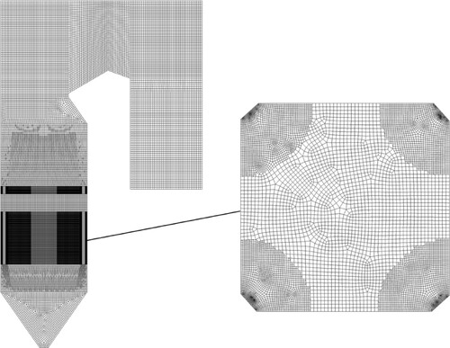
The furnace is approximately 14 m deep and wide and 56 m high. As seen in Figure 1, the platen superheater (PLSH) and division panel superheater (DPSH) are located at the upper furnace, around which part of the furnace wall is used as the wall reheater (WRH). The CFD model in this paper needs to consider the coupled heat transfer of the entire steam cycle. Thus, the furnace geometry includes the entire convection pass of boiler in which the reheaters (CRH, HRH), the superheaters (SSH, PSHs) and the economizer (ECON) are placed sequentially. The computational mesh is composed of 3.54 million hexahedral cells with the near-burner region further refined, as seen in Figure 2.

Figure 1. Schematic of the 320 MW T-fired boiler (DPSH: division panel superheater; PLSH: platen superheater; WRH: wall reheater; CRH: cold reheater, HRH: hot reheater; SSH: secondary superheater; PSH: primary superheater; ECON: economizer; SOFA: separated overfire air; Aux: auxiliary air).

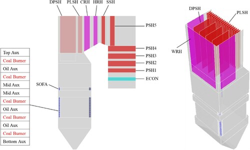
Figure 2. Side and top views of the furnace mesh distribution.

2.2. Boiler steam cycle

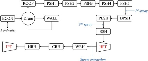
The boiler steam cycle is shown schematically in Figure 3. Feedwater enters the unit through the economizer and is then discharged to the drum. The water separated in the drum is recirculated to the furnace water wall (WALL) and the separated steam goes to the superheater. The superheater is composed of five basic components: the steam cooled roof (ROOF); the primary superheaters (PSH1–PSH5); the DPSH; the PLSH; and the secondary (final) superheater (SSH). The ROOF section includes the furnace roof and the enclosure wall of the boiler’s vertical convection pass. As seen in Figure 3, the steam from the drum enters the superheater first through the ROOF and then passes the superheaters in the sequence PSH1, PSH2, PSH3, PSH4, PSH5, DPSH, PLSH and SSH. Two stages of spray attemperators are located before the DPSH and the SSH, respectively. Superheated steam from the final superheater (SSH) is then discharged to the high-pressure turbine (HPT). After passing the HPT, the steam flow is returned to the reheaters with part of it extracted to heat the feedwater. The reheat steam passes through the reheaters in the sequence wall reheater (WRH), cold reheater (CRH) and hot reheater (HRH). Then the reheated steam goes to the intermediate-pressure turbine (IPT).

Figure 3. Schematic of the boiler’s steam cycle.

2.3. Coal property data and boiler operating data

Tables 1 and 2 give the coal property data and boiler operating data, respectively, for the model cases of the present study. The steam parameters of Case 1 are given in Table 3. All the operating data of Case 1 were taken from the plant control system. These data can be used to validate the heat transfer prediction results of the CFD model. Cases 2–4 are coal switching cases in which a coal (coal B) with reduced heating value is used. The boiler heat input, however, is kept the same for all cases. Thus, as seen in Table 2, the coal flow rates of Cases 2–4 are higher than those of Case 1. It will be seen that coal switching may result in a considerable increase of the final superheat (SH) and reheat (RH) steam temperatures. Case 3 studies the influence of spray attemperation on the steam temperatures in order to examine if spray can recover the steam temperatures to their original values. In Case 4, the injection direction of the coal and air streams are biased downwards by 15° by tilting the burners. This is another attempt to recover the steam temperatures of the boiler after coal switching. The total air flow rate (355 kg/s) and air partition between the primary air, secondary air and overfire air (23.6/61.4/15.0%) are kept the same for all cases.

Table 1. Summary of coal property data (as received).

	Coal A	Coal B
Moisture, %	7.50	19.30
Ash, %	15.16	11.41
Volatile, %	28.63	25.64
Fixed carbon, %	48.71	43.65
C, %	63.24	52.47
H, %	4.08	2.84
O, %	8.46	13.23
N, %	0.75	0.34
S, %	0.81	0.41
Lower heating value, MJ/kg	24.58	19.00

Table 2. Summary of main operating data for model cases.

Model case	1	2	3	4
Coal flow rate, kg/s	34.3	44.4
Spray flow rate, kg/s	–	–	6.67	–
Burner tilt angle, degrees	–	–	–	−15.0

Table 3. Summary of boiler feedwater and steam parameters (Case 1).

Superheat/reheat steam flow rates, kg/s	295.8/268.1
Feedwater/drum/superheat pressures, MPa·g	20.30/19.91/18.54
Reheat steam inlet/outlet pressures, MPa·g	4.53/4.30
Feedwater/ECON outlet temperatures, °C	261.0/281.0
PSH/DPSH/PLSH/SSH outlet steam temperatures, °C	410.0/450.0/509.0/543.0
Reheater inlet steam temperature, °C	345.8
WRH/CRH/HRH outlet steam temperatures, °C	396.0/488.0/543.0

3. Mathematical models

The CFD model described in the present study is implemented within the framework of ANSYS® Fluent® (Version 13). The realizable k–ϵ model is used to model the turbulence. Lagrangian stochastic model is used to track the trajectories of 129,700 coal particles of average diameter 59 µm. The PSIC method is used to account for the mass, energy and momentum exchange between the coal particles and the gas phase flow (Boyd & Kent, 1988; Lockwood et al., 1980; Truelove, 1984). The radiation heat transfer is simulated by the discrete ordinate method. The single reaction rate model (Badzioch & Hawksley, 1970) is used to model the coal devolatilization with the rate parameters determined by PC Coal Lab® software as a pre-processor (Niksa, 1995; Park et al., 2013). Note that V₀ in Table 4 is the total coal volatile yield under high heating rate, which is higher than the volatile content of coal proximate analysis data in Table 1.

Table 4. Coal devolatilization rate parameters.

	Coal A	Coal B
V0, %	43.70	36.03
Av, s^−1	9,203	3,447
Ev, J/mole	27,670	16,960

The volatile matter is represented by a fictitious species C_aH_bO_cS_dN_e with each of its components determined from the coal data shown in Tables 1 and 4 (Boyd & Kent, 1988). The combustion reaction of the volatile is modeled by a two-step global mechanism (Backreedy et al., 1999; Hu et al., 2014): (1) $\begin{array}{rl}& {\text{C}}_a{\text{H}}_b{\text{O}}_c{\text{S}}_d{\text{N}}_e+\left(\frac{a}{2}+\frac{b}{4}-\frac{c}{2}+d\right){\text{O}}_2\\ & \to a\text{CO}+\frac{b}{2}{\text{H}}_2\text{O}+d\text{S}{\text{O}}_2+\frac{e}{2}{\text{N}}_2\end{array}$(1) (2) $\begin{array}{rl}& \text{CO}+\frac{1}{2}{\text{O}}_2\to \text{C}{\text{O}}_2.\end{array}$(2)

The turbulent reaction rates of the combustion reactions are calculated by the eddy dissipation model (Magnussen & Hjertager, 1977). The heterogeneous reaction rate of char (3) ${\text{C}}_{\text{char}}+\frac{1}{2}{\text{O}}_2\to \text{CO}$(3) is modeled using the Baum and Street model (Baum & Street, 1971). The rate parameters for the char reaction model are A_c = 0.001 kg/(m² s atm) and E_c = 79.0 kJ/mole. The value of E_c is obtained from the averaged measurement values for high-volatile bituminous coals made in an entrained reactor (Mitchell et al., 1992). The value of A_c is obtained based on the calibration calculation with the plant flyash unburned carbon data. The above models have been introduced in many research articles (Laubscher & Rousseau, 2019b; Lockwood et al., 1980; Park et al., 2013; Wang et al., 2020) and will not be described in much detail here.

4. Coupled heat transfer model

4.1. Heat transfer models

The heat transfer models for the furnace wall and convective heat exchangers of coal-fired boilers have been introduced in detail in Wang et al. (2020). Here, we give only a brief introduction to these models and place the emphasis on the coupled calculation procedure. The heat flux q of furnace wall coated with ash deposit layer is calculated by (4) $q={\mathcal{H}}_{\text{ext}}(T_{\text{w}}-T_{\text{s}}),$(4) where ${\mathcal{H}}_{\text{ext}}$ is the wall heat transfer coefficient, $T_{\text{w}}$ the surface temperature of the wall ash layer, and $T_{\text{s}}$ the temperature of water/steam. Equation (4) defines the thermal boundary conditions of the wall with ${\mathcal{H}}_{\text{ext}}$ and $T_{\text{s}}$ given as the input parameters (Laubscher & Rousseau, 2019b; Wang et al., 2020). For subcritical boilers, the value of $T_{\text{s}}$ takes the value of saturated steam temperature (∼366°C) at drum pressure. As discussed in detail in Wang et al. (2020), the value of ${\mathcal{H}}_{\text{ext}}$ depends on the actual wall slagging status of the boiler. It can be determined based on the plant data through a validation calculation. In the validation process, the specific enthalpies of saturated steam and water out of the economizer, $h_{\text{sat},v}$ and $h_{\text{econ}}^{\text{out}}$, can be determined according to the steam operating data of the boiler. They, along with the feedwater flow rate ${\dot{m}}_{\text{feed}}$, are then used to estimate the heat absorption of the furnace wall $Q_{\text{wall}}^{DCS}$: (5) $Q_{\text{wall}}^{DCS}={\dot{m}}_{\text{feed}}(h_{\text{sat},v}-h_{\text{econ}}^{\text{out}}).$(5)

The heat absorption of the furnace wall from the CFD solution can be calculated by integrating the predicted wall heat fluxes over the entire wall surface, $Q_{\text{wall}}={\int }_{\text{wall}}^{}q\text{d}A.$ Then the value of ${\mathcal{H}}_{\text{ext}}$ can be fine-tuned until the CFD solution $Q_{\text{wall}}$ matches the value of $Q_{\text{wall}}^{DCS}$ from Equation (5). In this way, the boiler’s actual wall slagging condition can be considered accurately in the definition of ${\mathcal{H}}_{\mathrm{ext}}$.

The convective heat exchangers of the boiler are represented by porous volumes in the geometry (Diez et al., 2008; Laubscher & Rousseau, 2019b; Schuhbauer et al., 2014; Tan et al., 2017; Wang et al., 2020; Yin et al., 2002). Their heat absorption is calculated by (6) $q_{\text{conv}}=S_{\text{conv}}\psi {\mathcal{H}}_{\text{f}}(T_{\text{f}}-T_{\text{s}}),$(6) where $q_{\text{conv}}$ and $S_{\text{conv}}$ are the amount of heat transfer and tube outer area of the heat exchanger per unit volume, respectively, ${\mathcal{H}}_{\text{f}}$ denotes the fire side heat transfer coefficient of the heat exchanger, $\psi$ is the thermal effectiveness factor, and $T_{\text{f}}$ is the flue gas temperature (Che, 2008; Wang et al., 2020). The values of $\psi$ depend on the actual fouling condition of the heat exchangers and, hence, can only be determined accurately by a validation calculation with the boiler operating data.

4.2. Coupled heat transfer model

It is noted that the heat exchange between the fire and steam sides of a boiler at any part of boiler heating surfaces does not occur independently. For example, if the heat transfer of PSH1 is changed, it will affect the steam temperatures in all the downstream heating surfaces along the steam cycle (e.g. the DPSH, the PLSH and the SSH), and thereby will affect the heat transfer to these heating surfaces as well. Consequently, the furnace gas temperature distribution is changed, which in turn may affect the heat transfer distribution of the entire boiler. Thus, the steam temperatures of the boiler are determined by the complex coupled heat transfer behavior between the entire gas flow and steam cycle of the boiler. For this reason, in this study the heat transfer submodels of furnace wall and convective heat exchangers are integrated by exchanging the steam temperatures iteratively. The coupled algorithm is shown schematically in Figure 4. The first step of the calculation is to conduct the CFD simulation and calculate the heat transfer to each part of the boiler heating surfaces using assumed steam temperatures. The heat absorption by furnace water wall $Q_{\text{wall}}$ evaporates the feedwater to saturated steam. Then the feedwater flow rate, ${\dot{m}}_{\mathrm{feed}}$, can be calculated according to (7) $Q_{\text{wall}}={\dot{m}}_{\text{feed}}(h_{\text{sat,}v}-h_{\text{econ}}^{\text{out}}).$(7)

Figure 4. Schematic of the coupled heat transfer calculation algorithm.

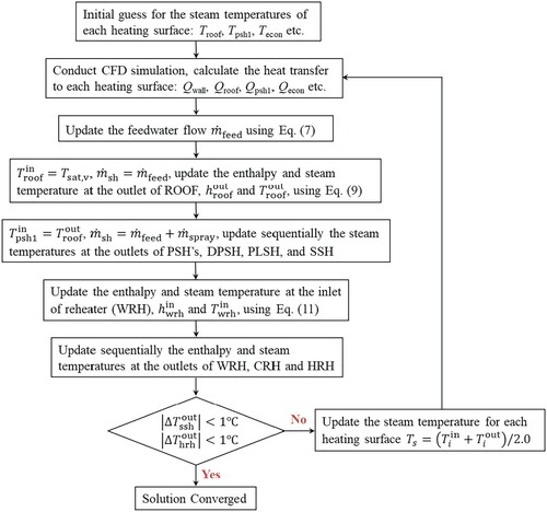
The value of ${\dot{m}}_{\text{feed}}$ is then used by the heat transfer submodels for all the downstream heating surfaces in the steam cycle. The steam leaving the drum passes through the superheaters in the sequence ROOF, PSH1–PSH5, DPSH, PLSH and SSH. In the steady state, the steam flow entering the ROOF superheater is equal to the feedwater flow, ${\dot{m}}_{\text{sh}}={\dot{m}}_{\text{feed}}$. Two stages of spray attemperators are located before the DPSH and the SSH, respectively. If an attemperating spray flow of ${\dot{m}}_{\text{spray}}$ is applied to reduce the SH steam temperature, the steam flow downstream of the attemperators (the DPSH, the PLSH and the SSH) will increase correspondingly, (8) ${\dot{m}}_{\text{sh}}={\dot{m}}_{\text{feed}}+{\dot{m}}_{\text{spray}}.$(8)

The steam entering the ROOF superheater is assumed to be at the saturated temperature, $T_{\text{sat,}v}$ (∼366°C). The heat absorption of the ROOF superheater, $Q_{\text{roof}}$, from the CFD solution is then used to calculate the specific enthalpy at its outlet, $h_{\text{roof}}^{\text{out}}$, according to (9) $Q_{\text{roof}}={\dot{m}}_{\text{sh}}(h_{\text{roof}}^{\text{out}}-h_{\text{sat,}v}).$(9)

The outlet enthalpy of the ROOF superheater is then used by its downstream heat exchanger, PSH1, as its inlet enthalpy to calculate its outlet specific enthalpy based on its heat absorption, $Q_{\text{psh}1}.$ This process repeats sequentially for the heat exchangers along the steam cycle until the specific enthalpy out of the final superheater (SSH), $h_{\text{ssh}}^{\text{out}}$, is obtained.

The SH steam out of the SSH is discharged to drive the HP turbine. The specific enthalpy of steam out of the HP turbine, $h_{\text{hp}}^{\mathrm{out}}$, can be obtained according to (10) ${\eta }_{\text{hp}}=\frac{h_{\text{ssh}}^{\text{out}}-h_{\text{hp}}^{\text{out}}}{h_{\text{ssh}}^{\text{out}}-h_{\text{hp}}^{\text{out},s}},$(10) where ${\eta }_{\text{hp}}$ is the isentropic efficiency of the HP turbine and $h_{\text{hp}}^{\text{out},s}$ is the specific enthalpy out of the HP turbine for the isentropic process. The isentropic efficiency of the HP turbine, ${\eta }_{\text{hp}}\approx 81.6\mathrm{\%}$, can be determined based on the SH and RH steam parameters from the plant operating data as listed in Table 3. The specific enthalpy of steam out of the HP turbine, $h_{\text{hp}}^{\text{out}}$, is then used as the inlet enthalpy of the reheaters, $h_{\text{wrh}}^{\text{in}}.$ Using the steam extraction rate estimated based on the SH and RH steam flow rates of the plant data, the reheat steam flow, ${\dot{m}}_{\text{rh}}$, can be determined as ${\dot{m}}_{\text{rh}}\approx 0.906{\dot{m}}_{\text{sh}}.$ The first stage of the reheaters is the wall reheater (WRH). Then the specific enthalpy of RH steam out of the WRH, $h_{\text{wrh}}^{\mathrm{in}}$, can be obtained according to (11) $Q_{\text{wrh}}={\dot{m}}_{\text{rh}}(h_{\text{wrh}}^{\text{out}}-h_{\text{wrh}}^{\text{in}}),$(11) where $Q_{\text{wrh}}$ is the heat absorption of WRH. Then, following the same procedure as that for the superheaters, the specific enthalpies of the RH steam at the outlets of the CRH and the HRH can be solved sequentially.

With the specific enthalpies at the inlets and outlets of each heating surface solved, the inlet and outlet steam temperatures, $T_i^{\text{in}}$ and $T_i^{\text{out}}$ (i = ECON, PSH1, CRH, etc.), can easily be obtained. In this way, the coupled model is self-consistent since it ensures that the gas side heat transfer results always coincide with the corresponding steam temperature changes across each boiler heating surface. Then the average steam temperature $T_{\text{s}}=(T_i^{\text{in}}+T_i^{\text{out}})/2$ can be updated for the next iteration of the calculation. The iteration repeats until the changes in the final SH and RH steam temperatures between two adjacent iterations drop below a criterion value, e.g. $|\mathrm{\Delta }{T}_{\text{ssh}}^{\text{out}}|<1^{\text{o}}\text{C}$ and $|\mathrm{\Delta }{T}_{\text{hrh}}^{\text{out}}|<1^{\circ }\text{C}$. Usually, with reasonable assumed initial values for the steam temperatures, two or three iterations are enough to obtain the converged solution.

In this coupled model, the local gas flow field from the 3D CFD solution is used to calculate the heat transfer and an approximation is made on the steam side in that each heating surface is represented with an averaged steam temperature. Usually, the steam temperature changes across the heat exchangers located at the vertical convection pass (e.g. PSHs) are rather small (as will be seen in Table 7). Thus, very little inaccuracy would be induced by using an averaged steam temperature to represent the entire heat exchanger. The steam temperature changes across the heat exchangers located upstream of the convection pass (e.g. SSH and HRH) are relatively larger. However, the temperature differences between the flue gas and steam, $T_{\text{f}}-T_{\text{s}}$, are also much larger. Thus, the relative inaccuracy induced by using average steam temperatures would remain small. Moreover, since the primary interest is in the overall heat absorption of the heat exchangers, most of the inaccuracies induced by using an averaged $T_{\text{s}}$ would be canceled out when integrating the heat transfer results over all the cells of the heat exchanger volume. For the furnace wall and other radiative heating surfaces, since radiation is relatively insensitive to temperature change at lower temperatures, the flame–surface radiation heat exchange is largely determined by the much higher flame temperature. Thus, using an average steam temperature would incur little inaccuracy in the calculation results. This is the reason that the heat transfer results of Chen et al. (2019) using averaged steam temperatures agreed closely with those considering detailed steam properties. Furthermore, it is to be emphasized that the largest uncertainties in the calculation for practical boilers actually come from the slagging/fouling status of boiler heating surfaces, which may vary constantly. In the present model, the boiler’s slagging/fouling status are represented by ${\mathcal{H}}_{\text{ext}}$ for the radiative heating surfaces and by the thermal effectiveness factor $\psi$ for the convective heat exchangers, and their values are validated with the boiler’s operating data so that they can accurately represent the boiler’s actual slagging/fouling status. In this way, the overall calculation procedure can be simplified dramatically, and the effects of boiler slagging/fouling conditions can be incorporated in the calculation accurately. Since the purpose of the present study is to develop an efficient heat transfer model for practical boiler problems in which the bulk heat transfer and the steam temperature changes are of major concern, this approach can be deemed to be rather accurate in providing efficient computational solutions to such problems.

5. Results and discussion

5.1. Baseline case

The major purpose of the baseline simulation (Case 1) is to incorporate the boiler’s current slagging/fouling status into the calculation. The influence of slagging/fouling on heat transfer is considered in the model through ${\mathcal{H}}_{\text{ext}}$ for radiative heating surfaces and $\psi$ for convective heat exchangers. Following the validation procedure introduced in Section 4.1, the value of ${\mathcal{H}}_{\text{ext}}$ is found to be 440 W/(m²·K) for the furnace wall and the values of $\psi$ range from 0.65 to 1.0 for different heat exchangers. The predicted heat absorption and those estimated based on the plant operating data (in Table 3) are listed in Table 5. It is shown that the predicted values agree very well with the operating data.

Table 5. Validation of boiler heat transfer calculation results.

Heating surfaces	Operating data, MW	CFD results, MW
HRH	34.21	34.17
CRH	58.49	58.44
WRH	34.01	33.95
SSH	30.71	30.68
PLSH	59.80	59.77
DPSH	51.73	51.70
PSHs	127.05	126.90
ROOF	20.48	20.47
WALL	347.70	347.61
ECON	28.85	28.84

5.2. Coal switching cases

Next, the coupled heat transfer model is applied to evaluate the potential influences of boiler operation conditions on the steam temperatures, such as coal switching and burner setting adjustment. One of the major concerns for coal switching is if the boiler can still maintain its steam parameters without losing capacity. The ash fusion temperatures of both coals are very close. Thus, it can be assumed that boiler operation (e.g. sootblowing) can still maintain the boiler’s slagging/fouling status at a similar level. For this reason, the same set values of ${\mathcal{H}}_{\text{ext}}$ and $\psi$ are used in the heat transfer models. As will be seen, the reduced heating value of coal results in increased SH and RH steam temperatures. Thus, two additional cases are considered in the study, attempting to recover the steam temperatures to their original values. In Case 3, 3.33 kg/s sprays are applied to each of the spray attemperators to reduce the steam temperature. In Case 4, all the burners are tilted down by 15° in order to enhance the furnace wall heat absorption by lowering the flame center.

Figure 5 shows the furnace temperature distributions for Cases 1, 2 and 4. Case 3 has almost identical gas temperature distribution to that of Case 2 and so will not be shown here. The temperature distribution in the furnace is affected by both the combustion heat release and the wall heat absorption. Compared to Case 1, it is seen that the furnace temperatures of Cases 2 and 4 are lower. This is because coal B has higher moisture content. The latent heat and sensible enthalpy absorbed by the moisture content in the combustion product reduces the overall flame temperature. Case 4 shows that tilting the burner down changes the injection direction of the air and coal streams and, as a result, the high-temperature flame extends deeper into the furnace space. Since radiation contributes most of the wall heat absorption, the differences in temperature distributions shown in Figure 5 are going to make considerable differences to the furnace wall heat transfer distribution.

Figure 5. Furnace temperature distributions at the cross-corner section.

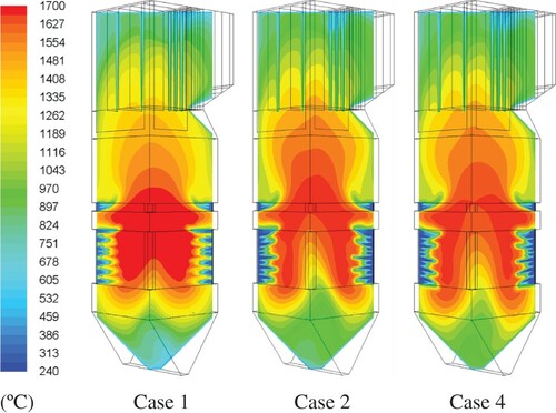
Figure 6 presents the heat flux distributions of the furnace wall for Cases 1, 2 and 4. It is shown that, because of the reduced flame temperature, the wall heat flux in the coal switching cases (Cases 2 and 4) is considerably lower than that of Case 1. In Case 4, because tilting the burner down extends the high-temperature flame deeper into the furnace space, its wall heat flux appears higher than that of Case 2.

Figure 6. Heat flux distributions on the furnace right wall.

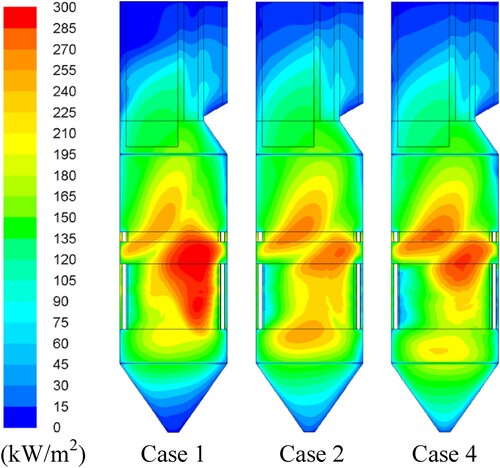
Figure 7 shows the calculated heat transfer results for the different cases with the corresponding data summarized in Table 6. It can be seen that the total heat absorption of the furnace wall is reduced from 347.6 MW for Case 1 to 337.7 MW for Case 2. Consequently, in Case 2 the heat absorption by the downstream superheaters is increased. In Case 3, 3.33 kg/s cooling sprays are applied to each of the two spray attemperators. The spray flows reduce the steam temperatures in the DPSH, the PLSH and the SSH and, hence, the temperature differences between the gas and steam flows in these superheaters are increased. Thus, the heat transfer to the DPSH, the PLSH and the SSH increase slightly compared to Case 2. Since the DPSH, the PLSH and the SSH are located downstream of the furnace exit, the heat transfer in the main furnace is affected little. Thus, Cases 2 and 3 have very close furnace wall heat absorption. However, the increased heat transfer to the DPSH, the PLSH and the SSH reduces the overall gas temperature downstream of these superheaters in the convection pass. As a result, the heat absorption of the heat exchangers in the convection pass (e.g. the PSHs and the ECON) are reduced compared to Case 2. As discussed before, the heat transfer calculations of all boiler heating surfaces are coupled through the interaction of gas and steam temperatures. The results here clearly demonstrate that the coupled heat transfer model can effectively capture this coupled behavior. Case 4 is the burner tilt case. As seen in Figure 7 and Table 6, the wall heat absorption of Case 4 is increased and, consequently, the heat transfer distributions of Cases 1 and 4 are similar. The economizer is located at the outlet of the boiler. Any changes occurring in the boiler will be compensated by the heat exchangers upstream of the economizer. Thus, the heat absorption of the economizer varies very little for different cases.

Figure 7. Predicted heat transfer distributions for different cases.

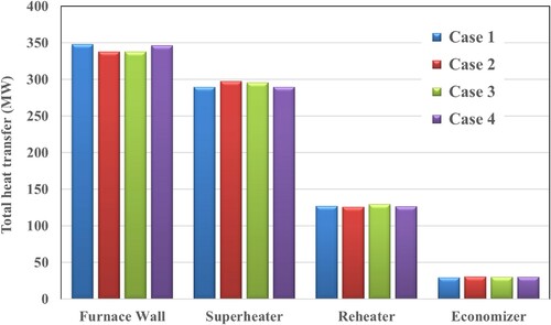
Table 6. Heat absorption of each boiler heating surface.

	Heat absorption, MW
Heating surfaces	Case 1	Case 2	Case 3	Case 4
ECON	28.84	30.08	29.69	29.64
WALL	347.61	337.67	337.46	346.13
ROOF	20.47	21.69	20.93	19.84
PSH1	8.84	9.52	9.16	9.24
PSH2	16.83	17.98	17.40	17.33
PSH3	24.94	26.38	25.63	25.53
PSH4	36.59	38.25	37.09	37.39
PSH5	39.70	40.88	39.76	40.16
DPSH	51.70	53.12	53.44	50.28
PLSH	59.77	59.57	60.22	59.19
SSH	30.68	30.03	31.52	30.69
WRH	33.95	35.37	35.92	33.24
CRH	58.44	57.16	58.75	58.38
HRH	34.17	33.12	34.49	34.24

Figure 8 shows the steam temperature variations along the steam cycle. Table 7 summarizes the predicted water/steam flow rates and steam temperatures at the outlets of each boiler heating surface and HP turbine for the four cases. It is seen that the feedwater flow rates of Cases 2 and 3 are lower than that of Case 1 due to the reduced evaporative heat absorption of the furnace wall. The reduced steam flow along with the increased SH heat absorption leads to the considerable increase of the final SH steam temperature of Case 2 by 17.3°C. As seen in Figure 8, the increased SH steam temperature leads to increased RH steam temperature at the inlet of reheaters, which subsequently leads to the increase of the final RH temperature by 23.0°C. The increases of the final SH and RH steam temperatures by ∼20.0°C are rather remarkable. Maintaining the steam temperatures stable at the boiler’s designated values ∼540°C is the most crucial part of boiler operation. Lower steam temperatures directly reduce the boiler’s thermal efficiency. Higher steam temperatures are generally strictly prohibited by the plant operators since this would cause thermal fatigue of the steam turbines and piping system. If the steam temperatures cannot be reduced effectively through operational adjustments, the boilers have to de-rate to protect the steam turbines and piping. Either case will severely hurt the thermal performance of the boiler and cause significant economic losses of the power plants. In order to examine if the increased steam temperatures can be recovered, in Case 3, 3.33 kg/s of cooling sprays are applied through the attemperators before the DPSH and the SSH, respectively. As shown in Figure 8, the cooling spray reduces the steam temperatures at the inlets of the DPSH and the SSH and, consequently, brings the final SH and RH steam temperatures back to ∼540°C. Since 3.33 kg/s spray is well within the maximum capacity of the spray attemperators (∼16.7 kg/s), the predicted results indicate that the boiler can still maintain its original steam temperatures after coal switching. Case 4 is another boiler operational adjustment attempting to recover the final SH and RH steam temperatures by adjusting the injection direction of coal and air streams. As seen in Figures 7 and 8, the boiler heat transfer distribution and the SH and RH steam temperatures along the steam cycle of Case 4 are very close to those of Case 1. Since the maximum allowable burner tilt angles are ±30°, the predicted results indicate that burner setting adjustment is another effective way to maintain the boiler steam temperatures after coal switching. The major reasons for this boiler to be able to maintain its steam temperatures after coal switching is that the baseline case (Case 1) did not experience overheated steam and no spray attemperation was applied to control the steam temperatures. This is, however, not the case if the boiler has already maximized its spray attemperation.

Figure 8. Predicted steam temperature variations along the steam cycle.

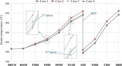
Table 7. The water/steam flow rates and steam temperatures at the outlets of heating surfaces.

	Flow rate, t/h
	Case 1	Case 2	Case 3	Case 4
Feedwater	1065.0	1040.1	1038.4	1062.8
Spray	0.0	0.0	24.0	0.0
SH steam	1065.0	1040.1	1062.4	1062.8
RH steam	965.0	942.4	962.6	962.9
Outlet	Steam temperature, °C
ECON	281.0	282.3	282.1	281.6
WALL	365.8	365.8	365.8	365.8
ROOF	367.1	367.4	367.3	367.0
PSH1	367.5	367.9	367.8	367.5
PSH2	369.5	370.4	370.0	369.5
PSH3	375.0	377.0	376.2	375.2
PSH4	388.3	392.7	390.9	389.1
PSH5	410.0	417.5	414.2	411.5
DPSH	450.0	462.4	451.8	450.8
PLSH	509.0	525.3	512.6	509.4
SSH	543.0	560.3	538.7	543.5
HPT	345.8	360.8	342.2	346.3
WRH	396.0	415.5	395.1	395.4
CRH	488.0	508.4	487.7	487.4
HRH	540.0	563.0	543.3	542.6

Note: Bold values: The outlet steam temperatures of SSH and HRH mean the final SH and RH steam temperatures generated by the boiler,respectively. They are the most essential operating prameters of a boiler.

6. Conclusions

A coupled boiler heat transfer model that integrates the boiler’s fire side CFD solution with the boiler’s steam temperatures has been developed in this study. This model is capable of predicting the steam temperature variations along the entire steam cycle without resort to a second process model. It is designed to provide efficient computational solutions to practical boiler problems wherein the change of boiler steam temperatures subject to different boiler design and operation conditions are of major concern.

This coupled heat transfer model was applied to a 320 MW subcritical boiler to evaluate the impacts of coal switching and boiler operation conditions on the boiler’s heat transfer distribution and steam temperatures. The results show that the evaporation heat absorption of the furnace water wall is reduced and, consequently, the heat absorption by the downstream superheaters and reheaters is increased after switching to a coal with reduced heating value. This results in a significant increase of the final SH and RH steam temperatures. The increase of steam temperatures, however, can be recovered through boiler operational adjustments, such as attemperation spray and burner tilt. The simulation results illustrate that the coupled model can capture the complex coupled heat transfer behavior between the fire and steam sides of boiler effectively, and serve as an efficient predictive tool for practical boiler applications.

Nomenclature

$A_{\text{c}}$	=	Pre-exponential factor for the char surface reaction model, kg/(m2·s·atm)
$A_{\text{v}}$	=	Pre-exponential factor for the coal devolatilization model, s−1
Ec	=	Activation energy for the char surface reaction model, J/mole
Ev	=	Activation energy for the coal devolatilization model, J/mole
$h_{\text{econ}}^{\text{out}}$	=	Specific enthalpy of water out of the economizer, kJ/kg
$h_{\text{roof}}^{\text{out}}$	=	Specific enthalpy of steam out of the ROOF superheater, kJ/kg
$h_{\text{hp}}^{\text{out}}$	=	Specific enthalpy of steam out of the high-pressure turbine, kJ/kg
$h_{\text{hp}}^{\text{out},s}$	=	Specific enthalpy of steam out of the high-pressure turbine for an isentropic process, kJ/kg
$h_{\text{sat},v}$	=	Specific enthalpy of saturated steam, kJ/kg
$h_{\text{ssh}}^{\text{out}}$	=	Specific enthalpy of steam out of the final superheater, kJ/kg
$h_{\text{wrh}}^{\text{in}}$	=	Specific enthalpy of steam at the inlet of the wall reheater, kJ/kg
$h_{\text{wrh}}^{\text{out}}$	=	Specific enthalpy of steam out of the wall reheater, kJ/kg
${\mathcal{H}}_{\text{ext}}$	=	Wall heat transfer coefficient, W/(m2·K)
${\mathcal{H}}_f$	=	Gas side heat transfer coefficient of convective heat exchangers, W/(m2·K)
${\dot{m}}_{\text{feed}}$	=	Flow rate of boiler feedwater, kg/s
${\dot{m}}_{\text{rh}}$	=	Flow rate of reheat steam, kg/s
${\dot{m}}_{\text{sh}}$	=	Flow rate of superheat steam, kg/s
${\dot{m}}_{\text{spray}}$	=	Flow rate of attemperation spray, kg/s
q	=	Heat flux of furnace wall, W/m2
qconv	=	Heat absorption of convective heat exchangers per unit volume, W/m3
$Q_{\text{psh}1}$	=	Heat absorption of the PSH1 superheater, W
$Q_{\text{roof}}$	=	Heat absorption of the ROOF superheater, W
$Q_{\text{wall}}^{DCS}$	=	Heat absorption of the furnace wall estimated from the boiler steam parameters, W
$Q_{\text{wall}}$	=	Heat absorption of the furnace wall calculated from the CFD solution, W
$Q_{\text{wrh}}$	=	Heat absorption of the wall reheater, W
Sconv	=	Outer surface area of convective heat exchangers per unit volume, m−1
$T_{\text{ssh}}^{\text{out}}$	=	Steam temperature out of the final superheater, °C
$T_{\text{hrh}}^{\text{out}}$	=	Steam temperature out of the final reheater, °C
Tf	=	Flue gas temperature, °C
Ts	=	Water/steam temperature in boiler heating surface tubes, °C
Tsat,v	=	Saturation temperature of steam, °C
Tw	=	Furnace wall ash layer surface temperature, °C

Greek characters

$\psi$	=	Thermal effective factor of convective heat exchangers
${\eta }_{\text{hp}}$	=	Isentropic efficiency of a high-pressure turbine

Disclosure statement

No potential conflict of interest was reported by the authors.

References

- Abadi, A. M. E., Sadi, M., Farzaneh-Gord, M., Ahmadi, M. H., Kumar, R., & Chau, K. W. (2020). A numerical and experimental study on the energy efficiency of a regenerative Heat and Mass Exchanger utilizing the counter-flow Maisotsenko cycle. Engineering Applications of Computational Fluid Mechanics, 14(1), 1–12. https://doi.org/https://doi.org/10.1080/19942060.2019.1617193
- Adamczyk, W. P., Werle, S., & Ryfa, A. (2014). Application of the computational method for predicting NOx reduction within large scale coal-fired boiler. Applied Thermal Engineering, 73(1), 343–350. https://doi.org/https://doi.org/10.1016/j.applthermaleng.2014.07.045
- Ansys CFX: Computational Fluid Dynamics (CFD) Software Program Solutions. https://www.ansys.com/products/fluids/ansys-cfx
- ANSYS Fluent: Fluid Simulation Software. https://www.ansys.com/products/fluids/ansys-fluent
- APROS Advanced Process Simulation Software. https://www.fortum.com/products-and-services
- Backreedy, R. I., Habib, R., Jones, J. M., Pourkashanian, M., & Williams, A. (1999). An extended coal combustion model. Fuel, 78(14), 1745–1754. https://doi.org/https://doi.org/10.1016/S0016-2361(99)00123-4
- Backreedy, R. I., Jones, J. M., Ma, L., Pourkashanian, M., Williams, A., Arenillas, A., Arias, B., Pis, J. J., & Rubiera, F. (2005). Prediction of unburned carbon and NOx in a tangentially fired power station using single coals and blends. Fuel, 84(17), 2196–2203. https://doi.org/https://doi.org/10.1016/j.fuel.2005.05.022
- Badzioch, S., & Hawksley, P. G. W. (1970). Kinetics of thermal decomposition of pulverized coal particles. Industrial & Engineering Chemistry Process Design and Development, 9(4), 521–530. https://doi.org/https://doi.org/10.1021/i260036a005
- Baum, M. M., & Street, P. J. (1971). Predicting the combustion behaviour of coal particles. Combustion Science and Technology, 3(5), 231–243. https://doi.org/https://doi.org/10.1080/00102207108952290
- Boyd, R. K., & Kent, J. H. (1988). Three-dimensional furnace computer modelling. Symposium (International) on Combustion, 21(1), 265–274. https://doi.org/https://doi.org/10.1016/S0082-0784(88)80254-6
- BP Statistical Review of World Energy. (2019). www.bp.com/statisticalreview
- Che, D. F. (2008). Boiler - theory, design and operation. Xi'an Jiaotong University Press.
- Chen, T., Zhang, Y. J., Liao, M. R., & Wang, W. Z. (2019). Coupled modeling of combustion and hydrodynamics for a coal-fired supercritical boiler. Fuel, 240, 49–56. https://doi.org/https://doi.org/10.1016/j.fuel.2018.11.008
- COMSOL – Software for Multiphase Simulation. www.comsol.com
- Diez, L. I., Cortes, C., & Pallares, J. (2008). Numerical investigation of NOx emissions from a tangentially-fired utility boiler under conventional and overfire air operation. Fuel, 87(7), 1259–1269. https://doi.org/https://doi.org/10.1016/j.fuel.2007.07.025
- Edge, P. J., Heggs, P. J., Pourkashanian, M., & Stephenson, P. L. (2013). Integrated fluid dynamics-process modelling of a coal-fired power plant with carbon capture. Applied Thermal Engineering, 60(1-2), 456–464. https://doi.org/https://doi.org/10.1016/j.applthermaleng.2012.08.031
- Edge, P. J., Heggs, P. J., Pourkashanian, M., Stephenson, P. L., & Williams, A. (2012). A reduced order full plant model for oxyfuel combustion. Fuel, 101, 234–243. https://doi.org/https://doi.org/10.1016/j.fuel.2011.05.005
- Edge, P. J., Heggs, P. J., Pourkashanian, M., & Williams, A. (2011). An integrated computational fluid dynamics-process model of natural circulation steam generation in a coal-fired power plant. Computers & Chemical Engineering, 35(12), 2618–2631. https://doi.org/https://doi.org/10.1016/j.compchemeng.2011.04.003
- Flownex Simulation Environment. https://flownex.com/
- Gandhi, M. B., Vuthaluru, R., Vuthaluru, H., French, D., & Shah, K. (2012). CFD based prediction of erosion rate in large scale wall-fired boiler. Applied Thermal Engineering, 42, 90–100. https://doi.org/https://doi.org/10.1016/j.applthermaleng.2012.03.015
- gRPOMS Process Engineering Software. https://www.psenterprise.com/products/gproms
- Hu, Y. K., Li, H. L., & Yan, J. Y. (2014). Numerical investigation of heat transfer characteristics in utility boilers of oxy-coal combustion. Applied Energy, 130, 543–551. https://doi.org/https://doi.org/10.1016/j.apenergy.2014.03.038
- Laubscher, R., & Rousseau, P. (2019a). CFD study of pulverized coal-fired boiler evaporator and radiant superheaters at varying loads. Applied Thermal Engineering, 160, 114057. https://doi.org/https://doi.org/10.1016/j.applthermaleng.2019.114057
- Laubscher, R., & Rousseau, P. (2019b). Numerical investigation into the effect of burner swirl direction on furnace and superheater heat absorption for a 620 MWe opposing wall-fired pulverized coal boiler. International Journal of Heat and Mass Transfer, 137, 506–522. https://doi.org/https://doi.org/10.1016/j.ijheatmasstransfer.2019.03.150
- Laubscher, R., & Rousseau, P. (2020). Numerical investigation on the impact of variable particle radiation properties on the heat transfer in high ash pulverized coal boiler through co-simulation. Energy, 195, 117006. https://doi.org/https://doi.org/10.1016/j.energy.2020.117006
- Lee, F. C. C., & Lockwood, F. C. (1999). Modelling ash deposition in pulverized coal-fired applications. Progress in Energy and Combustion Science, 25(2), 117–132. https://doi.org/https://doi.org/10.1016/S0360-1285(98)00008-2
- Liu, H., Wang, Y. K., Zhang, W., Wang, H., Deng, L., & Che, D. F. (2019). Coupled modeling of combustion and hydrodynamics for a 1000MW double-reheat tower-type boiler. Fuel, 255, 115722. https://doi.org/https://doi.org/10.1016/j.fuel.2019.115722
- Liu, H., Zhang, W., Wang, H., Zhang, Y. H., Deng, L., & Che, D. F. (2020). Coupled combustion and hydrodynamics simulation of a 1000MW double-reheat boiler with different FGR positions. Fuel, 261, 116427. https://doi.org/https://doi.org/10.1016/j.fuel.2019.116427
- Lockwood, F. C., Salooja, A. P., & Syed, S. A. (1980). A prediction method for coal-fired furnaces. Combustion and Flame, 38, 1–15. https://doi.org/https://doi.org/10.1016/0010-2180(80)90033-4
- Magnussen, B. F., & Hjertager, B. H. (1977). On mathematical modelling of turbulent combustion with special emphasis on soot formation and combustion. Symposium (International) on Combustion, 16(1), 719–729. https://doi.org/https://doi.org/10.1016/S0082-0784(77)80366-4
- MATLAB - MathWorks. https://www.mathworks.com/products/matlab.html
- Mitchell, R. E., Hurt, R. H., Baxter, L. L., & Hardesty, D. R. (1992). Compilation of Sandia coal char combustion data and kinetic analyses, milestone report. SAND 92-8208.
- Niksa, S. (1995). Predicting the devolatilization behavior of any coal from its ultimate analysis. Combustion and Flame, 100(3), 384–394. https://doi.org/https://doi.org/10.1016/0010-2180(94)00060-6
- Park, H. Y., Faulkner, M., Turrell, M. D., Stopford, P. J., & Kang, D. S. (2010). Coupled fluid dynamics and whole plant simulation of coal combustion in a tangentially-fired boiler. Fuel, 89(8), 2001–2010. https://doi.org/https://doi.org/10.1016/j.fuel.2010.01.036
- Park, S., Kim, J. A., Ryu, C., Chae, T., Yang, W., Kim, Y. J., Park, H.-Y., & Lim, H. C. (2013). Combustion and heat transfer characteristics of oxy-coal combustion in a 100 MWe front-wall-fired furnace. Fuel, 106, 718–729. https://doi.org/https://doi.org/10.1016/j.fuel.2012.11.001
- Ramezanizadeh, M., Nazari, M. A., Ahmadi, M. H., & Chau, K. W. (2019). Experimental and numerical analysis of a nanofluidic thermosyphon heat exchanger. Engineering Applications of Computational Fluid Mechanics, 13(1), 40–47. https://doi.org/https://doi.org/10.1080/19942060.2018.1518272
- Rousseau, P., & Laubscher, R. (2020). Analysis of the impact of coal quality on the heat transfer distribution in a high-ash pulverized coal boiler using co-simulation. Energy, 198, 117343. https://doi.org/https://doi.org/10.1016/j.energy.2020.117343
- Schuhbauer, C., Angerer, M., Spliethoff, H., Kluger, F., & Tschaffon, H. (2014). Coupled simulation of a tangentially hard coal fired 700°C boiler. Fuel, 122, 149–163. https://doi.org/https://doi.org/10.1016/j.fuel.2014.01.032
- Spitz, N., Saveliev, R., Perelman, M., Korytni, E., Chudnovsky, B., Talanker, A., & Bar-Ziv, E. (2008). Firing a sub-bituminous coal in pulverized coal boilers configured for bituminous coals. Fuel, 87(8-9), 1534–1542. https://doi.org/https://doi.org/10.1016/j.fuel.2007.08.020
- Tan, P., Fang, Q. Y., Zhao, S. N., Yin, C. E., Zhang, C., Zhao, H. B., & Chen, G. (2018). Causes and mitigation of gas temperature deviation in tangentially fired tower-type boilers. Applied Thermal Engineering, 139, 135–143. https://doi.org/https://doi.org/10.1016/j.applthermaleng.2018.04.131
- Tan, P., Tian, D. F., Fang, Q. Y., Ma, L., Zhang, C., Chen, G., Zhong, L., & Zhang, H. G. (2017). Effects of burner tilt angle on the combustion and NOx emission characteristics of a 700 MWe deep-air-staged tangentially pulverized-coal-fired boiler. Fuel, 196, 314–324. https://doi.org/https://doi.org/10.1016/j.fuel.2017.02.009
- Truelove, J. S. (1984). The modelling of flow and combustion in swirled, pulverized-coal burners. Symposium (International) on Combustion, 20(1), 523–530. https://doi.org/https://doi.org/10.1016/S0082-0784(85)80541-5
- Wang, H. Y., Zhang, C. Q., & Liu, X. (2020). Heat transfer calculation methods in three-dimensional CFD model for pulverized coal-fired boilers. Applied Thermal Engineering, 166, 114633. https://doi.org/https://doi.org/10.1016/j.applthermaleng.2019.114633
- Weber, R., Mancini, M., Schaffel-Mancini, N., & Kupka, T. (2013). On predicting the ash behaviour using Computational Fluid Dynamics. Fuel Processing Technology, 105, 113–128. https://doi.org/https://doi.org/10.1016/j.fuproc.2011.09.008
- Yang, W. J., You, R. Z., Wang, Z. H., Zhang, H. T., Zhou, Z. J., Zhou, J. H., Guan, J., & Qiu, L. C. (2017). Effects of near-wall Air application in a pulverized-coal 300 MWe utility boiler on combustion and corrosive gases. Energy & Fuels, 31(9), 10075–10081. https://doi.org/https://doi.org/10.1021/acs.energyfuels.7b01476
- Yin, C., Caillat, S., Harion, J. L., Baudoin, B., & Perez, E. (2002). Investigation of the flow, combustion, heat-transfer and emissions from a 609 MW utility tangentially fired pulverized-coal boiler. Fuel, 81(8), 997–1006. https://doi.org/https://doi.org/10.1016/S0016-2361(02)00004-2
- Zhang, X. H., Zhou, J., Sun, S. Z., Sun, R., & Qin, M. (2015). Numerical investigation of low NOx combustion strategies in tangentially-fired coal boilers. Fuel, 142, 215–221. https://doi.org/https://doi.org/10.1016/j.fuel.2014.11.026