
 ?Mathematical formulae have been encoded as MathML and are displayed in this HTML version using MathJax in order to improve their display. Uncheck the box to turn MathJax off. This feature requires Javascript. Click on a formula to zoom.
Abstract
Vortex is the dominant flow structure in hydro-energy machinery, and its swirling features are mainly determined by the rigid rotation part of vorticity. In this study, the rigid vorticity transport equation is proposed based on the vorticity decomposition. The vortex spatial evolution is described by the stretching term RST, the dilatation term RDT, the Lamb term RCT and the viscous term RVT. The shape change of a vortex tube is mainly affected by RST and RDT, while vortex production and dissipation are mainly reflected by RCT and RVT. Compared with the traditional vorticity transport equation, this new theoretical tool can distinguish between rigid rotation and shearing motion of local fluids, and it can better reveal the intuitive evolution characteristics of vortical structures. Two cases with clear engineering demands are analysed by using the transport equation, and the results show that it can provide a practical method for the analysis and control of vortical flows in hydro-energy machinery.
1. Introduction
Hydro-energy machinery (e.g. hydro turbines and water pumps) plays a significant role in energy engineering. There are many important vortical structures in hydro-energy machinery, such as the inter-blade vortex (Yamamoto et al., Citation2017), Kármán vortex (Nennemann & Monette, Citation2018), tip leakage vortex (Dreyer et al., Citation2014) and helical vortex rope (Pasche et al., Citation2017), etc. The evolution of vortical structures in hydro-energy machinery can cause a lot of unsteady flow phenomena, such as rotating stall (Zhang et al., Citation2017), vortex cavitation (Wang et al., Citation2018), severe pressure fluctuation and vibration (Zhao et al., Citation2017), seriously affecting the safe operations. It is an important task for turbulent flow analysis in hydro-energy machinery to effectively identify a vortex and understand its intuitive evolution characteristics.
The classical theory of vortex dynamics was developed on the basis of vorticity (Truesdell, Citation1954), which is an important physical quantity originating from the Cauchy-Stokes decomposition of the velocity gradient tensor (Wu et al., Citation2006) and has a rigorous mathematical definition (ω=▿×V). However, according to the studies of Robinson, Kline, and Spalart (Citation1989) and Jeong and Hussain (Citation1995), the association between the regions of strong vorticity and actual vortices seems to be rather weak, and vorticity does not identify a vortex in shear flows especially if the background shear is comparable to the vorticity magnitude within the vortex. This suggests that vorticity is not necessarily equivalent to vortex. In fact, the idea of vorticity decomposition was studied early on by Astarita (Citation1979), Lindgren (Citation1980), Jiang (Citation1999) and Wedgewood (Citation1999). It indicates that total vorticity ω can be decomposed into the rigid vorticity ωR and the deformational vorticity ωS. The former induces the rigid rotation motions of a fluid element, while the latter induces the pure shearing motions. Obviously, ωR can be used to mark the vortex region (identification and visualization) which is characterized by rigid rotation, while ωS can reflect the shearing effect (rubbing emphasized by Prof. Shijia Lu) which induces the vortical motions. To distinguish between rigid rotation and pure shearing in total vorticity, the residual vorticity was proposed by Kolář (Citation2007), and the precise mathematical expression of the rigid vorticity ωR was given by Liu et al. (Citation2018, Citation2019), which is referred to as Liutex (originally known as Rortex). Moreover, according to the studies of Das and Girimaji (Citation2020b), it is found that low-pressure regions are strongly associated with rigid rotation motions, while pure shearing is associated with nearly zero pressure fluctuations. Vortex-induced pressure fluctuation and vibration are important topics in system stability studies of hydro-energy machinery. To address this engineering demand, it is reasonable and necessary to introduce this vorticity decomposition scheme.
Vorticity is the only criterion for which a transport equation is well known and the only possible choice to study the vortex dynamics in turbulence (Cuissa & Steiner, Citation2020). However, due to the fact that total vorticity ω cannot distinguish between rigid rotation ωR and pure shearing ωS, this traditional tool cannot well extract the intuitive vortex evolution characteristics, which makes it unsuitable for effective control of vortical structures in hydro-energy machinery. According to the previous studies of the authors (Wang et al., Citation2020, Citation2021b), the rigid vorticity ωR provides a new insight into the physics of turbulent vortices and has been successfully used in Eulerian vortex identification and visualization, but its transport equation is yet to be developed. Accordingly, the objective of this paper is to provide a practical method for more effective analysis and control of vortical flows in hydro-energy machinery by using this new physical quantity.
The article structure is arranged as follows: In Section 2, the vorticity decomposition scheme is introduced and the rigid vorticity transport equation is proposed. In Section 3 and Section 4, two cases with clear engineering demands, trailing edge modification of a hydrofoil and inverse design of a centrifugal pump impeller, are analysed by using this new theoretical tool. In Section 5, the conclusions are given.
2. Vorticity decomposition scheme
2.1 Vorticity binary decomposition
According to the idea of vorticity binary decomposition, total vorticity ω can be further decomposed into the rigid vorticity ωR and the deformational vorticity ωS. This relationship is expressed as (Liu et al., Citation2018)
(1)
(1)
where the rigid vorticity ωR induces rigid rotation motions of local fluids. The direction and magnitude of ωR are firstly determined. Since only stretching motions (normal strain) exist in the rigid rotation axis direction r (▿V·r=λ·r), the direction of ωR should be aligned with an eigenvector of the velocity gradient tensor ▿V. Accordingly, combined with the studies of Chong et al. (Citation1990) and Zhou et al. (Citation1999), if the velocity gradient tensor ▿V has one real and two complex conjugate eigenvalues, the real eigenvector corresponding to the real eigenvalue serves as the rigid rotation axis. Moreover, for a velocity gradient tensor ▿Vxyz in an ordinary reference frame xyz, two rotation matrices can be employed in the transformation to a new reference frame XYZ (Tian et al., Citation2018), in which the local fluid rotation axis is aligned with the Z-axis. The orthogonal coordinate system with the direction vector r as its Z-axis is also known as the basic reference frame (BRF), and the corresponding velocity gradient tensor ▿VXYZ in the BRF is expressed as
(2)
(2)
where O is the first rotation matrix, P is the second rotation matrix, λcr and λr contribute to the normal strain of local fluid motions, and s, ξ and η contribute to pure shearing. In particular, φ is the angular velocity of rigid rotation, and the magnitude of ωR is 2φ. According to Equation (2), an additive decomposition of the velocity gradient tensor (rigid rotation + pure shearing + irrotational strain) can be realized based on the rigid rotation rate tensor [R] (Gao & Liu, Citation2019), which is given by
(3)
(3)
This triple decomposition of ▿V emphasizes the rigid rotation component in an explicit manner. Moreover, to provide a simple algorithm for ωR, an explicit expression was derived by Wang et al. (Citation2019), which is given by
(4)
(4)
where [ε] is the Levi-Civita permutation tensor, and λci was referred to as swirling strength (Zhou et al., Citation1999) and is the imaginary part of the complex conjugate eigenvalues of ▿V. Rigid vorticity is a mathematically rigorous tool suitable for vortex identification and visualization (Kolář & Šístek Citation2020; Zhan et al., Citation2019, Citation2020), and its transport can reflect the vortex evolution process. According to the vorticity ω and its rotation part ωR, the shearing part ωS can also be determined (ωS=ω-ωR).
2.2 The effects of deformational vorticity on rigid vorticity
Although the two components of total vorticity ω can be calculated accurately, the relationship between them, especially the effects of deformational vorticity ωS on rigid vorticity ωR, is still lacking in a more intuitive explanation. Interestingly, according to the group theory, the natural exponent of a skew symmetric matrix is an SO(3) orthogonal rotation matrix, the three column vectors of which can directly form an orthogonal coordinate system consolidated in a local objective. This property makes it easy to further study the relationship between the two components from a geometric perspective.
According to Equation (3), the rigid rotation rate tensor [R] is an antisymmetric quantity decomposed from the skew symmetric part of the velocity gradient tensor ▿V (rotation rate tensor [Ω]), and thus the two SO(3) orthogonal rotation matrices generated by [R] and [Ω] are e[R] and e[Ω], respectively. In particular, the latter (e[Ω]) is also known as the tensor [Q] defined by Sun (Citation2019), the expansion of which is expressed as
(5)
(5)
and the skew symmetric part of velocity gradient tensor ▿VXYZ in the BRF is given by
(6)
(6)
where ω1, ω2 and ω3 are the components of the vorticity-based angular velocity ω. Accordingly, the tensor [Q] in Equation (5) can be expanded as
(7)
(7)
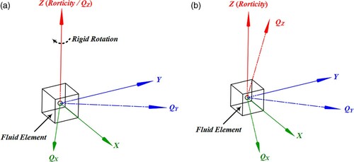
where δij is the Kronecker delta, and εijk is the Levi-Civita symbol. Taking the XOY plane of BRF as the basic reference surface, ω1 (∂VW/2∂Y) and ω2 (-∂VW/2∂X) reflect the effects of normal shearing, and ω3 reflects the effects of rigid rotation and tangential shearing.
(8)
(8)
As shown in Figure (a), if there are no shearing effects, a degenerate form of [Q] is e[R], which is given by Equation (8) and represents the rolling trend around the Z-axis (or the rigid rotation axis), which is a typical form of Euler attitude. As shown in Figure (b), if there exist both normal and tangential shearing effects, the other two forms of attitude trends, yawing and pitching, will also appear. For a fluid element, a general expression between the e[Ω] (vorticity) and e[R] (rigid vorticity) can be expressed as ABC[Q] = e[R] by using three Euler transformation matrices to eliminate the pure shearing effects, and the details are given in the Appendix, which presents the motion trend of a fluid element under the actions of rigid rotation (φ) and pure shearing (s, ξ, and η). Obviously, it is the complex shearing effects (s, ξ, and η) that change the simple feature of rigid rotation motion. Besides, the divergence of vorticity is given by
(9)
(9) which indicates that the source intensity of deformational vorticity directly affects the birth-and-death of rigid vorticity. Accordingly, the rigid rotation motion, a special existence form of local fluids, is controlled by the shearing motion that definitely exists in the general flows. This may be the reason why the shearing part is usually dominant in total vorticity (Das & Girimaji, Citation2020a).
Figure 1. Geometric description of the two orthogonal rotation tensors. (a) Degenerate form (rigid rotation trend). (b) General form (synthetic attitude trend).
2.3 Rigid vorticity transport equation
Since ωR originates from vorticity ω, the classical vorticity transport equation is exactly an important theoretical basis. For the three-dimensional viscous flows, the transport equation of vorticity ω (Friedman equation) is expressed as (Wu et al., Citation2006)
(10)
(10)
where υ is the kinematic viscosity, f is the body force, ρ is the density, and p is the static pressure. Under the cavitation-free condition, for the turbulent flows in hydro-energy machinery, the conditions of incompressible flow (▿·V=0), conservative body force (▿×f=0) and barotropic fluid (-▿×(▿p/ρ) = 0) are usually ensured. Accordingly, a degenerate form of the general vorticity transport equation is given by
(11)
(11)
which shows that the existing vorticity is convected, stretched, turned, and diffused (kinematics characteristics). Combined with the binary decomposition of vorticity, Equation (11) can be equivalently transformed into a novel form with rigid vorticity ωR as the transport quantity, which is expressed as
(12)
(12)
Obviously, the transport of rigid vorticity is inseparable from the induction effects of pure shearing motions, which is consistent with the analysis in subsection 2.2. In engineering applications, we first focus on the evolution of vortical structures in the spatial dimension (convective derivative), and thus Equation (12) can be further expressed as
(13)
(13)
where LR=ωR×V is referred to as the pseudo Lamb vector in this study, the first right-hand member is referred to as the rigid vorticity stretching term (RST), the second right-hand member is referred to as the rigid vorticity dilatation term (RDT), the third right-hand member is referred to as the curl term of the pseudo Lamb vector (RCT), and the last right-hand member is referred to as the viscous term (RVT).
Theoretically, RST can be used to represent the normal strain (tension or compression) of the vortex core line (note that ωR·▿V=λrωR·r). RDT is determined by the divergence of rigid vorticity and the local induced velocity, and its direction is parallel to the local velocity vector V, which indicates that RDT can be used to represent the tangential strain (torsion or bending) of the vortex tube in the convection process. RCT contains the effects of shearing motion and local acceleration, and it can be used to reflect the intensity change of rigid vorticity according to the Biot-Savart law. RVT can be used to represent the diffusion and dissipation of rigid vorticity caused by the viscous effects, and it can be transformed into (Reynolds averaging operation) to reflect the turbulent effects. The shape change of a vortex tube is mainly affected by RST and RDT, and the vortex production and dissipation are mainly reflected by RCT and RVT.
In the impellers of hydro turbine and water pump, the Coriolis effect 2ωi·▿V appears as a natural term, and ωi is the angular velocity of the impeller. This term is referred to as ROT and has important effects on the vortex evolution in the rotating systems. Overall, the rigid vorticity transport equation is an equivalent form of the classical vorticity transport equation, which emphasizes the transport of its rigid rotation part. It can become a new theoretical tool for the vortex spatial evolution analysis in hydro-energy machinery.
3. Application case I: trailing edge modification of a hydrofoil
3.1 Engineering background and application objective
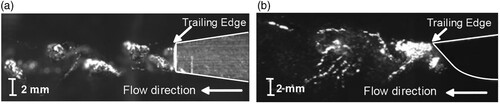
Hydrofoil is the basic unit of impeller and guide-vane domains in hydro-energy machinery. Wake vortex shedding of a hydrofoil can induce great vibration and may even cause severe fatigue damage (Dörfler et al., Citation2013; Trivedi, Citation2017). A good trailing edge modification method can effectively reduce the vibration and noise induced by wake vortex shedding (Ausoni, Citation2009; Zobeiri et al., Citation2012). As shown in Figure , Donaldson trailing edge (DTE) is a typical modification strategy, which is characterized by a progressive smooth change in the slope of the hydrofoil trailing edge (Donaldson, Citation1956). Compared with the blunt trailing edge (BTE), the hydrodynamic damping is increased, and the added mass is decreased for the hydrofoil with DTE (Yao et al., Citation2014; Zeng et al., Citation2019), which has an important contribution to the reduction of vibration. The engineering value of trailing edge modification has been recognized, while the flow mechanism behind it is yet to be clarified (Hu et al., Citation2020). Accordingly, the first application case is discussed based on the engineering demand of providing the direct reason for the increase in hydrodynamic damping of the DTE hydrofoil.
Figure 2. Experimental observation of wake vortices (Zobeiri, Citation2012). (a) BTE hydrofoil. (b) DTE hydrofoil.
3.2 V&V of numerical simulation scheme
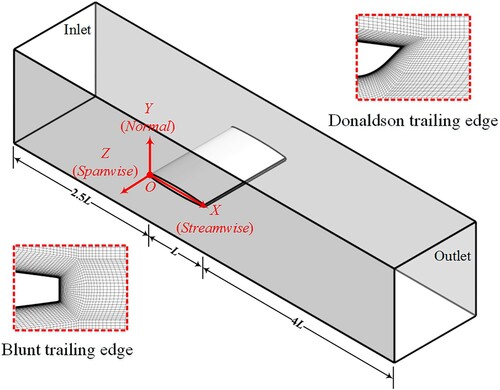
As shown in Figure , the computational domain of this flow case is determined according to the experiment conducted in the EPFL (Ausoni, Citation2009; Zobeiri, Citation2012). A NACA0009 hydrofoil is used to induce the wake vortex shedding. The length of water tank is 750 mm, and the cross section of it is square (150 mm×150 mm). The attack angle is α=0° and the chord length is L=100 mm. Reynolds number determined by the free-stream velocity V0 = 20m/s and the chord length L is approximately Re=2×10⁶. The trailing edge thickness the BTE is h=3.22mm, and the Donaldson modification is performed based on this BTE, which consists of a 45° oblique tangent line and a cubic polynomial curve (Zobeiri, Citation2012).
Figure 3. Computational domain of flow around a hydrofoil.
ANSYS CFX are used for numerical simulations of the flow fields, and the classical SST k-ω turbulence model with the γ-Reθt transition model is employed. There are many novel CFD models for the foils (Ghalandari et al., Citation2019; Salih et al., Citation2019), but this classical modelling scheme is popular for turbulent flow computations in hydro-energy machinery, and its reliability has been demonstrated in the previous studies of the authors (Ye et al., Citation2020; Zeng et al., Citation2019).
The two flow domains corresponding to the BTE and DTE cases are discretized by using the high quality hexahedral grids, and the GCI (grid convergence index) criterion that is recommended by ASME-FE (Celik et al., Citation2008; Oberkampf & Roy, Citation2010) is used for the convergence analyses, and the details of the URANS grids were given in the previous study of the authors (Zeng, Citation2018). Boundary layer grids of the hydrofoil are carefully determined. Under the operating condition of V0 = 20m/s, , and
. The final meshing results are shown in Figure .
Transient simulation is performed on the Intel CPU with 80 cores, and the time step δt is 5×10⁻⁶s, which is equivalent to the RMS Courant number being approximately 0.25 and can meet the CFL condition. The discretization schemes of the transient term, convective term and the diffusion term are the second-order backward Euler scheme, second-order upwind scheme and the central difference scheme, respectively. The boundary conditions of the inlet, outlet and the wall surfaces are the velocity condition with a medium inlet turbulence intensity, static pressure condition and the no-slip condition, respectively. Moreover, a fully implicit coupling algorithm is employed, and the residual standard of convergence is chosen as 1.0E-5.
To guarantee the prediction accuracy of numerical computation, transient simulation assignments corresponding to different inlet velocities are conducted. A comparison of numerical results and experimental data relating to vortex shedding frequency can be found in the previous studies of the authors (Zeng et al., Citation2019). Under the operating condition of V0 = 20m/s (or Re=2×10⁶), the relative errors are less than 5%, which are kept within reasonable bounds. Accordingly, the reliability of this engineering computation scheme can be ensured.
3.3 Distributions of rigid vorticity in the wake flow fields
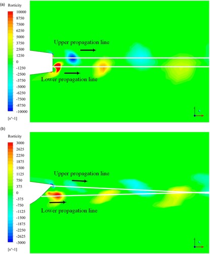
The distributions of wake vortices behind the BTE hydrofoil are shown in Figure (a), which are located on the middle section. The regions with high swirling strength are identified and visualized by rigid vorticity. The wake vortices are arranged in accordance with the classical model of Kármán vortex street, and the upper and lower vortices transport along the upper (Z≈+0.8mm) and lower (Z≈−0.8mm) propagation lines, respectively. In contrast, the distributions of wake vortices behind the DTE hydrofoil are shown in Figure (b), which are also located on the middle section. Compared with the wake vortices from the BTE, the wake vortices from the DTE transport along the asymmetric oblique lines, and the swirling strength is much lower than that of the BTE. The swirling strength of the upper vortex that is about to transport downstream is one-sixth of that of the BTE, while the swirling strength of the lower vortex that is about to transport downstream is one-tenth of that of the BTE, which shows the significant changes in local flow patterns caused by the modification of trailing edge.
Figure 4. Vortex street of the hydrofoil with different trailing edges. (a) BTE. (b) DTE.
The evolution of wake vortices marked by rigid vorticity is exactly the transport of this physical quantity. According to Equation (13), the transport of rigid vorticity is driven by different deformation terms. Taking the wake vortex of the DTE hydrofoil as a real example, the effects of these deformation terms are vividly shown in Figure . According to the real flow fields, RST (the stretching term ωR·▿V) can represent the normal strain (tension or compression) of the vortex core line. RDT (the dilatation term V▿·ωR) can represent the tangential strain (torsion or bending) of the vortex tube in the convection process. RCT (the curl term of the pseudo Lamb vector ▿×(ωR×V)) can represent the axial strain of the vortex tube and reflect the intensity change of rigid vorticity, thereby being regarded as a quasi production term in kinematics. RVT (the viscous term υeff▵ω) can represent the axial strain of the vortex tube and reflect the dissipation of rigid vorticity caused by viscous effects, especially the turbulent eddy viscosity. Moreover, for the wake flow fields of the BTE hydrofoil, the effect of each deformation term is presented in the same way. These results are consistent with the theoretical analyses in subsection 2.3.
Figure 5. A general deformation mechanism of the vortex tube. (a) RST. (b) RDT. (c) RCT. (d) RVT.
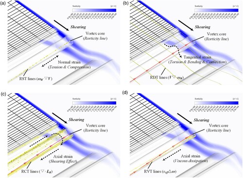
Accordingly, a general deformation process of the vortex tube is presented. This allows the deformation form of a vortex tube to be given in a way close to orthogonal decomposition, and thus the vortex spatial evolution can be described by four almost independent deformation terms. Compared with the traditional vorticity stretching term ω·▿V that integrates such deformation information as stretching, tilting, and twisting in a synthetic way (Wu et al., Citation2006), the rigid vorticity transport equation makes it easier to clearly express and understand the evolution process of turbulent vortices.
3.4 Rigid vorticity transport characteristics of the wake vortices
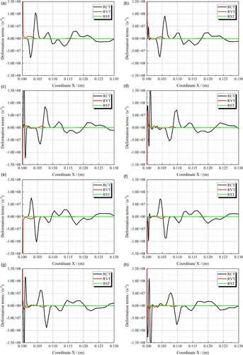
Rigid vorticity magnitude changes of a spanwise vortex tube are characterized by the stretching of the vortex line and are mainly driven by the axial strains. To further reveal the origin of the above wake vortex characteristics, the distributions of RST, RCT and RVT along the upper and lower propagation lines at four typical moments in a full period, T1∼T4, are given. As shown in Figure , for the hydrofoil with a BTE, RST has the smallest magnitude, which indicates that the normal strain of the vortex core line is very weak. In the wake vortex formation process, the magnitude of RCT is much higher than that of RVT, which implies that the production of rigid vorticity is much higher than the dissipation. This is an important reason why the wake vortices with high swirling strength can be generated from the BTE (Figure (a)), which is consistent with the experimental observations of Bourgoyne et al. (Citation2003, Citation1999). It also shows that the dissipation effect of the wake flow fields near the BTE is weak, which is not conducive to the increase in hydrodynamic damping. Moreover, with the advance of the transport process, the production effect of RCT is still dominant but constantly weakened, thereby inducing the feature of the swirling strength of the transporting wake vortex gradually decreasing.
Figure 6. Distributions of deformation terms along the propagation lines (BTE). (a) T1 (Upper). (b) T2 (Upper). (c) T3 (Upper). (d) T4 (Upper). (e) T1 (Lower). (f) T2 (Lower). (g) T3 (Lower). (h) T4 (Lower).
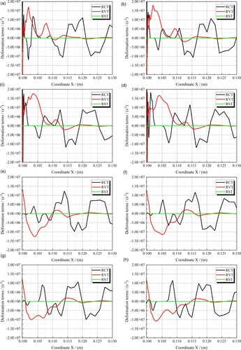
As shown in Figure , for the hydrofoil with a DTE, RST also has the smallest magnitude, which indicates that the normal strain of the vortex core line is also very weak. In the upper vortex formation process, the magnitude of RVT is close to that of RCT, which implies that the production of rigid vorticity is accompanied by high dissipation. In the lower vortex formation process, the magnitude of RVT is much higher than that of RCT, which implies that the production of rigid vorticity is much weaker. Accordingly, compared with the mature vortex from the BTE, the swirling strength of the mature vortex from the DTE is much weaker, especially the lower vortex (Figure (b)), which can be vividly described as vortex dysplasia. The dissipation effect of the wake flow fields near the DTE is strong, which is conducive to the increase in hydrodynamic damping and thus has a positive contribution to the vibration reduction of the hydrofoil. This is an intuitive explanation of the flow mechanism behind the Donaldson modification. Besides, with the advance of the transport process, the magnitude of RVT rapidly decreases, while the magnitude of RCT slightly increases, thereby inducing the feature of the swirling strength of the transporting wake vortex increasing first and then gradually decreasing.
Figure 7. Distributions of deformation terms along the propagation lines (DTE). (a) T1 (Upper). (b) T2 (Upper). (c) T3 (Upper). (d) T4 (Upper). (e) T1 (Lower). (f) T2 (Lower). (g) T3 (Lower). (h) T4 (Lower).
In summary, compared with the BTE, the dissipation of rigid vorticity exceeds the production of vortex in the wake flow fields near the DTE, which is conducive to the increase in hydrodynamic damping and directly leads to the fact that the swirling strength of the mature vortex is much weaker, and thus the unsteady vortical behavior in the wake flow fields can also be significantly weakened, which is conducive to the decrease in added mass.
4. Application case II: inverse design of a centrifugal pump impeller
4.1 Engineering background and application objective
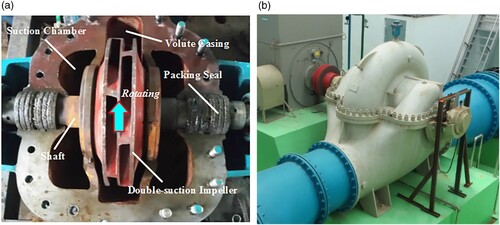
High-power centrifugal pumps are widely employed in the large-scale high-head water diversion projects and agricultural irrigation projects in China. As shown in Figure , large-scale double-suction centrifugal pumps are more prone to pressure fluctuations, which can induce severe vibration and has become a key issue in hydro-energy machinery (Yao et al., Citation2011; Zeng et al., Citation2020). According to the aforementioned studies of Das et al. (2020), low-pressure regions in the flow fields are strongly associated with rigid rotation motions (rigid vorticity ωR), while pure shearing motions (deformational vorticity ωS) are associated with nearly zero pressure fluctuations. The swirling features of vortical flows are mainly determined by rigid vorticity, and thus clarifying its transport characteristics is beneficial for controlling the pressure fluctuations, which has high engineering value. Accordingly, the second application case is discussed based on the engineering demand of guiding the inverse impeller design and improving pump stability.
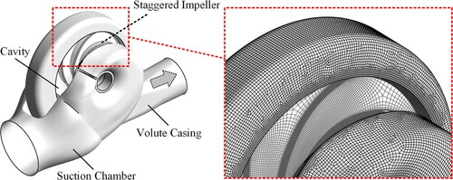
Figure 8. Geometric structures of the centrifugal pump (Wang et al., Citation2021b). (a) Double-suction impeller. (b) Double-suction pump.
4.2 V&V of numerical simulation scheme
Taking a double-suction centrifugal pump model as a typical flow case (Figure (a); He et al., Citation2015), the geometric parameters and the hydraulic parameters of this pump model are given as follows. The impeller outlet diameter and the blade number are D2=432 mm and Z=6, respectively. The rated pump head, rated pump flowrate and the rotational speed of impeller are H0=56.5m, Q0=800m3/h and n=1490rpm, respectively. The specific speed of this pump model is approximately ns = 88.
ANSYS CFX are used for numerical simulations of the flow fields, and the classical SAS-SST turbulence model is employed. As shown in Figure , the computational domain is determined according to the experiment conducted in the BIDR (He et al., Citation2015), which comprises the semi-spiral suction chamber, double-suction impeller, pump cavity, volute casing and the extension parts. The flow domains are discretized by using the high quality hexahedral grids, and the grids in the near wall region are carefully determined. Moreover, the GCI (grid convergence index) criterion recommended by ASME-FE (Celik et al., Citation2008; Oberkampf & Roy, Citation2010) is used for the convergence analyses, and the details of the URANS grids were given in the previous study of the authors (Wang et al., Citation2021a). The final meshing results are shown in Figure .
Figure 9. Computational domain of the double-suction centrifugal pump.
Transient simulations are conducted and the time step δt is 2.7778×10⁻⁴s, which is equivalent to the impeller rotating 2° in each time step. Besides, the discretization schemes of the transient term, convective term and the diffusion term are the second-order backward Euler scheme, second-order upwind scheme and the central difference scheme, respectively. The boundary conditions of the inlet, outlet and the wall surfaces are the velocity condition with a medium inlet turbulence intensity, static pressure condition and the no-slip condition, respectively. Moreover, a fully implicit coupling algorithm is employed, and the residual standard of convergence is chosen as 1.0E-5.
To guarantee the prediction accuracy of numerical computation, transient simulations corresponding to the five operating conditions, 0.8Q0∼1.2Q0, are conducted, and the surface roughness effects are taken into account by using the equivalent sand-grain roughness. The H-Q (head-flowrate) curve, the P-Q (power-flowrate) curve and the peak-to-peak values of pressure fluctuations ▵H/H0 in the volute casing can be found in the previous studies of the authors (Wang et al., Citation2021a). Under the design condition, the relative errors are less than 3%, which are kept within reasonable bounds. Accordingly, the reliability of this engineering computation scheme can be guaranteed.
4.3 Rigid vorticity transport characteristics in the original impeller
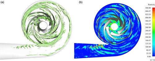
Vortical structures in the original pump are shown in Figure , which are identified and visualized by rigid vorticity. In the impeller passages, vortical structures exist near the blade suction surfaces. In the vaneless region near the impeller outlet, a large number of wake vortex tubes with high swirling strength are clearly presented, which are the important sources inducing pressure fluctuations in the volute casing.
Figure 10. Vortical structures in the original centrifugal pump (1.0Q0). (a) Rigid vorticity isosurfaces (||ωR||2=300s−1). (b) Rigid vorticity contours.
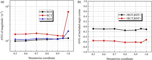
To understand the vortex transport characteristics in the original impeller domain, the distributions of rigid vorticity deformation terms along the streamwise direction are shown in Figure , which are corresponding to the radial coordinates 2r/D2=0.5∼1.0. On the different streamwise cross sections, RST has the smallest magnitude, which indicates that the normal strain of the vortex core line is very weak. The magnitude of RVT is very high in the near wall region, but it is very low in the main flow region (Re≫1). Accordingly, for the far fields outside the boundary layers where the turbulent flows are at the inviscid level but not the irrotational level, rigid vorticity transport is mainly driven by RDT, RCT and ROT, and the high magnitudes of these terms exist near the blade suction surfaces, which reflects the non-uniformity in space. Moreover, the changes in the three deformation terms along the streamwise direction are shown in Figure . For the average values on the streamwise cross sections (Figure (a)), the effect of each term is relatively steady in the range of 0.5 ≤ 2r/D2≤0.95, but RCT increases sharply near the impeller outlet (0.95 ≤ 2r/D2≤1.0), reflecting the rapid production of rigid vorticity in this region. The values of the included angle (or the vector angle) between RDT and another two terms are shown in Figure (b), representing the action mode along the streamwise direction (the vector direction of RDT is parallel to the local velocity vector). The value of < ROT,RDT > is approximately −0.1 (95.7°), which indicates that ROT is almost orthogonal to RDT. The value of < RCT,RDT > is approximately −0.6 (126.9°), which indicates that a large part of RCT is in balance with RDT. Accordingly, RCT (production effect) and ROT (Coriolis effect) play a continuous and stable role in the transport process of rigid vorticity in the centrifugal pump impeller domain.
Figure 11. Distributions of the deformation terms in the original impeller domain. (a) RST. (b) RDT. (c) RCT. (d) RVT. (e) ROT.
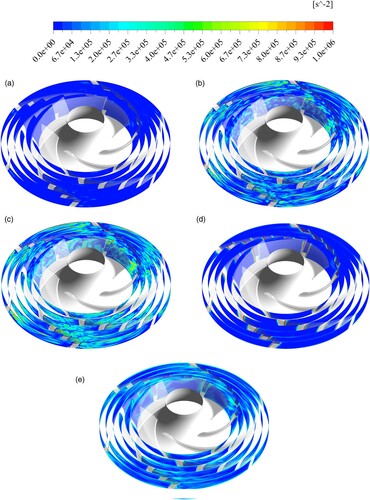
Figure 12. Changes of deformation terms along the streamwise direction. (a) Magnitudes. (b) Included angle cosine.
4.4 Impeller improvement based on rigid vorticity transport characteristics
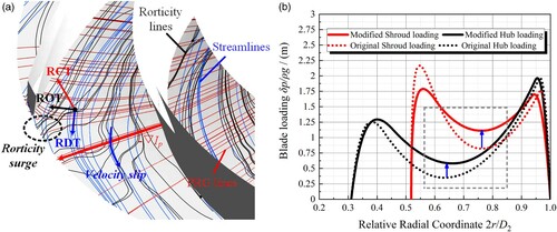
Rigid vorticity surge near the blade suction surface at the impeller outlet (Figure (b)) can increase the non-uniformity of exit vortical flows, which is harmful to the control of pressure fluctuations. As shown in Figure (a), on the S1 streamsurface near the hub, the synthetveric effects of RCT, RDT and ROT are exactly to transport the rigid vorticity to the blade suction surface. Near the impeller outlet, the velocity slip can strengthen the production effect of RCT (Figure (a)), which is the direct cause of rigid vorticity surge and severe jet-wake structure. The intuitive mechanism of it is as follows. According to the previous studies of the authors (Wang et al., Citation2021a), the incompressible momentum equation of relative motions in a centrifugal pump impeller can be given by
(14)
(14) where Ip is the potential rothalpy proposed by Wu (Citation1952). It has been demonstrated that the gradient of Ip (referred to as PRG) actively induces the vortical flows in impeller passages and can be regarded as the most significant dynamic source. At the impeller outlet, the effect of PRG rapidly weakens as the difference of Ip decreases, and thus the Coriolis effect is gradually dominant, which induces the velocity slip and cannot be completely eliminated. According to the Biot-Savart law, if the maximum PRG is too close to the impeller outlet, a larger velocity slip gradient can further promote the production effect of RCT on rigid vorticity surge, easily leading to more pressure fluctuations. This is an important relationship between the transport characteristics of rigid vorticity and the work mode of impeller, and it can be used to guide the improvement of blade loading and the control of vortical flows. The theoretical distributions of the blade loading δp of the original impeller, which is defined as the difference in static pressure p between the blade pressure surface and the blade suction surface, are adjusted according to this guiding principle. As shown in Figure (b), the values of δp in the middle part of the S2 streamsurface are appropriately improved to make the maximum PRG move backwards. More details of the modified impeller can be found in the previous study of the authors (Wang et al., Citation2021a).
Figure 13. Improvement scheme of the original pump impeller. (a) Rigid vorticity surge. (b) Theoretical blade loading.
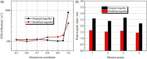
A performance comparison between the original and the modified schemes is shown in Figure . Under the design condition, the standard deviation distributions of rigid vorticity ||ωR||2 along the streamwise direction are shown in Figure (a). The results show that the standard deviation of rigid vorticity at the modified impeller outlet is reduced by 55.13%, and thus the exit uniformity of rigid vorticity is significantly improved. Peak-to-peak values of pressure fluctuations ▵H are shown in Figure (b). It is found that the peak-to-peak values of pressure fluctuations are suppressed by up to 39.90%, and this improvement in pump stability was also demonstrated by a proof experiment conducted in BIDR (He et al., Citation2015; Wang et al., Citation2021a). In summary, the guiding significance and engineering value of the rigid vorticity transport equation for vortical flow analysis and control are preliminarily presented.
Figure 14. Performance comparison between the original and the modified schemes (1.0Q0). (a) Standard deviation of rigid vorticity. (b) Pressure fluctuations in volute casing.
5. Summary and conclusions
In this study, the vorticity decomposition scheme is introduced, and the rigid vorticity transport equation is proposed for the analysis and control of vortical flows in hydro-energy machinery. The main conclusions are drawn as follows.
The idea of vorticity binary decomposition indicates that total vorticity ω can be further decomposed into the rigid vorticity ωR and the deformational vorticity ωS. The rigid vorticity can be used to identify the vortex region that is characterized by rigid rotation motions. On the basis of this idea, the effects of deformational vorticity on rigid vorticity are further discussed, and then the rigid vorticity transport equation is proposed.
In the rigid vorticity transport equation, vortex spatial evolution in the main flow region is described by the stretching term RST, the dilatation term RDT, the Lamb term RCT and the viscous term RVT. ROT appears as a natural term in the impeller domains. The shape change of a vortex tube is mainly affected by RST and RDT, and the vortex production and dissipation are mainly reflected by RCT and RVT.
For the first application case, the results show that vorticity dissipation RVT is much higher than vortex production RCT in the wake flow fields near the DTE, while the BTE hydrofoil is the opposite. This reveals the direct reason for greater hydrodynamic damping of the Donaldson hydrofoil.
For the second application case, the results show that the induction effect of RCT on vortex surge can be promoted by unreasonable blade loading near the pump impeller outlet. According to this guiding principle, the original scheme is improved. The standard deviation of rigid vorticity at the modified impeller outlet is reduced by 55.13%, and the peak-to-peak values of pressure fluctuations in the volute casing are reduced by 39.90%. This improvement in pump stability is also demonstrated by a proof experiment.
Overall, the engineering value of the rigid vorticity transport equation has been preliminarily presented, and it can provide a practical method for the vortical structure evolution analysis in hydro-energy machinery. In the future, more engineering cases should be studied by using more advanced computation methods. On the one hand, the advantages of this theoretical tool in turbulent flow analysis can be further explored. On the other hand, this tool can be further developed to guide the control of vortical flows in hydraulic engineering.
Disclosure statement
No potential conflict of interest was reported by the author(s).
Additional information
Funding
References
- Astarita, G. (1979). Objective and generally applicable criteria for flow classification. Journal of Non-Newtonian Fluid Mechanics, 6(1), 69–76. https://doi.org/https://doi.org/10.1016/0377-0257(79)87004-4
- Ausoni, P. (2009). Turbulent vortex shedding from a blunt trailing edge hydrofoil. Swiss Federal Institute of Technology Lausanne: Ph.D. dissertation.
- Bourgoyne, D. A., Ceccio, S. L., & Dowling, D. R. (1999). Vortex shedding from a hydrofoil at high Reynolds number. Journal of Fluid Mechanics, 531, 293–324. https://doi.org/https://doi.org/10.1017/S0022112005004076
- Bourgoyne, D. A., Hamel, J. M., Ceccio, S. L., & Dowling, D. R. (2003). Time-average flow over a hydrofoil at high Reynolds number. Journal of Fluid Mechanics, 496, 365–404. https://doi.org/https://doi.org/10.1017/S0022112003006190
- Celik, I. B., Ghia, U., Roache, P. J., Freitas, C. J., Coleman, H., & Raad P, E. (2008). Procedure for estimation and reporting of uncertainty due to discretization in CFD applications. Journal of Fluids Engineering, 130(7), 078001. https://doi.org/https://doi.org/10.1115/1.2960953
- Chong, M. S., Perry, A. E., & Cantwell, B. T. (1990). A general classification of three-dimensional flow fields. Physics of Fluids A: Fluid Dynamics, 2(5), 765–777. https://doi.org/https://doi.org/10.1063/1.857730
- Cuissa, J. R. C., & Steiner, O. (2020). Vortices evolution in the solar atmosphere: A dynamical equation for the swirling strength. Astronomy & Astrophysics, 639, A118. https://doi.org/https://doi.org/10.1051/0004-6361/202038060
- Das, R., & Girimaji, S. S. (2020a). Characterization of velocity-gradient dynamics in incompressible turbulence using local streamline geometry. Journal of Fluid Mechanics, 895, A5. https://doi.org/https://doi.org/10.1017/jfm.2020.286
- Das, R., & Girimaji, S. S. (2020b). Revisiting turbulence small-scale behavior using velocity gradient triple decomposition. New Journal of Physics, 22(6), 063015. https://doi.org/https://doi.org/10.1088/1367-2630/ab8ab2
- Donaldson, R. M. (1956). Hydraulic turbine runner vibration. Journal of Engineering for Power, 78, 1141–1147.
- Dörfler, P., Sick, M., & Coutu, A. (2013). Flow-induced pulsation and vibration in hydroelectric machinery. Springer-Verlag.
- Dreyer, M., Decaix, J., Münch-Alligné, C., & Farhat, M. (2014). Mind the gap: A new insight into the tip leakage vortex using stereo-PIV. Experiments in Fluids, 55(11), 1849. https://doi.org/https://doi.org/10.1007/s00348-014-1849-7
- Gao, Y. S., & Liu, C. Q. (2019). Rortex based velocity gradient tensor decomposition. Physics of Fluids, 31(1), 011704. https://doi.org/https://doi.org/10.1063/1.5084739
- Ghalandari, M., Shamshirband, S., Mosavi, A., & Chau, K. W. (2019). Flutter speed estimation using presented differential quadrature method formulation. Engineering Applications of Computational Fluid Mechanics, 13(1), 804–810. https://doi.org/https://doi.org/10.1080/19942060.2019.1627676
- He, C. L., Jiang, Y. H., Zhang, Z. B., Zhang, Y. Y., & Yan, Y. (2015). Double-suction centrifugal pump model test report for China Agricultural University. China Water Beifang Investigation, Design and Research Co. Ltd.
- Hu, J., Wang, Z. B., Chen, C. G., & Guo, C. Y. (2020). Vortex shedding simulation of hydrofoils with trailing-edge truncation. Ocean Engineering, 214, 107529. https://doi.org/https://doi.org/10.1016/j.oceaneng.2020.107529
- Jeong, J., & Hussain, F. (1995). On the identification of a vortex. Journal of Fluid Mechanics, 285(-1), 69–94. https://doi.org/https://doi.org/10.1017/S0022112095000462
- Jiang, D. Z. (1999). Vorticity decomposition and its application to sectional flow characterization. Tectonophysics, 301(3-4), 243–259. https://doi.org/https://doi.org/10.1016/S0040-1951(98)00246-7
- Kolář, V., & Šístek, J. (2020). Consequences of the close relation between Rortex and swirling strength. Physics of Fluids, 32(9), 091702. https://doi.org/https://doi.org/10.1063/5.0023732
- Kolář, V. (2007). Vortex identification: New requirements and limitations. International Journal of Heat and Fluid Flow, 28(4), 638–652. https://doi.org/https://doi.org/10.1016/j.ijheatfluidflow.2007.03.004
- Lindgren, E. R. (1980). Vorticity and rotation. American Journal of Physics, 48(6), 465–467. https://doi.org/https://doi.org/10.1119/1.12083
- Liu, C. Q., Gao, Y. S., Dong, X. R., Wang, Y. Q., Liu, J. M., Zhang, Y. N., Cai, X. S., & Gui, N. (2019). Third generation of vortex identification methods: Omega and Liutex/Rortex based systems. Journal of Hydrodynamics, 31(2), 205–223. https://doi.org/https://doi.org/10.1007/s42241-019-0022-4
- Liu, C. Q., Gao, Y. S., Tian, S. L., & Dong, X. R. (2018). Rortex-A new vortex vector definition and vorticity tensor and vector decompositions. Physics of Fluids, 30(3), 034103. https://doi.org/https://doi.org/10.1063/1.5018844
- Nennemann, B., & Monette, C. (2018). Prediction of vibration amplitudes on hydraulic profiles under von Karman vortex excitation. 29th IAHR Symposium on Hydraulic Machinery and Systems.
- Oberkampf, W. L., & Roy, C. J. (2010). Verification and validation in scientific computing. Cambridge University Press.
- Pasche, S., Avellan, F., & Gallaire, F. (2017). Part load vortex rope as a global unstable mode. Journal of Fluids Engineering, 139(5), 051102. https://doi.org/https://doi.org/10.1115/1.4035640
- Robinson, S. K., Kline, S. J., & Spalart, P. R. (1989). A review of quasi-coherent structures in a numerically simulated turbulent boundary layer. NASA Technical Reports Server: NASA-TM-102191.
- Salih, S. Q., Aldlemy, M. S., Rasani, M. R., Ariffin, A. K., Ya, T. M. Y. S. T., Al-Ansari, N., Yaseen, A. M., & Chau, K. W. (2019). Thin and sharp edges bodies-fluid interaction simulation using cut-cell immersed boundary method. Engineering Applications of Computational Fluid Mechanics, 13(1), 860–877. https://doi.org/https://doi.org/10.1080/19942060.2019.1652209
- Sun, B. H. (2019). A new additive decomposition of velocity gradient. Physics of Fluids, 31(6), 061702. https://doi.org/https://doi.org/10.1063/1.5100872
- Tian, S. L., Gao, Y. S., Dong, X. R., & Liu, C. Q. (2018). Definitions of vortex vector and vortex. Journal of Fluid Mechanics, 849, 312–339. https://doi.org/https://doi.org/10.1017/jfm.2018.406
- Trivedi, C. (2017). A review on fluid structure interaction in hydraulic turbines: A focus on hydrodynamic damping. Engineering Failure Analysis, 77, 1–22. https://doi.org/https://doi.org/10.1016/j.engfailanal.2017.02.021
- Truesdell, C. (1954). The kinematics of vorticity. Indiana University Press.
- Wang, C. Y., Wang, F. J., An, D. S., Yao, Z. F., Xiao, R. F., Lu, L., He, C. L., & Zou, Z. C. (2021a). A general alternate loading technique and its applications in the inverse designs of centrifugal and mixed-flow pump impellers. Science China-Technological Sciences, 64(4), 898–918. https://doi.org/https://doi.org/10.1007/s11431-020-1687-4
- Wang, C. Y., Wang, F. J., Tang, Y., Wang, B. H., Yao, Z. F., & Xiao, R. F. (2020). Investigation on the horn-like vortices in stator corner separation flow in an axial flow pump. Journal of Fluids Engineering, 142(7), 071208. https://doi.org/https://doi.org/10.1115/1.4046376
- Wang, C. Y., Wang, F. J., Xie, L. H., Wang, B. H., Yao, Z. F., & Xiao, R. F. (2021b). On the vortical characteristics of horn-like vortices in stator corner separation flow in an axial flow pump. Journal of Fluids Engineering, 143(6), 061201. https://doi.org/https://doi.org/10.1115/1.4049687
- Wang, Y. Q., Gao, Y. S., Liu, J. M., & Liu, C. Q. (2019). Explicit formula for the Liutex vector and physical meaning of vorticity based on the Liutex-Shear decomposition. Journal of Hydrodynamics, 31(3), 464–474. https://doi.org/https://doi.org/10.1007/s42241-019-0032-2
- Wang, Z. Y., Huang, B., Zhang, M. D., Wang, G. Y., & Zhao, X. A. (2018). Experimental and numerical investigation of ventilated cavitating flow structures with special emphasis on vortex shedding dynamics. International Journal of Multiphase Flow, 98, 79–95. https://doi.org/https://doi.org/10.1016/j.ijmultiphaseflow.2017.08.014
- Wedgewood, L. E. (1999). An objective rotation tensor applied to non-Newtonian fluid mechanics. Rheologica Acta, 38(2), 91–99. https://doi.org/https://doi.org/10.1007/s003970050159
- Wu, C. H. (1952). A general theory of three-dimensional flow in subsonic and supersonic turbomachines of axial-, radial-, and mixed-flow types. NASA Technical Reports Server: NACA-TN-2604.
- Wu, J. Z., Ma, H. Y., & Zhou, M. D. (2006). Vorticity and vortex dynamics. Springer-Verlag.
- Yamamoto, K., Müller, A., Favrel, A., & Avellan, F. (2017). Experimental evidence of inter-blade cavitation vortex development in francis turbines at deep part load condition. Experiments in Fluids, 58(10), 142. https://doi.org/https://doi.org/10.1007/s00348-017-2421-z
- Yao, Z. F., Wang, F. J., Dreyer, M., & Farhat, M. (2014). Effect of trailing edge shape on hydrodynamic damping for a hydrofoil. Journal of Fluids and Structures, 51, 189–198. https://doi.org/https://doi.org/10.1016/j.jfluidstructs.2014.09.003
- Yao, Z. F., Wang, F. J., Qu, L. X., Xiao, R. F., He, C. L., & Wang, M. (2011). Experimental investigation of time-frequency characteristics of pressure fluctuations in a double-suction centrifugal pump. Journal of Fluids Engineering, 133(10), 1076–1081. https://doi.org/https://doi.org/10.1115/1.4004959
- Ye, C. L., Wang, F. J., Wang, C. Y., & Bart, P. M. E. (2020). Assessment of turbulence models for the boundary layer transition flow simulation around a hydrofoil. Ocean Engineering, 217, 108124. https://doi.org/https://doi.org/10.1016/j.oceaneng.2020.108124
- Zeng, Y. S. (2018). Numerical simulation of the effect of tailing edge shape on hydrodynamic damping characteristics for a hydrofoil. China Agricultural University: Master dissertation.
- Zeng, Y. S., Yao, Z. F., Wang, F. J., Xiao, R. F., & He, C. L. (2020). Experimental investigation on pressure fluctuation reduction in a double suction centrifugal pump: Influence of impeller stagger and blade geometry. Journal of Fluids Engineering, 142(4), 041202. https://doi.org/https://doi.org/10.1115/1.4045208
- Zeng, Y. S., Yao, Z. F., Zhou, P. J., Wang, F. J., & Hong, Y. P. (2019). Numerical investigation into the effect of the trailing edge shape on added mass and hydrodynamic damping for a hydrofoil. Journal of Fluids and Structures, 88, 167–184. https://doi.org/https://doi.org/10.1016/j.jfluidstructs.2019.05.006
- Zhan, J. M., Chen, Z. Y., Li, C. W., Hu, W. Q., & Li, Y. T. (2020). Vortex identification and evolution of a jet in cross flow based on Rortex. Engineering Applications of Computational Fluid Mechanics, 14(1), 1237–1250. https://doi.org/https://doi.org/10.1080/19942060.2020.1816496
- Zhan, J. M., Li, Y. T., Wai, W. H. O., & Hu, W. Q. (2019). Comparison between the Q criterion and Rortex in the application of an in-stream structure. Physics of Fluids, 31(12), 121701. https://doi.org/https://doi.org/10.1063/1.5124245
- Zhang, Y. N., Zhang, Y. N., & Wu, Y. L. (2017). A review of rotating stall in reversible pump turbine. Proceedings of the Institution of Mechanical Engineers, Part C: Journal of Mechanical Engineering Science, 231(7): 1181–1204. https://doi.org/https://doi.org/10.1177/0954406216640579
- Zhao, X. R., Xiao, Y. X., Wang, Z. W., Luo, H. Y., Ahn, S. H., Yao, Y. Y., & Fan, H. G. (2017). Numerical analysis of non-axisymmetric flow characteristic for a pump-turbine impeller at pump off-design condition. Renewable Energy, 115, 1075–1085. https://doi.org/https://doi.org/10.1016/j.renene.2017.06.088
- Zhou, J., Adrian, R. T., Balachandar, S., & Kendall, T. M. (1999). Mechanisms for generating coherent packets of hairpin vortices in channel flow. Journal of Fluid Mechanics, 387, 353–396. https://doi.org/https://doi.org/10.1017/S002211209900467X
- Zobeiri, A. (2012). Effect of hydrofoil trailing edge geometry on the wake dynamics. Swiss Federal Institute of Technology Lausanne: Ph.D. dissertation.
- Zobeiri, A., Ausoni, P., Avellan, F., & Farhat, M. (2012). How oblique trailing edge of a hydrofoil reduces the vortex-induced vibration. Journal of Fluids and Structures, 32, 78–89. https://doi.org/https://doi.org/10.1016/j.jfluidstructs.2011.12.003
Appendix
In subsection 2.2, to give a general expression between e[Ω] and e[R] (two SO(3) orthogonal rotation tensors), we need to clarify the motion trend of a fluid element.
Firstly, yawing (the basic definition of this Euler attitude is that the rotational or oscillatory movement of an aircraft or similar body about its vertical axis.) and pitching (the basic definition of this Euler attitude is that the rotational or oscillatory movement of an aircraft or similar body about its lateral axis.) caused by the normal shearing effects (ω1 and ω2) can cause the QZ-axis and Z-axis (rigid rotation axis) to be misaligned. Thus, the first Euler transformation matrix C can be adopted to transform the original [Q] system into a new [Q1] system, in which the Q1Z-axis is aligned with the Z-axis of the BRF. According to the theory of rigid body dynamics (Tian et al., Citation2018), the rotation matrix C and the new tensor [Q1] are expressed as
(A1)
(A1)
where Q31, Q32 and Q33 are the elements of the third column vector of [Q] (the components of the QZ vector), and the elements M1 and M2 of [Q1] are given by
(A2)
(A2)
which implies that residual effects of normal shearing (ω1 and ω2) still exist.
Secondly, another Euler transformation matrix B is required to transform the [Q1] system into a new [Q2] system, in which the rolling trend (the basic definition of this Euler attitude is that the rotational or oscillatory movement of an aircraft or similar body about its longitudinal axis.) of a fluid element can only result from the effects of rigid rotation and tangential shearing (ω3). This change process is expressed as
(A3)
(A3)
where the elements M3 and M4 of the rotation matrix B are given by
(A4)
(A4)
Thirdly, another Euler transformation matrix A can be employed to transform the [Q2] system into a new [Q3] system, in which the rolling trend around the Z-axis is only caused by the rigid rotation effect (rigid vorticity). This change process is expressed as
(A5)
(A5)
For a fluid element, a general mathematical relationship between the e[Ω] (vorticity) and the e[R] (rigid vorticity) can be expressed as ABC[Q] = e[R], which directly reveals the motion trend under the actions of rigid rotation (φ) and pure shearing (s, ξ, and η). Actually, it also shows the effects of pure shearing motions on rigid rotation motions of local fluids.
Nomenclature
| ω (▿×V) | = | Vorticity (Velocity curl) |
| ωR | = | Rigid vorticity (Rorticity) |
| ωS | = | Deformational vorticity |
| ▿V | = | Velocity gradient tensor |
| r | = | Direction vector of the rigid rotation axis |
| XYZ | = | Basic reference frame (BRF) |
| λcr, λr | = | Normal strain |
| s, ξ, η | = | Pure shearing |
| φ | = | Angular velocity of rigid rotation |
| [R] | = | Rigid rotation rate tensor |
| [ε] | = | Levi-Civita permutation tensor |
| λci | = | Swirling strength |
| SO(3) | = | Three dimensional rotation group |
| [Ω] | = | Rotation rate tensor |
| [Q] | = | Natural exponential function of [Ω] |
| δij | = | Kronecker delta |
| εijk | = | Levi-Civita symbol |
| υ | = | Kinematic viscosity |
| f | = | Body force |
| ρ | = | Density |
| p | = | Static pressure |
| LR | = | Pseudo Lamb vector |
| RST | = | Rigid vorticity stretching term |
| RDT | = | Rigid vorticity dilatation term |
| RCT | = | Curl term of LR |
| RVT | = | Viscous term |
| ROT | = | Coriolis term |
| Re | = | Reynolds number |
| BTE | = | Blunt trailing edge |
| DTE | = | Donaldson trailing edge |
| D2 | = | Impeller outlet diameter |
| H0 | = | Rated pump head |
| Q0 | = | Rated pump flowrate |
| n | = | Rotational speed of impeller |
| ns (3.65nQ | = | Specific speed (Chinese Standard) |
| = | ||
| Vr | = | Relative velocity |
| Ip | = | Potential rothalpy |
| PRG | = | Potential rothalpy gradient |
| ωi | = | Angular velocity of impeller |
| δp | = | Blade loading |