Seismic performance analysis of a wind turbine with a monopile foundation affected by sea ice based on a simple numerical method

Abstract

To investigate the seismic performance of a wind turbine that is influenced by both the ice load and the seismic load, the research proposes a numerical approach for simulating the seismic behavior of a wind turbine on a monopile foundation. First, the fluid–solid coupled equation for the water–ice–wind turbine is simplified by assigning reasonable boundary conditions and solving the motion equation, and the seismic motion equation of the wind turbine is developed. Then, on this basis, we propose a simplified 3D numerical model that can simulate the interactions among the wind turbine, water and sea ice. By conducting shaking table tests, the results demonstrate that the established numerical model is effective. Finally, we investigate the effect of the boundary range and ice thickness on the seismic performance of a turbine under near-field and far-field seismic actions. Research results illustrate that ice changes the distribution form of the hydrodynamic pressure. Moreover, the thickness of the ice greatly influences the seismic behavior, while the influence of the ice boundary range is only within a certain range. Additionally, the ice load decreases the energy-dissipating capacity of the wind turbine, so the earthquake resilience of the wind turbine is significantly decreased.

KEYWORDS:

• Sea ice
• wind turbine
• 3D numerical model
• seismic performance
• shaking table test

1. Introduction

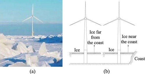
Most offshore structures in global cold regions are basically covered by ice that can be as thick as several meters (Hacıefendioğlu et al., 2009). The coastal areas of China lie in the circum-Pacific earthquake zone, and offshore structures built in these areas are influenced by both a seismic load and an ice load. Sea ice of different sizes and thicknesses driven by an earthquake can cause lateral vibration of the structure and can trigger serious structural hazards, economic losses and fatalities. For example, numerous coastal bridge piers were damaged in the 1964 Alaska earthquake (M9.1) due to the combined effects of ice and the earthquake (Qi & Song, 2013). In recent years, due to serious environmental problems and the demand for clean energy, many offshore wind turbines have been built in China. The service environment of the wind turbines is complex, and it is affected by many factors (Chen & Lian, 2015; Meana-Fernández et al., 2019; Quezada et al., 2018). When considering external loads in wind turbine design, the ice load is one of the important factors affecting the wind turbine’s safety (Figure 1(a)) (Shamaei et al., 2020). There are two forms of ice in the sea, i.e. that near the coast and that far from the coast; and sea ice far from the coast imposes a greater effect on the structure (Figure 1(b)). Consequently, determining the seismic performance of a wind turbine structure affected by sea ice is quite important for ensuring the safety of the wind turbine and its future service (Withalm & Hoffmann, 2010).

Figure 1. Wind turbine in water containing sea ice: (a) wind turbine surrounded by ice; (b) two forms of ice.

The threat of ice to ocean structures has been of widespread concern owing to its evident dynamic effects. Using three methods, i.e. integrated, weakly coupled and fully coupled approaches, Yu et al. (2021) investigated ice–structure interactions. Nevertheless, the coupling of water and ice and the seismic load are not considered jointly in these approaches. Zhu et al. (2021) developed a simulation program to investigate ice–structure interactions based on Määttänen–Blenkarn’s model. However, one major outstanding issue exists in this simulation program; that is, the ice force is considered as an independent dynamic system, and the ice–structure interactions are only explained by the frequency-locking phenomenon. Therefore, this simulation program cannot be used for the dynamic nonlinear analysis of structures under seismic action. Heinonen and Rissanen (2017) studied the effect of ice–structure interactions upon a wind turbine in terms of its structural performance using simulation software and demonstrated that coupling simulation of the ice and structure is a necessary step to reducing the construction costs of a structure. Under earthquake activity, the sea ice around the structure vibrates with this structure, and the structure’s seismic behavior is affected. As a random vibration load, earthquakes further complicate the ice–structure interaction. Jia (2010) and Qi and Song (2013) considered the combined action of seismic and ice loads and investigated the dynamic response of the piers and bridge. Their research results revealed that the combined action of the seismic load and the ice load obviously affects the displacement and internal force of the pier. In addition, the hydrodynamic pressure induced by the earthquake was also considered in these studies. Consequently, the combined action of the seismic load and the ice load and the earthquake-induced hydrodynamic pressure all have effects on the structure that should not be ignored. Unfortunately, in the existing approaches, the hydrodynamic pressure is usually calculated using Morison’s equation, and the structure and ice are often simplified to lumped masses, and the interactions between them are simulated using springs and damping (Huang et al., 2021). It should be noted that the effects of size and thickness of the ice on the structure cannot be taken into consideration using these simplified methods.

Although remarkable progress toward understanding ice–structure and ice–water interactions has been made in previous studies, few studies have taken seismic loads into account, which is a potential threat to wind turbines in earthquake-prone areas. Earthquake-induced hydrodynamic pressure is also an important factor in structural design. Jia and Han (2011) concluded that the presence of ice exerts certain influences upon hydrodynamic pressure. Kobayashi (2002) also put forward the idea that the influence from sea ice amplifies the hydrodynamic pressure, and the ice–water interplay effect cannot be ignored. Therefore, the water–ice–structure interactions should also be considered in seismic performance analysis. Ramezanizadeh et al. (2019) pointed out that the ice–water–structure interactions are a fluid–solid coupling problem; however, it is difficult to obtain a coupled fluid–solid analytical solution due to the complexity of the coupling. Consequently, although simplified approaches for calculating hydrodynamic pressure and ice loads are available in design standards (ISO-19906, 2010; Risk & Bridges, 2019), earthquake activity creates a challenge in the use of these methods (Hendrikse & Nord, 2019) because the effect of the ice load is replaced by the maximum static ice force in these methods. As a result, these methods are not applicable to the analysis of the dynamic characteristics of structures subjected to earthquake activity. Many scholars have attempted to establish an ice force model to simulate the mechanical behavior of ice. At present, widely-used ice force models mainly include the Matlock model (Withalm & Hoffmann, 2010), the Karna model (Karna & Turnunen, 1990) and the Croteau model (1983). Some scholars have continued to improve these ice force models. Shi et al. (2001), Yue et al. (2003) and Wang (2014) improved the governing ice force function and the parameters of the ice force model, but they did not consider the physical and mechanical properties of ice when determining the ice crushing length. Xiangjun et al. (2006), Brown and Morsy (1995) and Bouaanani et al. (2004) improved the substructure model based on different crushing models and sea-ice criteria; however, there is no uniform formula for calculating the ice force in these models. In fact, the dynamic ice force models mentioned above are relatively simple and are a feasible method of simulating the mechanical behavior of ice, but they cannot be used to simulate the influences of the three-dimensional geometric characteristics (ice boundary range and thickness) on the wind turbine under earthquake activity. Therefore, an approach to analysing water–ice–wind turbine interaction should be established first when we investigate the seismic performance of wind turbines that are simultaneously affected by a seismic load and an ice load.

The remainder of the research is organized in the following manner: Section 2 simplifies the fluid–solid coupling equation for the water–ice–structure interactions, derives the seismic motion equation and presents a simplified numerical method for establishing a numerical model of water–ice–wind turbine interactions. In Section 3, our proposed simplified numerical method for water–ice–wind turbine interactions is validated. In Section 4, the effects of the boundary range and thickness of the ice upon the seismic responses of the structure to far-field and near-field seismic activity are investigated. In Section 5, the major conclusions of this study are presented. The results of this study provide a method for establishing a numerical model of water–ice–structure interactions and for the clarifying seismic performance of a wind turbine on the basis of the fluid–solid coupling method.

2. Numerical model for the water–ice–wind turbine interaction

2.1. Proposed simplified numerical method

At present, obtaining an analytical solution to fluid–solid coupling is still challenging when considering the interactions of wind turbines, sea ice and water. Therefore, it is necessary to simplify the coupling equation in a reasonable fashion. In order to couple the fluid (water) and the solids (ice and wind turbine), the governing equations of the fluid, solids and their interfaces are established first. For the dynamically coupled water–ice–structure system, the water needs to satisfy the equation of motion and the boundary conditions. In addition, the water is assumed to experience no heat transfer, be compressed, and induce a small disturbance; and the free surface of the fluid fluctuates marginally. Moreover, the sea ice is assumed to be a linear elastic medium (Dong et al., 2010).

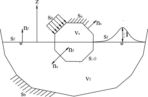
In Figure 2, $v_s$ and $v_f$ are the solid (wind turbine and ice) and the fluid domains, respectively; $s_0$ is the fluid–solid interface; and $s_b$ is the fluid rigid fixed surface boundary. $s_f$, $\xi$, $s_{\sigma }$, $n_f$ and $n_s$ are the free surface boundary of the fluids, the wave height on the fluid free surfaces, the displacement boundary of the solid, the unit normal vector of the fluid boundaries, and the unit outer normal vector of the solid, respectively. At any point on the coupled surface of the fluid and solid, $n_f$ and $n_s$ are always in opposite directions.

Figure 2. Sketch of the coupled fluid–solid system.

In the fluid and solid domains, the flow field pressure $p$ and the displacement $u$ are used as basic unknown quantities. The fluid should satisfy Equation (1) (1) $\begin{array}{r}{p}_{,\ddot{u}}-\frac{1}{c_0^2}\ddot{p}=0\end{array}$(1) where $c_0$ is the transmission velocity of sound in a fluid. The boundary conditions of the fluid satisfy Equations (2) and (3).

Free surface $\left(s_f\right)$: (2) $\begin{array}{r}\frac{\mathrm{\partial }p}{\mathrm{\partial }z}+\frac{1}{g}\ddot{p}=0\end{array}$(2) Fixed interface $\left(s_b\right)$: (3) $\begin{array}{r}\frac{\mathrm{\partial }p}{\mathrm{\partial }{n}_f}=0\end{array}$(3) From the above equations, we can see that there is only a single variable (the pressure $p$) at each node in the model, and thus the computational efficiency can be improved. For the solid domain, Equation (4) should be satisfied: (4) $\begin{array}{r}{\sigma }_{ij,j}+f_i={\rho }_s{\ddot{u}}_i\end{array}$(4) where ${\sigma }_{ij,j}$, $u_i$ and $f_i$ are the components of the solid stress, solid displacement and solid volume force, respectively; ${\rho }_s$ denotes the mass density of the solid. The boundary conditions of the solid domain satisfy Equations (5) and (6).

Force boundary condition $\left(s_{\sigma }\right)$: (5) $\begin{array}{r}{\sigma }_{ij}{n}_{sj}={\overline{T}}_i.\end{array}$(5) Displacement boundary condition $\left(s_u\right)$: (6) $\begin{array}{r}{u}_n=u_i{n}_i\end{array}$(6) where ${\overline{T}}_i$ is the surface force component and $u_i$ is the displacement component in the solid domain, which are known quantities.

The kinematic and continuous boundary conditions at the coupled surface of the fluid and solid should be satisfied. The kinematic boundary condition is that the normal velocity on the coupled surface of the fluid and solid $\left(s_0\right)$ should remain continuous (Equation 7). The force continuous boundary condition is that, on the fluid–solid interface, the normal force should be continuous (Equation 8): (7) $\begin{array}{rl}{v}_{fn}& =v_f{n}_f=-v_s{n}_s=v_{sn}\end{array}$(7) (8) $\begin{array}{rl}{\sigma }_{ij}{n}_{sj}& ={\tau }_{ij}{n}_{ij}=-{\tau }_{ij}{n}_{sj}\end{array}$(8) where ${\tau }_{ij}$ is a component of the solid shear stress. The pressure distribution in the fluid element can be calculated using Equation (9): (9) $\begin{array}{r}{p}_f(x,y,z,t)=\sum _{i=1}^{m_f}{N}_i(x,y,z){p^e}_i\left(t\right)=N{p}^e\end{array}$(9) where $m_f$, $p^e$, $N_i$ and $N$ are the node number of the fluid element, the nodal pressure on each element, the difference function corresponding to node i and the shape function of the pressure element, respectively.

The displacement distribution in the solid element can be calculated using Equation (10): (10) $\begin{array}{rl}u(x,y,z,t)& =\left[\begin{array}{c}u\\ v\\ w\end{array}\right]\approx \sum _{i=1}^{m_s}{N}_i(x,y,z)\left[\begin{array}{c}{u}_i\\ v_i\\ w_i\end{array}\right]\\ & =\sum {\overline{N}}_i(x,y,z)a_i\left(t\right)=\overline{N}{a}^e\end{array}$(10) where $m_s$ and $a^e$ are the node number and the displacement in the solid element, respectively, and $\overline{N}$ is the shape function for the displacement elements.

According to the Galerkin method (Li et al., 2011) and the above equations, the kinetic equation of the fluid–solid coupling can be obtained as Equation (11): (11) $\begin{array}{rl}& \left[\begin{array}{cc}M& 0\\ -{\varphi }^{\text{T}}& M_f\end{array}\right]\left\{\begin{array}{c}\ddot{a}\\ \ddot{p}\end{array}\right\}\text{ + }\left[\begin{array}{cc}C& 0\\ 0& C_f\end{array}\right]\left\{\begin{array}{c}\dot{a}\\ \stackrel{.}{p}\end{array}\right\}\\ & \text{ + }\left[\begin{array}{cc}K& \frac{1}{p_f}\varphi \\ 0& K_f\end{array}\right]\left\{\begin{array}{c}a\\ p\end{array}\right\}\text{ = }\left\{\begin{array}{c}F\\ 0\end{array}\right\}\end{array}$(11) where $M$ and $M_f$ separately represent the mass matrices of solid and fluid, and $M_f=s_f^{-2}\int \int {\int }_V{\overline{N}}^{\text{T}}\overline{N}\text{d}V$. $s_f$ refers to the transmission velocity of sound in a fluid, $C$ and $C_f$ are damping matrices, $C_f=\text{β}/\phantom{\text{β}{c}_f}{c}_f{\oint }_s{\overline{N}}^{\text{T}}\overline{N}\text{d}S$ and $\text{β}=r/\left({\rho }_f{c}_f\right)$. $\text{β}$, $r$ and $S$ are the absorption coefficient of a boundary, the acoustic impedance of the solid and the pressure acting on the surface, respectively. $K$ and $K_f$ separately symbolize stiffness matrices of solid and fluid, $K_f=\int \int {\int }_{V}B{B}^{\text{T}}\text{d}V$ and $B\text{ = }L{\overline{N}}^{\text{T}}$. $L$ is the matrix operator, which is defined as $L^{\text{T}}=\left[\begin{array}{ccc}\mathrm{\partial }/\mathrm{\partial }x& \mathrm{\partial }/\mathrm{\partial }y& \mathrm{\partial }/\mathrm{\partial }z\end{array}\right]$. $p$ and $F$ are the pressure vector of the fluid nodes and the external load vector of the solid, respectively. $\varphi$ is the coupled mass matrix, which is directly related to the fluid–solid surface, and $\varphi ={\sum }_e{\int }_{v^m}{\rho }_{{}_f}{N}^{\text{T}}{n}_i\overline{N}\text{d}V$, in which ${\rho }_{{}_f}$ is the fluid density.

Under earthquake activity, relative movement occurs between the solid and the ground, triggering additional load terms for the fluid $\left(\mathrm{\Phi }{\ddot{u}}_g\right)$ and solid $\left(M{\ddot{u}}_g\right)$. The fixed boundary conditions of the fluid change to dynamic boundary conditions, triggering a second additional load term for the fluid $\left({\sum }_e{\int }_s{\rho }_f{\ddot{u}}_g{n}_f\overline{N}\text{d}V\right)$ (Zhou & Zhang, 2009). In our study, the wind turbine’s structure is mainly affected by horizontal earthquakes, so only the seismic excitation along the horizontal direction is considered in our study. Therefore, the second additional load term for the fluid is caused by the dynamic boundary condition being zero, and the external force $F\text{ = }0$. Then, the simple kinetic equation for the sea ice, water and wind turbine interactions can be obtained: (12) $\begin{array}{rl}& \left[\begin{array}{ccc}{M}_1& 0& 0\\ 0& M_2& 0\\ {\varphi }_1& {\varphi }_2& M_f\end{array}\right]\left\{\begin{array}{c}{\ddot{a}}_1\\ {\ddot{a}}_2\\ \ddot{p}\end{array}\right\}+\left[\begin{array}{ccc}{C}_1& -C_1& 0\\ -C_1& C_2+C_1& 0\\ 0& 0& {\text{C}}_f\end{array}\right]\\ & \times \left\{\begin{array}{c}{\dot{a}}_1\\ {\dot{a}}_2\\ \dot{p}\end{array}\right\}+\left[\begin{array}{ccc}{K}_1& -K_1& \frac{1}{p_f}{\varphi }_1\\ -K_1& K_2+K_1& \frac{1}{p_f}{\varphi }_2\\ 0& 0& K_f\end{array}\right]\\ & \times \left\{\begin{array}{c}{a}_1\\ a_2\\ p\end{array}\right\}=\left\{\begin{array}{c}-M_1{\ddot{u}}_{g1}\\ -M_2{\ddot{u}}_{g2}\\ {\varphi }_1{\ddot{u}}_{g1}+{\varphi }_2{\ddot{u}}_{g2}\end{array}\right\}\end{array}$(12) where $M_1$, $M_2$ and $M_f$ correspond to the mass matrices of the ice, wind turbine and water, respectively. $K_1$, $K_2$ and $K_f$ are the stiffness matrixes of the ice, wind turbine and water, respectively. $C_1$, $C_2$ and $C_f$ separately represent the damping matrices of ice, wind turbine and water. ${\varphi }_1$ and ${\varphi }_2$ are the water–ice and water–wind turbine coupled matrices, respectively. $a_1$ and $a_2$ are the node displacement vectors of the ice and wind turbine, respectively, and $u_{g1}$ and $u_{g2}$ are the earthquake-induced node displacement vectors of the ice and wind turbine, respectively.

2.2. Numerical model based on the simplified numerical method

As an example, we took a wind turbine with monopile foundation built in the Chinese Yellow Sea near Jiangsu Province. In accordance with the new zoning map of China (GB18306-2015, 2019), the seismic fortification intensity at the location is at 8°, indicating that it is an active earthquake region (Class-II). Here, the water depth around the wind turbine is 15 m and the height of the wind turbine tower is 60 m, the pile length also being 60 m, comprising a 20 m section above ground and a 40 m section underground. Figure 3 illustrates the actual and geometric models of the structure.

Figure 3. The model used in our study: (a) actual model; (b) geometric model.

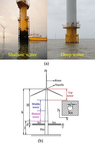
According to the field investigation report and the design documents for the wind turbine, Table 1 provides the basic design conditions and parameters.

Table 1. Specifications of the wind turbine.

Item/parameter	Value
Rated power (MW)	3
Rotor orientation, configuration	Clockwise, upwind, three blades
Cut-in, rated, cut-out wind speeds (m/s)	3.0, 11.5, 25
Cut-in, rated rotor speeds (r.p.m.)	6.58, 11.1
Ambient temperature (°C)	−30–+40
Rotor, hub diameters (m)	115, 5.767
Hub height (m)	80
Blade length (m)	55
Rated rotation speed of rotor (r·min^−1)	13.2
Rated torque (kN·m)	2426
Single blade mass (kg)	13,500
Hub mass (kg)	27,783
Nacelle mass (kg)	131,427
Design life (years)	20

The wind turbine tower is constructed as a cylinder in which both the cross section and the wall thicknesses constantly vary. Q345C steel was used to build the tower and the pile above the ground. The outer diameter and the wall thickness of the structure are in the ranges 3.1–4.5 m and 18–50 mm, respectively. The materials have a Poisson ratio of γ = 0.3, a yield strength of σ_y = 345 MPa and an elasticity modulus of E = 2.06 × 10¹¹ Pa. The stress–strain relationship of the steel is a bilinear model suggested by Japanese specifications (Japan Road Association, 2002). Accordingly, the elasticity modulus is E/100. The pile–soil interactions are simulated using a spring and the p–y curve approach. The models of the tower and the pile are established using a four-node shell element, and those of the hub and nacelle using an eight-node solid element. As for the blade, its model is shown as a four-node shell element. The blades, nacelle and hub are connected to the tower via rigid couplings. The numerical model is illustrated in Figure 4.

Figure 4. Numerical model of the structure: (a) local zoomed-in view of the numerical model; (b) numerical model.

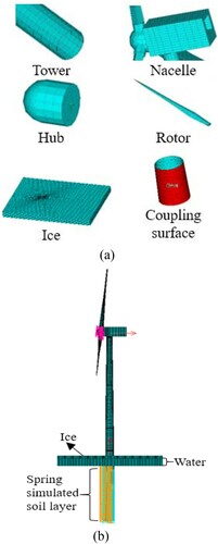
Table 2 provides physical and mechanical parameters of the hub, blade, nacelle and monopile obtained from the design manual and used in our established numerical model.

Table 2. Model parameters of the wind turbine used in this analysis.

Component	Density (kg/m^3)	Poisson ratio	Elasticity modulus (MPa)	Yield stress (MPa)	Mass (kg)
Nacelle	2460	0.22	2.5 × 10^4	378	27,783
Blade	1813	0.25	2.43 × 10^5	580	13,500
Hub	7419	0.30	1.82 × 10^5	350	131,427
Monopile	7850	0.28	2.06 × 10^5	345	307,451
Tower	7850	0.28	2.06 × 10^5	345	227,468

Through field monitoring, we found that the largest annual ice thickness can reach 0.7 m. The physical-mechanical parameters used in the analysis were obtained from indoor experiments and are listed in Table 3.

Table 3. Ice parameters used in this study.

Physical quantity	Density (kg/m^3)	Shear modulus (GPa)	Yield stress (MPa)	Plastic hardening modulus (GPa)	Bulk Modulus (GPa)	Plastic failure strain (%)	Truncation pressure (MPa)
Value	900	2.4	2.2	4.5	5.4	0.38	−4.0

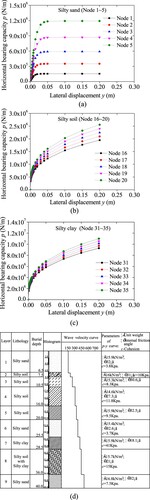
The soil sediments were investigated by drilling 40 m deep boreholes. They consist of nine layers, which are composed of silty sand (6.5 m), silty soil (1.0 m), silty soil (3.0 m), silty soil (5.5 m), silty soil (4.0 m), silty sand (5.5 m), silty clay (3.0 m), silty clay (7.5 m) and silty sand (4.0 m) from bottom to top. The parameters of the soil were obtained through laboratory tests and in situ tests. The soil layers and parameters were obtained in our related research (Huang et al., 2019), and the borehole diagram is shown in Figure 5. Here, the p–y curve method (Zhang & Andersen, 2017) is used for simulating pile–soil interactions. The segmentation is taken 1 m, and a spring is set at each node. Therefore, there are 41 nodes in the pile below ground. The p–y curves of a few representative soil layers (silty sand, silty soil and silty clay) below ground are listed, as shown in Figure 5.

Figure 5. Curves of p–y for simulating pile–soil interplay: (a) silty sand 1–5; (b) silty soil 16–20; (c) silty clay 31–35; (d) borehole diagram.

The main fault in this region is the Subei coastal fault, and it has been recorded that totally 57 destructive earthquakes have occurred here. The highest ever earthquake magnitude recorded was at magnitude 8. According to the Chinese code (GB50135-2019, 2019), for more important structures, the anti-seismic grade shall be one degree of magnitude higher. Consequently, the wind turbine should be built at an anti-seismic grade of 9, with a peak acceleration of 4 m/s² in the seismic design. To eliminate random effects of the seismic wave, less than three seismic waves are used. However, the selection of the types of seismic wave is not specified in the code. In accordance with the standard (Japan Road Association, 2002), the far-field earthquakes (referred to as T1) and near-field earthquakes (referred to as T2) are selected, and the site type is II. Figure 6 and Table 4 separately show time histories for accelerations of the seismic waves and basic characteristics of the seismic records.

Figure 6. Seismic waves: (a) time histories; (b) response spectra.

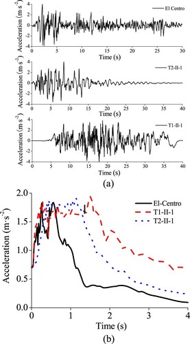
Table 4. Parameters for three types of seismic wave.

No.	Earthquake	Magnitude	Epicentral distance (km)	Location	Peak acceleration (cm/s^2)
T1-II-1	Hotan earthquake in 1968	7.5	100	Foundation of plate island bridge	362.617
T2-II-1	Kobe earthquake in 1995	7.2	11	Takatori station	686.831
El Centro	Imperial Valley earthquake in 1940	7.0	9	El Centro, Southern California	341.70

The wind pressure generated by the wind load has a certain influence on the structure (Mou et al., 2017); therefore, wind loads are applied to the wind turbine according to the code (GB50135-2019, 2019): (13) $\begin{array}{r}{\omega }_{ki}={\text{β}}_{zi}{\mu }_s{\mu }_{zBi}{\omega }_0\end{array}$(13) where ${\omega }_{ki}$ represents the standard value for the unit projected area of the wind turbine at height z and ${\omega }_0$ represents basic wind pressure, being 0.7 kN/m² for a return period of 50 years following the code (GB50135-2019, 2019). ${\mu }_{zBi}$, ${\mu }_s$ and ${\text{β}}_{zi}$ are the variation factor of height for wind pressure at height z, shape factor and wind vibration factor at height z, respectively.

2.3. Effect analysis of the monopile foundation

When designing a wind turbine, the monopile foundation is important to the total support of the structure. During the seismic design of a wind turbine, displacement and acceleration are important reference designators to determine the structure’s service performance under the existing specifications (Japan Society of Civil Engineering, 2007). Therefore, when determining the effect of the monopile foundation on the support structures, the relative displacement and acceleration are investigated when the monopile foundation is and is not considered (Figure 7).

Figure 7. Displacement and acceleration considering and not considering the monopile foundation: (a) displacement; (b) acceleration.

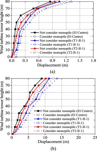
Figure 7 shows that the displacement and acceleration of the wind turbine relative to the ground are greater when considering the influence of the monopile foundation than when not considering the influence of the monopile foundation. The displacement increases by a maximum of 30.6%, except for at the tower’s bottom, while the acceleration increases by a maximum of 28.8%. The far-field earthquake significantly affects the displacement and acceleration. Consequently, the effect of the monopile foundation on the wind turbine cannot be neglected under strong earthquake activity.

2.4. Modal analysis of the wind turbine

Modal analysis is a method of studying the dynamic characteristics of a structure, and modal analysis can determine natural vibration frequencies and mode shapes at the natural vibration frequencies of the structure. The mode shapes can be used to indicate the most likely deformation of the wind turbine, and they can also reflect the deformation characteristics of the different parts, such as which parts are rigid and which parts are soft. The seismic deformation of the wind turbine is a superposition of the different modes, and the first two mode shapes are the most likely deformations of the wind turbine. Therefore, modal analysis is a critical step when analysing the seismic dynamics of wind turbines. First, we conduct modal analysis of the structure with and without sea ice. The order-1 and order-2 mode shapes of the wind turbine are illustrated in Figure 8, and their periods are listed in Table 5.

Figure 8. The order-1 and order-2 mode shapes of the wind turbine: (a) no ice; (b) ice of thickness

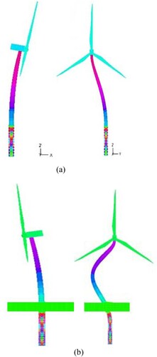
Table 5. Periods of the first two mode shapes of the structure.

	No ice			Ice thickness of 0.7 m
Category	Order-1 mode	Order-2 mode		Order-1 mode	Order-2 mode
Period (s)	0.82	0.41		0.38	0.27

As shown in Table 5 and Figure 8, the first two mode periods (order-1 and order-2) are 0.82 and 0.41 s, suggesting that the wind turbine is a structure with long periods in the absence of ice influences. The two mode periods decrease by 53.7% and 34.1% when the influence of the ice is considered. When the influence of the ice is absent, the vibration modes are bending deformation; while they are a combination of bending and torsion deformation when the influence of the ice is considered. This demonstrates that the existence of ice is disadvantageous to the seismic performance of the structure, and it will produce a large torsion displacement. Therefore, it is determined that the influence of ice upon the dynamic characteristics of the structure cannot be ignored.

3. Validation of the numerical model

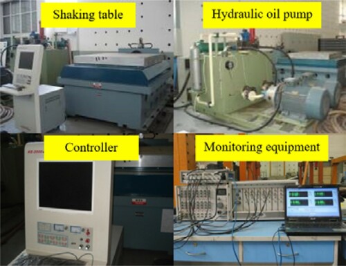
Seismic simulation tests are carried out for proving the reasonableness of the established numerical model, followed by the creation of two simplified wind turbine test models, which are used to test the earthquake response of the structure when there is sea ice and when there is none. The size of the shaking table is 1.5 m × 1.5 m, on which the maximum working load of 500 kN can be applied, and the peak acceleration in the horizontal direction is 2.0 g (where g is the gravitational acceleration of the Earth). The shaking table can be applied at frequencies in the range 0.1–50 Hz, and it can simulate different types of seismic wave. The shaking table equipment and monitoring equipment used in this study are shown in Figure 9.

Figure 9. Shaking table (ES-15).

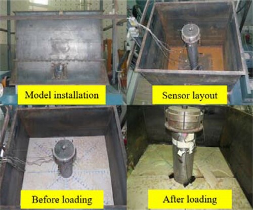
3.1. Test model

In the test, we focus on verifying the accuracy of the simple numerical method used to simulate the ice–water–wind turbine interactions, so the mass of the superstructures (nacelle, rotor and hub) are simplified to a block mass at the top of the test model. A water tank with dimensions of 2.0 m × 1.5 m × 1.5 m (length × width × height) is fixed to the table for containing water and ice. The wind turbine is 80 m high, and the mass of its superstructure is 199,710 kg. Limited by the dimensions of the equipment, a similarity coefficient of ${\lambda }_l$ = 1:50 is used. As shown in Figure 10, the model is 1.6 m high, and its base is fixed to the bottom of the tank.

Figure 10. Test models.

Before determining the similarity ratio of the model test, we make the following assumptions.

1. The same law is followed by the ice, water and wind turbine.

2. The superstructure of the wind turbine is reduced to mass blocks to meet the gravity effect and inertial force effect of the wind turbine.

3. The parameters of dynamic loads applied to the model are within allowable ranges of the equipment.

Before conducting the shaking table test, a similar relationship between the wind turbine and the test model is determined. The inertial force, resilience and gravitational force are simulated in the test; therefore, the requirements for the density and elasticity modulus of the material are relatively high. In our test, the elastic force–gravity similarity law is used to ensure the Cauchy constants, with consistent Froude constants, are shared by the wind turbine and the test model. The method of calculating the similarity coefficient is as follows. According to the Buckingham theorem (Louis, 1957), there are six dynamic equilibrium equations for a structure in a three-dimensional space, and we take the dynamic equilibrium equation in the x-axis direction as an example (Equation 14): (14) $\begin{array}{r}\frac{\mathrm{\partial }{\sigma }_x}{\mathrm{\partial }x}+\frac{\mathrm{\partial }{\tau }_{xy}}{\mathrm{\partial }y}+\frac{\mathrm{\partial }{\tau }_{xz}}{\mathrm{\partial }z}+{\gamma }_x=\rho \frac{{\mathrm{\partial }}^{2}u}{\mathrm{\partial }{t}^2}\end{array}$(14) where ${\sigma }_x$, ${\tau }_{xy}$ and $u$ are the stress, shear stress and displacement, respectively, and $\gamma$ is the unit weight.

By integrating Equation (14), Equation (15) can be set up: (15) $\begin{array}{rl}& 0.5t^2\left(\frac{\mathrm{\partial }{\sigma }_x}{\mathrm{\partial }x}+\frac{\mathrm{\partial }{\tau }_{xy}}{\mathrm{\partial }y}+\frac{\mathrm{\partial }{\tau }_{xz}}{\mathrm{\partial }z}+{\gamma }_x\right)\\ & +Ct+D=\rho u\left(C=D=0\right)\end{array}$(15) The similarity constant is substituted into Equation (15) to obtain the equilibrium equation for the test model, which is expressed by Equations (16) and (17): (16) $\begin{array}{rl}& 0.5t^{\mathrm{\prime }2}{{\lambda }_t}^2\left[\frac{{\lambda }_{\sigma }}{\lambda L}\left(\frac{\mathrm{\partial }{\sigma }_{x^{\mathrm{\prime }}}}{\mathrm{\partial }{x}^{\mathrm{\prime }}}+\frac{\mathrm{\partial }{\tau }_{x{y}^{\mathrm{\prime }}}}{\mathrm{\partial }{y}^{\mathrm{\prime }}}+\frac{\mathrm{\partial }{\tau }_{x{z}^{\mathrm{\prime }}}}{\mathrm{\partial }{z}^{\mathrm{\prime }}}\right)+{\lambda }_{\gamma }{\gamma }_{x^{\mathrm{\prime }}}\right]\\ & ={\lambda }_{\rho }{\lambda }_u{\rho }^{\mathrm{\prime }}{u}^{\mathrm{\prime }}\end{array}$(16) (17) $\begin{array}{rl}& 0.5t^{\mathrm{\prime }2}\left[\left(\frac{\mathrm{\partial }{\sigma }_{x^{\mathrm{\prime }}}}{\mathrm{\partial }{x}^{\mathrm{\prime }}}+\frac{\mathrm{\partial }{\tau }_{x{y}^{\mathrm{\prime }}}}{\mathrm{\partial }{y}^{\mathrm{\prime }}}+\frac{\mathrm{\partial }{\tau }_{x{z}^{\mathrm{\prime }}}}{\mathrm{\partial }{z}^{\mathrm{\prime }}}\right)+\frac{{\lambda }_{\gamma }{\lambda }_l}{{\lambda }_{\sigma }}{\gamma }_{x^{\mathrm{\prime }}}\right]\\ & =\frac{{\lambda }_{\rho }{\lambda }_u{\lambda }_L}{{\mathrm{\partial }}_{\tau }^2{\lambda }_{\sigma }}{\rho }^{\mathrm{\prime }}{u}^{\mathrm{\prime }}\end{array}$(17) where ${\lambda }_{\gamma }$, ${\lambda }_t$, ${\lambda }_{\sigma }$ and ${\lambda }_l$ are similarity coefficients of the unit weight, time, stress and length, respectively.

The equilibrium equation for the prototype structure is as follows. (18) $\begin{array}{r}0.5t^{\mathrm{\prime }2}\left[\left(\frac{\mathrm{\partial }{\sigma }_{x^{\mathrm{\prime }}}}{\mathrm{\partial }{x}^{\mathrm{\prime }}}+\frac{\mathrm{\partial }{\tau }_{x{y}^{\mathrm{\prime }}}}{\mathrm{\partial }{y}^{\mathrm{\prime }}}+\frac{\mathrm{\partial }{\tau }_{x{z}^{\mathrm{\prime }}}}{\mathrm{\partial }{z}^{\mathrm{\prime }}}\right)+{\gamma }_{x^{\mathrm{\prime }}}\right]={\rho }^{\mathrm{\prime }}{u}^{\mathrm{\prime }}\end{array}$(18) By comparing Equations (17) and (18), the similarity coefficients can be obtained (Table 6).

Table 6. Similarity coefficients.

Items Geometric relationship	Physical quantities Length	Relationships Controlled variable ${\lambda }_l$	Similarity coefficients 0.02
	Displacement	${\lambda }_u$ = ${\lambda }_l$	0.02
	Area	${\lambda }_A={\lambda }_l^2$	4 × 10^−4
Material relationship	Density	Controlled variable ${\lambda }_{\rho }$	1
	Poisson’s ratio	$\mu$	1.5
	Elasticity modulus	${\lambda }_E=\frac{{\lambda }_{\gamma }{\lambda }_l}{{\lambda }_{ϵ}}$	0.02
	Stress	${\lambda }_{\sigma }$ = ${\lambda }_E$	0.02
	Strain	${\lambda }_{ϵ}$ = ${\lambda }_{\sigma }$/${\lambda }_E$	1
Dynamic relationship	Time	${\lambda }_t={\lambda }_l\sqrt{{\lambda }_{\rho }/{\lambda }_E}$	0.14
	Frequency	${\lambda }_f=1/{\lambda }_t$	7.14
	Velocity	${\lambda }_V={\lambda }_l/{\lambda }_t$	0.14
	Acceleration	${\lambda }_a=\frac{{\lambda }_l}{{{\lambda }_t}^2}$	1.02
Load relationship	Bending moment	${\lambda }_M$ = ${\lambda }_E{\lambda }_l^3$	1.6 × 10^−7
	Inertial force	${\lambda }_F$ = ${\lambda }_{\rho }{\lambda }_l^3{\lambda }_a$	8.16 × 10^−6

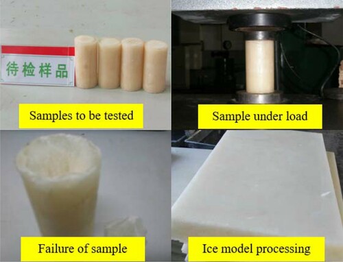
3.2. Selecting ice materials

In this study, we use paraffin to simulate the sea ice load, and the compressive strength is an important mechanical property of the ice under earthquake activity. Thus, we make different paraffin samples to find samples with compression strengths closest to that of ice. The small specimen approach is used to test the compressive strength (Equation 19): (19) $\begin{array}{r}{\sigma }_{cu}=\frac{P_f}{\pi r^2}\end{array}$(19) where $r$ is the sample’s radius, $P_f$ is the compression load when the sample is damaged, and ${\sigma }_{cu}$ is the compression strength.

During the compression experiments, the compression load is applied step by step until the sample is damaged (Figure 11). The ultimate compression loads of the four samples are 1078.83 kPa (Sample #1), 1122.79 kPa (Sample #2), 1273.51 kPa (Sample #3) and 1223.48 kPa (Sample #4). The compressive strength of the ice in our study is 1310.0 kPa. Therefore, Sample #3 meets our requirements.

Figure 11. Compression experiment and ice model.

Because the test requirement for the elasticity modulus of the material is relatively high in our shaking table test, we monitor the axial displacement using a compression load increment of 0.2 kN to calculate the elasticity moduli of the four samples. According to Hooke’s law, we obtain their stress–strain curves (Figure 12).

Figure 12. Stress–strain curves.

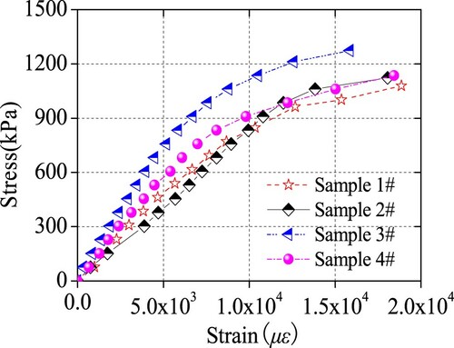
As shown in Figure 12, the paraffin samples used to simulate the ice are in the elastic stage at the beginning of compression. Slopes of stress–strain curves in the elastic deformation zone are used to calculate the elasticity modulus. Table 7 shows the calculation results.

Table 7. Elasticity moduli of the various samples.

	Sample #1	Sample #2	Sample #3	Sample #4
Elasticity modulus (MPa)	100.54	84.66	156.94	117.65

According to the similarity relationship (Table 6), the elastic modulus of the ice model is 129.6 MPa, which is close to those of Samples #3 and #4 (Table 7). Considering that the compression strength of the ice is close to that of Sample #3, paraffin Sample #3 is more in line with the test requirements.

3.3. Test schemes

In the shaking table tests, seven sensors are used to monitor the model, including five acceleration sensors and two displacement sensors. The parameter information and sensor layout are shown in Table 8.

Table 8. Sensor assignment.

Sensors	Models	Serial number	Range
Acceleration sensors	LC0701	A1, A2, A3, A4, A5	Recording acceleration (range: 0.01–20 m/s^2)
Displacement sensors	SW-1	S1, S2	Recording displacement (range: ± 100 mm)

3.4. Test results analysis

To determine the natural frequencies of the experimental model when there is ice and when there is none, we perform hammer decay model tests the sine wave sweep tests. The test results are displayed in Figure 13.

Figure 13. Fourier spectra: (a) affected by ice; and (b) not affected by ice.

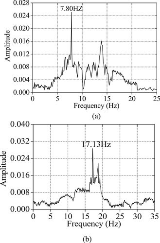
As can be seen in Figure 13, there are multiple peaks in the Fourier spectra. This shows that the model has resonance phenomena at multiple points. The frequency corresponding to the first peak is the model’s natural frequency. With no ice to exert influences, the natural frequency of the model is

 7.80 Hz, with the natural vibration period, the reciprocal of the frequency, being 0.128 s. Based on the similarity coefficient transformation, the period is 0.92 s, while the first-order period of the wind turbine is calculated to be 0.82 s using our established simplified numerical model (Table 9), and the error is 12%. Similarly, with the influence of the ice, the period obtained from the test is 0.42 s, while the first-order period of the wind turbine is calculated to be 0.38 s using our established simplified numerical model, and the error is 11%. There are numerous reasons for these errors, including the simplification of the superstructure to a lump mass, the attenuation of the conductor, and the boundary reflection of the seismic waves. However, the difference is within the error range for engineering structural design.

Table 9. Peak displacement and acceleration comparison: test and calculation results.

	Peak displacement (m)			Peak acceleration (m/s^2)
Seismic waves	Test results	Our established method	Rdis (%)	Test results	Our established method	Racc (%)
El-Centro	0.0040	0.0038	5.0	1.38	1.25	9.4
T1-II-1	0.0075	0.0073	2.7	1.72	1.59	7.6
T2-II-1	0.0034	0.0032	5.9	1.52	1.37	9.8

For the purpose of comparing the seismic dynamic responses of the test model with those of the simplified numerical model established in the research, we monitor the displacement and acceleration of the model at different heights (Table 9). The peak acceleration is set to 1 m/s². The results of the comparison are shown in Figures 14 and 15.

Figure 14. Peak displacement comparison: (a) El Centro; (b) T1-II-1; (c) T2-II-1.

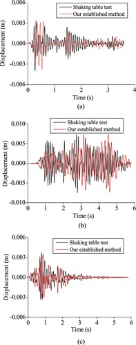
Figure 15. Peak acceleration comparison: (a) El Centro; (b) T1-II-1; and (c) T2-II-1.

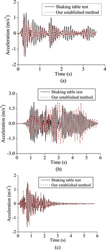
In Figures 14 and 15, the tested peak displacement and acceleration are in good agreement with the results calculated using the established simplified numerical model, with a maximum deviation of about 9.8%. However, the results for displacement and acceleration obtained by calculation are greater than the test results. This phenomenon is mainly due to the simplification of the superstructure to a lump mass, the attenuation of the conductor and the boundary reflection of the seismic waves. In addition, the calculated values of the acceleration time history and displacement time history at the model top coincide with the test results under earthquake action. Consequently, the consistency between the calculated results and the test results demonstrates the accuracy and reliability of the established simplified numerical model. Additionally, comparisons are performed for the calculated peak displacements and peak accelerations at points up the height (Figure 16).

Figure 16. Peak displacements and accelerations over the height of the model: (a) displacements; (b) accelerations.

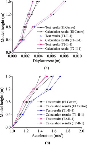
As Figure 16 shows, results of the test model under earthquake activities conform well to results calculated by the proposed approach. Only slight deviations are observed under certain conditions. The difference is found to be as large as 10.20% in terms of the peak acceleration when subjected to El Centro. The maximum error of the maximum value of the displacement is 13.45% when subjected to T1-II-1. Basically, the calculated results of the established simplified numerical model are consistent with the experimental results, further validating the accuracy and reliability of the established simplified numerical model.

4. Seismic behavior of the structure under ice influences

In general, influences of ice on wind turbines in terms of the seismic design are mainly reflected in the ice thickness and ice size; therefore, we mainly investigate the influences of the ice thickness and the ice boundary range upon the seismic performance of the structure. In the numerical analysis, the boundary conditions for sea ice first need to be determined. If the ice boundary range is not set properly, there will be a large error in the calculation results. Consequently, first we explore the influences of the boundary range of the ice on the seismic behavior of the structure.

4.1. Effect of ice boundary range

This study defines the ice boundary range as the ratio of the horizontally-projected area of ice around the wind turbine to the horizontal cross-sectional area of the tower, expressed as R. The ice is 0.7 m thick and R is set to 0, 10, 20, 30, 40, 50, 60, 70, 80, 90 and 100. In addition, we take the rate of change to reflect influences of the boundary range of sea ice upon the maximum seismic response of the structure. (20) $\begin{array}{r}\text{Change}\text{rate}=\frac{M_{\text{ice}}-M_o}{M_o}\end{array}$(20) where $M_{\text{ice}}$ and $M_o$ are the maximum responses of the wind turbine in cases with and without ice, respectively.

The internal forces at the tower bottom represent the structural resistance to external forces under horizontal external forces, so they are critical to the seismic performance of the structure. Therefore, we study the influences of different boundary ranges of sea ice on the internal forces at the bottom of the structure (Figure 17).

Figure 17. Rates of change of bending moment and shear force: (a) bending moment; (b) shear force.

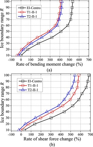
As shown in Figure 17, as the boundary range of ice enlarges, the rates of change of both the shear force and bending moment at the structural bottom gradually increase. When the ice boundary range reaches a certain value, its influences on the bending moment and shear force gradually stabilize. When R is less than 60, the internal force increases linearly. The rate of change of the bending moment reaches 489%, and that of the shear force reaches 582%. When R is greater than 60, the influences of the ice boundary range on the bending moment and shear force gradually decrease. These results suggest that, when R is 60, the influences of the ice boundary range on the internal forces in the seismic design of such structures built in icy water should have attention paid to them. The values of the internal force increase sharply with the enlarging size of sea ice, which is because ice with a certain mass vibrates along the wind turbine, which can increase the horizontal thrust of the wind turbine. According to the principle of structural dynamics, the inertial forces of the wind turbine will increase with growing mass of the wind turbine. Furthermore, the vibration period of the structure increases under the influence of the ice (Figure 8(b)), which causes the natural period of the wind turbine to become close to the predominant period of the response spectra of the seismic waves. Resonance occurs when the wind turbine’s period is close to the predominant period. Therefore, the bending moment and shear force as internal forces of the structure increase as the size of the sea ice increases.

In seismic code in China and abroad, the earthquake-induced hydrodynamic pressure cannot be ignored during the seismic design of wind turbines. To analyse the influences of the ice boundary range on the hydrodynamic pressure, we investigate the distribution of the hydrodynamic pressure at points up the height of the structure under various seismic excitation inputs for a water depth of 15 m (Figure 18).

Figure 18. Hydrodynamic pressure under the effects of various boundary ranges of sea ice: (a) El Centro; (b) T1-II-1; (c) T2-II-1.

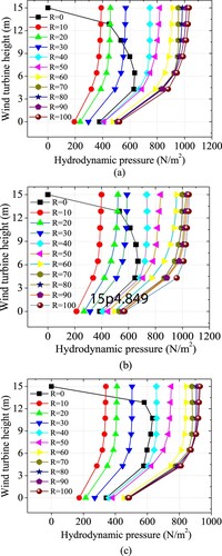
As Figure 18 shows, the hydrodynamic pressure at points up the height is parabolically distributed in the absence of sea ice, showing an increase at first and then a decreasing trend. The maximum value appears at two-fifths of the water depth. By contrast, under the influence of sea ice, the hydrodynamic pressure increases linearly until two-fifths of the water depth, at which point the hydrodynamic pressure increases slowly. As the ice boundary range increases, the hydrodynamic pressure increases. The influence amplitude of the ice boundary range on the hydrodynamic pressure decreases when R reaches 60. Taking the hydrodynamic pressure at an R-value of 10 as the benchmark, when R is 100, the maximum hydrodynamic pressures under the three earthquake excitations increase by 129.0%, 97.1% and 117.0%, respectively. When R is 60, the maximum hydrodynamic pressures under the three input earthquake excitations separately increase by 110.0%, 79.2% and 99.5%, respectively. We find that the hydrodynamic pressure at the water surface is zero when the effect of the ice is not considered; however, the hydrodynamic pressure is large at the water surface when the effect of the ice is considered. The main reason for this is that the dynamic interaction between the water and ice amplifies the hydrodynamic pressure (Kobayashi, 2002; Jia & Han, 2011). The fluid–solid coupling between the water and ice under earthquake activity can induce friction on the ice surface and surface tension on the water that causes the water to vibrate violently, thus forming a large hydrodynamic pressure. The hydrodynamic pressure is affected more greatly by El Centro compared with the other two seismic excitation inputs. The result demonstrates that sea ice not only has a large effect on the hydrodynamic pressure’s amplitude but also changes its distribution law. In particular, when R is less than 60, the ice boundary range significantly influences the hydrodynamic pressure.

The influences of the ice boundary range upon the structure’s acceleration and displacement are also important indexes. Taking the El Centro seismic wave as an example, Figure 19 illustrates the acceleration and displacement relative to the ground under different ice boundary ranges and water of 15 m depth.

Figure 19. Displacement and acceleration under the various ice boundary ranges: (a) displacement; (b) acceleration.

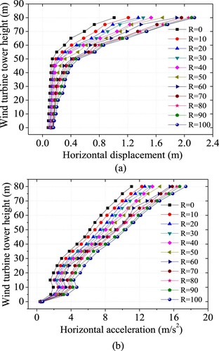
As can be seen from Figure 19, the displacement and acceleration values of the structure are much more greatly influenced by the sea ice than the values without the ice influence. Moreover, as the ice boundary range increases, the maximum displacement and acceleration both increase up the wind turbine’s height. There is a large increase in the amplitude when R is less than 60, but the increase in the amplitude decreases when R is greater than 60. When there is sea ice, the structure exhibits increasing displacement with increases in the ice boundary range, and the largest rate of change is 85%. Simultaneously, the acceleration also increases. There is an inflection point at the ice–wind turbine contact. When affected by sea ice, the acceleration changes more significantly with increasing height, with a maximum rate of change of 94%. Because of the ice–structure interaction, sea ice vibrates with the structure, and the structural vibration is enhanced under the dynamic action of the earthquake. Therefore, the ice–structure interactions increase the acceleration and deformation. As the boundary size of the ice increases, the mass of ice increases, and the natural period of the wind turbine increases under the influence of ice. If the period of the structure (affected by the ice) is close to the predominant period of the seismic response spectrum (Figure 6(b)), the acceleration and displacement of the wind turbine are further magnified under earthquake activity.

4.2. Influences of ice thickness

The thickness of the ice varies over the seasons and temperatures. This necessitates research on the influence of sea ice with different thicknesses on the seismic performance of such structures. In the following calculations, the water depth is set to 15 m, and five conditions are considered by setting the ice thickness to 0.3, 0.4, 0.5, 0.6 and 0.7 m. As mentioned above, El Centro seismic excitation influences how the wind turbine responds dynamically to seismic activities. Thus, we analyse the structure’s seismic behavior under the seismic excitation inputs of El Centro. Thereby, the maximum hydrodynamic pressure distributed over the height of the structure is extracted (Figure 20).

Figure 20. Distribution of the hydrodynamic pressure: (a) hydrodynamic pressure; (b) change rate.

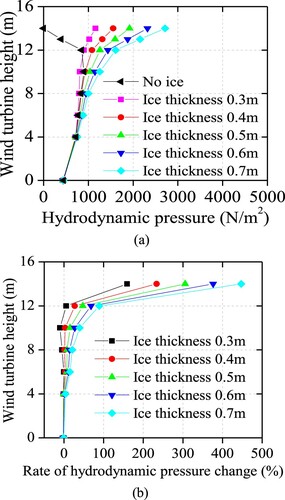
As can be seen from Figure 20, under seismic loads, there is a significant difference in the distribution of the hydrodynamic pressure, and the distribution exhibits the same trend as in Figure 18. Two-fifths of the water depth is a turning point in the change in the hydrodynamic pressure. Under the influence of sea ice, the hydrodynamic pressure shows a sharply increasing amplitude when the water depth is below the turning point. Without the ice’s influence, the hydrodynamic pressure exhibits a transition in the change trend from increasing to decreasing when the water depth is below the turning point. Moreover, with growing sea ice thickness, the hydrodynamic pressure increases and so does the influence coefficient thereof. The reason for this is that the increase in the thickness of the ice increases the ice’s mass, and the vibration of the ice is intensified by the earthquake activity, which makes the ice’s surface produce greater tension on the surface of the water. The increase in the water’s surface tension induces the water to vibrate violently, and this phenomenon increases the hydrodynamic pressure. Therefore, under seismic loads, the ice not only changes the amplitude value but also distribution forms of hydrodynamic pressure.

Shear force and bending moment at the tower bottom reflect structural resistance to external forces under the effect of a horizontal external load, so they are important factors when analysing the seismic behavior of such structures. Therefore, taking 0.7 m thick sea ice and water of 15 m depth as an example, the time histories of the internal forces at the tower bottom affected by the El Centro earthquake are shown in Figure 21.

Figure 21. Time histories of the internal force: (a) shear force; (b) bending moment.

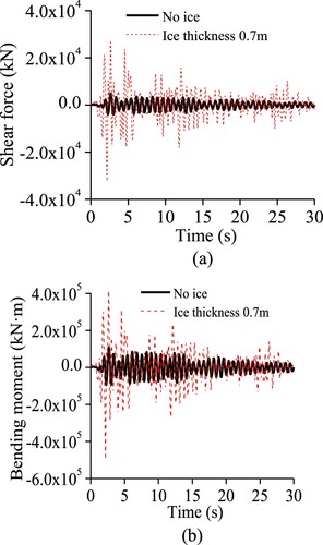
As Figure 21 shows, the changes in the time histories are significant. Under seismic activity, the amplitudes of the internal force (bending moment and shear force) changes insignificantly at the tower bottom without the influence of sea ice. By contrast, the bending moment and shear force show greatly fluctuating amplitudes when affected by the ice, which adversely impacts the seismic performance of the structure. The ice vibrates with the wind turbine, and the vibration modes of the time history are different with and without the influence of the ice. Moreover, sea ice lengthens the structure’s natural vibration period, resulting in a natural period closer to the predominant period of the response spectra of the seismic waves, making the structure more sensitive to earthquakes.

Additionally, the relative displacement serves as a key determinant for structural seismic performance. Moreover, the time histories of accelerations at the tower top represent the motions of blades, nacelle and hub. Thus, we calculate displacement and acceleration time histories as well as Fourier spectra (Figures 22 and 23).

Figure 22. Displacement time history and Fourier spectrum of the top of the tower: (a) time history; (b) Fourier spectrum.

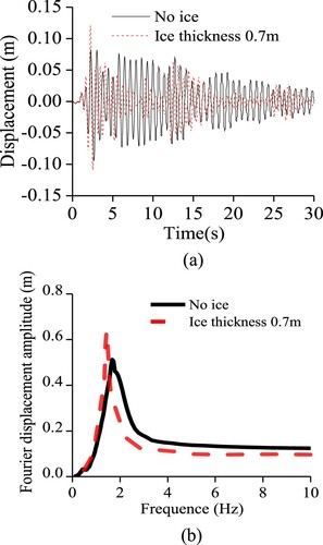
Figure 23. Acceleration time history and Fourier spectrum of the top of the tower: (a) time history; (b) Fourier spectrum.

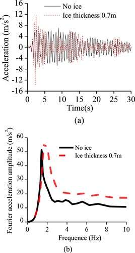
As Figure 22 depicts, the presence of ice changes the structure’s dynamic response. If sea ice is 0.7 m thick, the peak displacement at the tower top is larger than that without the ice influence, and the displacement changes at a much greater rate. As the Fourier spectra display, the displacement amplitude at the tower top is more substantially affected by the 0.7 m thick ice. Moreover, when the frequency exceeds 1.50 Hz, because of the effect of the sea ice, the horizontal displacement at the tower top has a lower Fourier amplitude than is the case without ice. This means that the tower top (when affected by sea ice) has a horizontal displacement that is sensitive to the medium-frequency and high-frequency components of the earthquake. As shown in Figure 23, like the displacement at the structure’s top, the maximum acceleration at the tower top is also greater in the presence of ice of 0.7 m thickness than that without ice. At frequencies greater than 1.5 Hz, the amplitudes of the horizontal acceleration differ significantly when affected by ice. Therefore, at the tower top, the acceleration and displacement values are affected by the ice, and they are sensitive to the earthquake’s high-frequency components.

The relationship between the bending moment and the curvature at the tower bottom is also studied (Figure 24).

Figure 24. Relationship between the bending moment and the curvature in response to various earthquake activities: (a) El Centro; (b) T1-II-1; (c) T2-II-1.

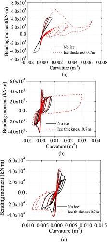
As can be seen from Figure 24, the structure bottom witnesses a closer relationship between the bending moment and the curvature with the influence of ice than without the influence of the ice. In comparison with the case with no sea ice, the inverted-S shape of the hysteretic curve is most pronounced, which is indicative of energy dissipation and a decrease in the deformation capacity of the structure. The bending moment–curvature relationship shows plastic accumulation of the structure, and it reflects the deformation characteristics and energy dissipation of the structure during the earthquake’s action. There are significant changes in the shape of the hysteresis loop that reveal that the ice greatly influences the nonlinear behavior of the wind turbine. The hysteresis loops exhibit significant deformation under the El Centro and T1-II-1 earthquakes, which shows that the wind turbine has undergone a large plastic deformation. This reduces the deformation recovery and the energy-dissipation ability of the structure, which is an important reference index for wind turbine damage under earthquake activity. Considering this, the wall thickness should be increased or stiffening ribs should be added so as to enhance the ductility performance of the structure.

The coefficient of the curvature’s ductility demands represents the deformation capacity of a structure from yield to failure. The coefficients of the curvature’s ductility demands and the maximum curvatures at the bottom of the tower under different earthquake excitations without ice and with ice of 0.7 m thickness are listed in Table 10.

Table 10. Coefficients of the curvature’s ductility demands at the bottom of the tower.

Condition	Seismic type	Curvature $\left|{\varphi }_{max}\right|\left(m^{-1}\right)$	Yield curvature ${\varphi }_y\left(m^{-1}\right)$	Coefficient of the curvature’s ductility demand $\left|{\varphi }_{max}\right|/{\varphi }_y$
No ice	El-Centro	0.00272	0.00080	3.4
	T1-II-1	0.00992	0.00080	12.4
	T2-II-1	0.00595	0.00080	7.4
Ice thickness of 0.7 m	El-Centro	0.00622	0.00080	7.8
	T1-II-1	0.03212	0.00080	40.2
	T2-II-1	0.00972	0.00080	12.2

As is shown in Table 10, under these two conditions, the maximum curvature is the largest in response to the far-field earthquake (T1-II-1), and sea ice exerts the maximum influence upon the curvature. Although the maximum curvature in response to the near-field T2-II-1 and El Centro earthquakes is also relatively large, sea ice imposes a lesser effect on the curvature compared with that of T1-II-1, a far-field earthquake. Therefore, sea ice readily causes damage to the wind turbine, and its ductility should be increased in light of these seismic design considerations. In addition, the second critical control factor for the seismic design is the residual displacement; therefore, it is necessary to investigate the impacts of the residual displacement of the top of the wind turbine imposed by the sea ice (Table 11).

Table 11. Maximum absolute displacement and residual displacement at the tower top.

	Maximum absolute displacement				Residual displacement
Seismic wave	No ice $\left|u_{max0}\right|\left(m\right)$	Ice thickness 0.7 m $\left|u_{max1}\right|\left(m\right)$	Change $R_{\text{dis}}$		No ice $\left|u_{r0}\right|\left(m\right)$	Ice thickness 0.7 m $\left|u_{r1}\right|\left(m\right)$	Change $R_{\text{res}}$
El Centro	0.152	0.248	76%		0.002	0.013	550%
T1-II-1	0.535	1.545	188%		0.020	0.195	875%
T2-II-1	0.326	0.548	68%		0.004	0.012	200%

As shown in Table 11, according to the deformation requirements in the specifications (GB50135-2019, 2019), the wind turbine is damaged under T1-II-1. In response to the T2-II-1, changes in the maximum and residual displacements at the tower top reach 68% and 200%, respectively. However, under T1-II-1 earthquake excitation, the maximum displacement and residual displacement are significantly greater than those under the other two seismic waves, which shows that sea ice insignificantly influences the absolute displacement and residual displacement under far-field earthquake activity. In addition, compared with the El Centro earthquake, the T2-II-1 earthquake excitation influences the maximum absolute displacement more greatly in the presence of sea ice; while the El Centro earthquake excitation influences the residual displacement the most. Therefore, the residual displacement and maximum absolute displacement should be taken into consideration in the seismic design of such structures.

Finally, by taking 0.7 m thick ice and 15 m deep water as an example, the influences of the ice on the internal forces over the height of the structure are studied under conditions without ice and with 0.7 m thick ice (Figure 25).

Figure 25. Influence of ice on the internal forces: (a) shear force; (b) bending moment.

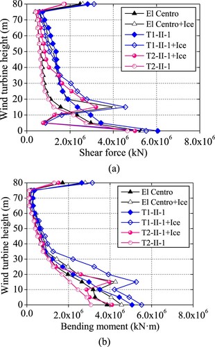
Figure 25 shows that the maximum internal forces (shear force and bending moment) with and without ice appear at the bottom of the structure; however, they exhibit different change laws with height. With ice, the contact point at the action position of the ice also generates greater internal forces, while the internal forces decrease upwards over the tower’s height. The top of the wind turbine also has a larger internal force. The reason for this is that the nacelle and rotor have a large mass, which could make the junction position between the nacelle and the tower produce a large internal force. The shear forces at the structure’s bottom and its contact point with sea ice separately grow by 18% and 95% with sea ice in response to T1-II-1, while the maximum bending moment exhibits significant increases of 20% and 73%, respectively. Owing to the increase in the thickness of the ice, the ice’s mass increases, and there is a relatively large horizontal thrust acting on the wind turbine under the earthquake activity, which increases the internal forces of the wind turbine. Therefore, in the seismic design of such structures, it is necessary to carry out anti-seismic check calculations at the bottom of the wind turbine and the contact point with the sea ice. Stiffeners at these positions also need to be added to ensure the safety of the wind turbine when it is surrounded by sea ice in the most active earthquake regions.

5. Conclusions and remarks

In this article, a simplified numerical method for wind turbine–sea ice–water interactions is developed by simplifying the fluid–solid coupling equation. On this basis, a 3D numerical model is built for studying the influences of the ice boundary range and ice thickness upon the seismic behavior of a structure on a monopile foundation subjected to near-field and far-field earthquakes. It is determined that sea ice significantly affects the distribution of hydrodynamic pressure, which exhibits a parabolic distribution over the height of the structure in the absence of sea ice, while increases linearly and then slowly in the presence of sea ice. The hydrodynamic pressure also increases as the ice boundary range and thickness increase. Prominently, the seismic behavior indexes (hydrodynamic pressure, displacement, acceleration, bending moment and shear force) show a linearly increasing trend within a certain ice boundary range, and the influence of ice upon the seismic behavior of the structure gradually decreases when the ice boundary range exceeds this value. Moreover, the sea ice–structure contact point generates a greater internal force, and as the ice thickness increases, the maximum curvature’s ductility demand on the wind turbine increases by 40.2%, and the maximum displacement and the residual displacement at the tower top increase by 188% and 10-fold, respectively, under different earthquakes excitations. This indicates that the energy-dissipation and deformation capacities of the structure are decreased by the influence of the ice, thus leading to a decreased seismic performance. When sea ice is present, the displacement and acceleration are sensitive to the high-frequency components of the seismic excitation input. The experimental results of shaking table tests demonstrate the accuracy and reliability of the proposed simplified numerical method.

This research was devised to explore the seismic performance of wind turbines with monopile foundations affected only by sea ice far from the coast. In future work, we will focus on ice near the coast, such as ice that is broken into pieces by waves and boundary constraints. Moreover, one shortcoming of this research is that it does not consider current loading, but the loading of the dynamic current, including scouring and liquefaction, affect the stability of the seabed surrounding the structure’s foundation. This will be studied in the future.

Data availability statement

Some or all data, models or code generated or used during the study are available from the corresponding author by request.

Disclosure statement

No potential conflict of interest was reported by the authors.

Additional information

Funding

This work was supported by the National Natural Science Foundation of China [grant number: 51708516]; Beijing Municipal Natural Science Foundation [grant number: 8174078]; the National Key R&D Programme of China [grant number: 2017YFC1500404]; the Young Elite Scientists Sponsorship Program by CAST [grant number: 2018QNRC001].

References

- Bouaanani, N., Paultre, P., & Proulx, J. (2004). Dynamic response of a concrete dam impounding an ice-covered reservoir: Part II. Parametric and numerical study. Canadian Journal of Civil Engineering, 31(6), 965–976. https://doi.org/https://doi.org/10.1139/l04-076
- Brown, T. G., & Morsy, U. A. (1995). Modelling of continuous crushing of ice in front of offshore structures. Canadian Journal of Civil Engineering, 22(3), 544–550. https://doi.org/https://doi.org/10.1139/l95-063
- Chen, Y., & Lian, Y. (2015). Numerical investigation of vortex dynamics in an H-rotor vertical axis wind turbine. Engineering Applications of Computational Fluid Mechanics, 9(1), 21–32. https://doi.org/https://doi.org/10.1080/19942060.2015.1004790
- Croteau, P. (1983). Dynamic interactions between floating ice and offshore structures. University of California.
- Dong, R., Li, X., & Zhou, J. (2010). Seismic analysis of offshore platform with oil storage tank including fluid-structure interaction. Journal of Ship Mechanics, 14(8), 887–893.
- GB18306-2015. (2019). Seismic ground motion parameters zonation map of China.
- GB50135-2019. (2019). Code for design of high-rising structures.
- Hacıefendioğlu, K., Bayraktar, A., & Bilici, Y. (2009). The effects of ice cover on stochastic response of concrete gravity dams to multi-support seismic excitation. Cold Regions Science and Technology, 55(3), 295–303. https://doi.org/https://doi.org/10.1016/j.coldregions.2008.08.003
- Heinonen, J., & Rissanen, S. (2017). Coupled-crushing analysis of a sea ice-wind turbine interaction – feasibility study of FAST simulation software. Ships and Offshore Structures, 12(8), 1056–1063. https://doi.org/https://doi.org/10.1080/17445302.2017.1308782
- Hendrikse, H., & Nord, T. S. (2019). Dynamic response of an offshore structure interacting with an ice floe failing in crushing. Marine Structures, 65, 271–290. https://doi.org/https://doi.org/10.1016/j.marstruc.2019.01.012
- Huang, S., Huang, M., Lyu, Y., & Xiu, L. (2021). Effect of sea ice on seismic collapse-resistance performance of wind turbine tower based on a simplified calculation model. Engineering Structures, 227, 111426. https://doi.org/https://doi.org/10.1016/j.engstruct.2020.111426
- Huang, S., Lyu, Y., & Peng, Y. (2019). Effect analysis of dynamic water pressure on dynamic response of offshore wind turbine tower. Journal of Vibroengineering, 22(1), 225–238. https://doi.org/https://doi.org/10.21595/jve.2019.20905
- ISO-19906. (2010). Arctic offshore structures standard.
- Japan Road Association. (2002). Specifications for highway bridges·Part V: Seismic design (1st ed.). Maruzen Watanabe, Ltd.
- Japan Society of Civil Engineering. (2007). Wind power gen-eration equipment support structure design guide and analysis. Series for Construction Engineering.
- Jia, L. (2010). Seismic and ice response analysis of bridge pier in deep water with the wave effect. Technology for Earthquake Disaster Prevention, 5(2), 263–269. https://doi.org/https://doi.org/10.4028/www.scientific.net/AMR.163-167.4072
- Jia, L., & Han, Y. (2011). Response analysis of bridge pier in deep water under different loads action. Earthquake Resistant Engineering and Retrofitting, 33(2), 33–36.
- Karna, T., & Turnunen, R. (1990). A straightforward technique for analyzing structural response to dynamic ice action. Proceedings of the Ninth International Conference on Offshore Mechanics and Arctic Engineering, IV, 135–142.
- Kobayashi, H. (2002, May 26-31). Evaluation of seismic load on the marine structure in ice-covered waters. Proceedings of the twelfth international offshore and polar engineering conference, Kitakyushu, Japan.
- Li, Yue, Song, Bo, & Huang, Shuai. (2011). Hydrodynamic force and its effect on the dynamic response of deep-water bridge piers in earthquake. Journal of University of Science and Technology Beijing, 33(3), 388–394.
- Louis, B. (1957). The Pi theorem of dimensional analysis. Archive for Rational Mechanics and Analysis, 1(1), 35–45. https://doi.org/https://doi.org/10.1007/BF00297994
- Meana-Fernández, A., Fernández Oro, J. M., Argüelles Díaz, K. M., Galdo-Vega, M., & Velarde-Suárez, S. (2019). Application of Richardson extrapolation method to the CFD simulation of vertical-axis wind turbines and analysis of the flow field. Engineering Applications of Computational Fluid Mechanics, 13(1), 359–376. https://doi.org/https://doi.org/10.1080/19942060.2019.1596160
- Mou, B., He, B.-J., Zhao, D.-X., & Chau, K.-w. (2017). Numerical simulation of the effects of building dimensional variation on wind pressure distribution. Engineering Applications of Computational Fluid Mechanics, 11(1), 293–309. https://doi.org/https://doi.org/10.1080/19942060.2017.1281845
- Qi, F., & Song, B. (2013). Study on the effect of sea ice on seismic response of a long-span arch bridge in icy water. China Civil Engineering Journal, 46(S1), 256–261.
- Quezada, M., Tamburrino, A., & Niño, Y. (2018). Numerical simulation of scour around circular piles due to unsteady currents and oscillatory flows. Engineering Applications of Computational Fluid Mechanics, 12(1), 354–374. https://doi.org/https://doi.org/10.1080/19942060.2018.1438924
- Ramezanizadeh, M., Alhuyi Nazari, M., Ahmadi, M. H., & Chau, K.-W. (2019). Experimental and numerical analysis of a nanofluidic thermosyphon heat exchanger. Engineering Applications of Computational Fluid Mechanics, 13(1), 40–47. https://doi.org/https://doi.org/10.1080/19942060.2018.1518272
- Risk, K., & Bridges, R. (2019). Limit state design and methodologies in ice class rules for ships and standards for Arctic offshore structures marine structures. Marine Structures, 63, 462–479. https://doi.org/https://doi.org/10.1016/j.marstruc.2017.09.005
- Shamaei, F., Bergström, M., Li, F., Taylor, R., & Kujala, P. (2020). Local pressures for ships in ice: Probabilistic analysis of full-scale line-load data. Marine Structures, 74, 102822. https://doi.org/https://doi.org/10.1016/j.marstruc.2020.102822
- Shi, Q., Tong, J., & Song, A. (2001). Characteristics of the function of ice force on vertical cylindrical piles. China Ocean Engineering, 15(3), 437–443. https://doi.org/https://doi.org/10.3321/j.issn:0890-5487.2001.03.011.0
- Wang, Y. (2014). Study of mechanism and theoretical model of ice induced vibrations of narrow structures. Dalian University of Technology.
- Withalm, M., & Hoffmann, N. P. (2010). Simulation of full-scale ice–structure-interaction by an extended Matlock-model. Cold Regions Science and Technology, 60(2), 130–136. https://doi.org/https://doi.org/10.1016/j.coldregions.2009.09.006
- Xiangjun, B., Tuomo, K., Qianjin, Y., & Yan, Q. (2006). A random ice force model for narrow conical structures. Cold Regions Science and Technology, 45(3), 148–157. https://doi.org/https://doi.org/10.1016/j.coldregions.2006.05.008
- Yu, Z., Lu, W., van den Berg, M., Amdahl, J., & Løsetcd, S. (2021). Glacial ice impacts: Part II: Damage assessment and ice-structure interactions in accidental limit states (ALS). Marine Structures, 75(75), 102889. https://doi.org/https://doi.org/10.1016/j.marstruc.2020.102889
- Yue, Q., Bi, X., Yu, X., & Shi, Z. (2003). Ice-induced vibration and ice force function of conical structure. China Civil Engineering Journal, 36(2), 16–19. https://doi.org/https://doi.org/10.1007/s11769-003-0044-1
- Zhang, Y., & Andersen, K. H. (2017). Scaling of lateral pile p-y response in clay from laboratory stress-strain curves. Marine Structures, 53, 124–135. https://doi.org/https://doi.org/10.1016/j.marstruc.2017.02.002
- Zhou, M., & Zhang, Y. (2009). Dynamic characteristic analysis of elastic fluid-filled tank considering liquid sloshing. Journal of China University of Petroleum, 33(5), 114–118.
- Zhu, B., Sun, C., & Jahangiri, V. (2021). Characterizing and mitigating ice-induced vibration of monopile offshore wind turbines. Ocean Engineering, 219, 108406. https://doi.org/https://doi.org/10.1016/j.oceaneng.2020.108406