Introducing an evolutionary-decomposition model for prediction of municipal solid waste flow: application of intrinsic time-scale decomposition algorithm

Abstract

Owing to the importance of municipal waste as a determining factor in waste management, developing data-driven models in waste generation data is essential. In the current study, solid waste generation is taken as the function of several parameters, namely month, rainfall, maximum temperature, average temperature, population, household size, educated man, educated women, and income. Two different stand-alone computational models, namely, gene expression programming and optimally pruned extreme machine learning techniques, are used in this study to establish their reliability in municipal solid waste generation forecasting, followed by Mallow’s coefficient feature selection method. The lowest Mallow’s coefficient defines the optimal parameters in solid waste generation forecasting. The novel hybrid models of intrinsic time-scale decomposition-gene expression programming and intrinsic time-scale decomposition- optimally pruned extreme machine learning methods based on Monte-Carlo resampling are employed, and an empirical equation is presented for solid waste generation prediction. For examining the reliability of these models, five statistical criteria, namely coefficient of determination, root mean square error, percent mean absolute relative error, uncertainty at 95% and Willmott’s index of agreement, are implemented. Considering Willmott’s index, the Monte Carlo-intrinsic time-scale decomposition-gene expression programming model attains the closest value (0.957) to the ideal value in the training stage and 0.877 in the testing stage. The hybrid ensemble model of intrinsic time-Scale decomposition-gene expression programming presented lower values of root mean square error (12.279) and percent mean absolute relative error (4.310) in the training phase and in the testing, phase compared to gene expression programming with (12.194) and (5.195), respectively. Overall, the prediction results of the hybrid model of intrinsic time-scale decomposition-gene expression programming using Monte-Carlo resampling technique agrees well with the observed solid waste generation data.

KEYWORDS:

• Waste management
• artificial intelligence
• intrinsic time-scale decomposition (ITD) algorithm
• gene expression programming
• machine learning
• circular economy (CE)

Abbreviations

ANFIS	=	Adaptive Neuro-Fuzzy Inference System
AIC	=	Akaike Information Criterion
AI	=	Artificial Intelligence
ANN	=	Artificial Neural Network
EDU	=	Average Education per Household
Tave	=	Average Temperature
BIC	=	Bayesian Information Criteria
R2	=	Coefficient of Determination
CWT	=	Continuous Wavelet Transform
DDMs	=	Data-Driven Models
DWT	=	Discrete Wavelet Theory
EM	=	Educated Man
EW	=	Educated Women
ETs	=	Expression Trees
OPELM	=	Extreme Learning Machine
FS	=	Feature Selection
FFNN	=	Feed-Forward Neural Networks
GEP	=	Gene Expression Programming
GA-ANFIS	=	Genetic Algorithm–Adaptive Neuro-Fuzzy Inference System
GA-ANN	=	Genetic Algorithm–Artificial Neural Network
GP	=	Genetic Programming
GDP	=	Gross Domestic Product
HS	=	Household Size
ITD	=	Intrinsic Time-Scale Decomposition
KNN	=	K-Nearest Neighbors
LOO	=	Leave-One-Out
CP	=	Mallow’s Coefficient
MESA	=	Maximum Entropy Spectral Analysis
ME	=	Maximum Entropy
Tmax	=	Maximum Temperature
MT	=	Model Tree
M	=	Month
MC	=	Monte-Carlo
MARS	=	Multivariate Adaptive Regression Splines
MSWG	=	Municipal Waste Generation
MSW	=	Municipal Waste
SNIS	=	National Sanitation Information System
NH	=	Number of Residents per Household
OPELM	=	Optimally Pruned Extreme Machine Learning
PMARE	=	Percent Mean Absolute Relative Error
POP	=	Population
PCA	=	Principal Component Analysis
PRCs	=	Proper Rotation Components
RBF	=	Radial Basis Function
RF	=	Random Forest
RSW	=	Residential Waste
RMSE	=	Root Mean Square Error
SLFN	=	Single-Layer Feed-Forward Neural Network
SSA	=	Singular Spectrum Analysis
SWG	=	Solid Waste Generation
SVM	=	Support Vector Machine
TWMO	=	Tehran Waste Management Organization
U95	=	Uncertainty at 95%
WGI	=	Waste Generation Per capita Index
WMRA	=	Wavelet Multi-Resolution Analysis
WT	=	Wavelet Transform
WI	=	Willmott’s Index of Agreement

1. Introduction

Growing population and agricultural activities to provide food and water lead to massive increases in waste generation polluting the natural environment (Samal et al., 2020). These environmental issues are perceptible, especially in developing countries, because there is no particular waste management infrastructure (Arena et al., 2003). These environmental issues, namely river contamination, underprivileged agricultural practices, sanitation problems, unpleasant odor, groundwater quality pollution because of landfills seepage of leachate, dirty flies, and mosquitoes, can cause an increasing death rate year to year (El-Fadel et al., 1997; Wen et al., 2019). Waste can be classified into different categories, namely municipal (Nęcka et al., 2019), hazardous, industrial, agricultural, bio-medical, etc. In this research, the main focus is on MSW, which generally contains degradable waste (like food waste), partially degradable (like wood), and non-degradable (like plastics) (Soni et al., 2019; Tenodi et al., 2020). SWG is one of the crucial environmental challenges (Abbasi et al., 2019). It can conserve natural resources in an every-day environment, which directly affects human health (Mozhiarasi et al., 2020).

Municipal waste generation rate forecasting is one of the recent vital issues of decision-makers to develop and plan a waste management system; it can be a reliable solution in future waste management especially in populated megacities around the world (Abdulredha et al., 2020; Duan et al., 2020; Kannangara et al., 2018). Waste generation data are reported as time series in different scales such as daily, monthly, and yearly data (Liu et al., 2019). These data have quite dynamic nature (Vu et al., 2019). Due to their complexity and nonlinearity, it is essential to use a rigorous model to achieve acceptable and accurate results. As mentioned previously, different parameters are affecting the SWG models. They have high fluctuations in their amounts, therefore considering these drivers as main predictors for modeling has the highest importance (Araiza-Aguilar et al., 2020).

In recent decades, there are lots of publications about DDMs in environmental sciences such as ANN (Cevik et al., 2017), ANFIS (Kisi, Sanikhani, et al., 2017; Zamani Sabzi et al., 2017), GEP (Shiri et al., 2013), MT (Fernandez Martinez et al., 2014; Kisi & Kilic, 2015), OPELM (Şahin, 2013), MARS (Kisi, Parmar, et al., 2017), KNN (Modaresi et al., 2018; Naghibi et al., 2018), SVM (Mohammadpour et al., 2015; Mosavi et al., 2019), RF (Shiri et al., 2017; Wei, 2017), MLR (Kisi & Parmar, 2016; Mohammadi et al., 2016). Notably, there are several works that used DDMs for modeling MSW such as SVM (Abbasi & El Hanandeh, 2016; Najafzadeh & Zeinolabedini, 2019), ANN (Chhay et al., 2018; Hoque & Rahman, 2020; Oliveira et al., 2019; Soni et al., 2019), ANFIS (Abbasi & El Hanandeh, 2016; Soni et al., 2019), RF (Kumar et al., 2018), KNN (Abbasi & El Hanandeh, 2016). Some studies have performed prediction of MSW. In 2019, Soni et al. compared different models such as ANN, ANFIS, DWT-ANN, DWT-ANFIS, GA-ANN, and GA-ANFIS in the city of New Delhi, India to predict MSW using yearly data during 1993–2011. They declared that the hybrid GA-ANN model performed better than other models (Soni et al., 2019). Abbasi and El Hanandeh (2016) used ANN, ANFIS, SVM, and KNN to model MSW at monthly scale. They considered Logan city in Queensland, Australia to validate and test their proposed models. The results showed that DDMs outperformed other empirical models and, among DDMS, ANFIS was the best to predict MSW. In 2018, Azarmi et al. utilized three models, including MLR, ANN, and central composite design, for waste generation prediction considering accommodation type, nationality, season, type of waste, and type of waste management as predictor variables. They selected lean and peak seasons in North Cyprus. According to results, the highest accuracy was acquired by ANN model, among the proposed models (Azarmi et al., 2018).

Abbasi et al. (2019) applied RBF-type of ANN to predict MSW at Tehran. The considered period for monthly and seasonally MSW was from 1999 to 2013. They entered nine independent parameters, namely rain, maximum temperature, population, household size, GDP, income, educated woman and the unemployment rate, as input variable. Predicted values of MSW by RBF were then compared with those by ANN and ANFIS models (Abbasi et al., 2019). Kannangara et al. (2018) predicted annual MSW using two models, namely DT and ANN, for a period of 2002–2014 in the city of Ontario, Canada. They found that ANNs had the highest accuracy and lowest error in comparison to benchmark models (Kannangara et al., 2018).

More recently, from the literature, there are new signal processing techniques that separate large fluctuating signals into individual smaller sequences. For analyzing non-linear and complex data series, these decomposition methods are adaptable and useful tools. They try to decompose the original data into a limited amount of residuals (Zeng, Ismail, et al., 2020). ITD, which is called intrinsic time-scale decomposition, was first presented by Frei and Osorio (2007). It is a novel model based on adaptive decomposition techniques, which can expose the signal decomposition in a better way. ITD attains complex dynamics that practice new processes of constructing the baseline through a piecewise linear function. The advantages of this model include low complexity in the computation, fast speed, etc. In ITD, the original data is divided into several (more than five) monotonous PRCs from high to low frequencies, which are then applied to analyze immediate information (Zeng et al., 2012).

The core objective of the present study is to present an accurate prediction model of MSW using DDMs combining new pre-processing data decomposing (ITD algorithm) and resampling techniques (Monte-Carlo) to decompose municipal waste data series into several subseries to gain accuracy in model prediction. The technique, along with ITD, as mentioned above, results in outstanding improvements in data quality before modeling and predicting non-stationary and non-linear MSW data. According to literature, there are no studies about ITD algorithm in environmental systems, especially MWS prediction. The novelty of this study lies in the integration of FS, ITD, and DDMs in waste management and MSW forecasting. Another contribution of the study is to extract a comprehensive relationship from GEP model in order to compute monthly municipal SWG. In addition, this study performed a sensitivity analysis in order to determine the most important input variable on monthly municipal SWG.

The rest of the present research is structured as follows. Section 2, which addresses materials and methods, includes empirical equations, selected models methodology and input data selection; in Section 3, case study and used data are detailed; Section 4 presents the model’s assessments criteria; Section 5 reports the results and discussions of this study; and finally, in Section 6, the conclusion of the outline results are given.

2. Materials and methods

2.1. Empirical equations

According to previous studies, some parameters are very effective in SWG forecasting in terms of municipal waste. These parameters can be expressed as follows: (1) $\begin{array}{rl}\text{SWG}& =f(M,\text{Rain},T_{\text{ave}},T_{\text{max}},\text{GDP,}\text{POP,}\text{EM,}\text{EW,}\text{HS,}\\ & \text{Income})\end{array}$(1)

There were few studies in the literature, which developed a model based on SWG predictors. Benítez et al. (2008) developed a model for RSW per day with EDU, NH, income as predictors. They presented the best linear model with four variables as follows: (2) $\begin{array}{rl}\text{RSW}& =1560-64.1\times \text{EDU}-187.5\times \text{NH}\\ & +0.1\times \text{Income}\end{array}$(2)

They found that the linear model with these four variables (three independent and one dependent) could explain 51% of the results and produce the best coefficient of determination value (Benítez et al., 2008).

Ali Abdoli et al. (2012) presented two regression models (simple linear and logarithmic) for SWG forecasting in Mashhad city (one of the megacities in Iran) based on income, POP and Tmax as input variables. They obtained the model coefficients using multilinear regression analysis. The results of their study were as follows:

Linear model: (3) $\begin{array}{rl}\text{SWG}& =3.934370\times \text{POP}+269.4627\times T_{max}\\ & +1.517384\times \text{Income}\end{array}$(3)

Log–Log model: (4) $\begin{array}{rl}\text{SWG}& =\text{EXP}\{0.626596\times \ln (\text{POP})+0.141462\\ & \times \ln \left(T_{max}\right)+0.080403\times \ln \left(\text{Income}\right)\}\end{array}$(4)

The found that the log–log model performed better than simple linear model with the coefficient of determination values of 0.72 and 0.64, respectively (Ali Abdoli et al., 2012).

Silva et al. (2020) developed an empirical equation for waste generation (t/day) using POP and WGI (kg/person day) (5) $\text{SWG}=\frac{\mathrm{P}\mathrm{O}\mathrm{P}\times \mathrm{W}\mathrm{G}\mathrm{I}}{1000}$(5)

They declared that the WGI data were obtained from SNIS (Silva et al., 2020).

2.2. Gene expression programming (GEP)

GP is an application of genetic that was first conducted by (Koza, 2007). GP is a programming method that develops binary strings like genetic algorithm methods in order to introduce complex and non-linear structures. This method is inspired by the human brain and Darwinian evolutionary theory, which solves the problems based on genetic operatives such as reproduction, mutation, and cross over. In the reproduction phase, the method decides which program should substitute with the other epochs. The structure of this method is based on parse trees, and in the reproduction stage, a defined number of trees are substituted in the implementation stage. The mutation stage shields the generated model from the pre-mature conjunctions, and lastly, the crossover phase control all parameters. GP has some shortcomings like having only three crossovers for generating parse trees, lack of independent genomes, inability to develop simple expressions. Therefore, in 2001, GEP model based on the evolutionary population concept was developed by Ferreira (2001), as a modified version of GP method. GEP integrates linear chromosomes genetic algorithm and parse trees genetic programming methods. The required parameters for GEP models are as follows: set of terminals, set of functions, fitness functions, control parameters, and terminal inputs. A notable change in GEP model in comparison to GP is the transformation of the genome into the next generation without replication or mutation, and it results in simple linear regression.

The fitness function (f_i) of an individual program (i) can be computed as follows: (6) $f_i=\sum _{j=1}^{C_t}\left(M-|C_{\left(i,j\right)}-T_j|\right)$(6) in which M is the selection rang, $C_{\left(i,j\right)}$ is the value returning by individual chromosomes I for the jth case of fitness and $T_j$ is the largest value for the jth case of fitness.

Besides, multiple genes are categorized into single chromosomes, including head and tail. In GEP model, each gene has constant variables and terminal sets along with their arithmetic functions. The overall steps in GEP model comprise the followings:

Step (1) Fixed lengths chromosomes are created for individuals

Step (2) Chromosomes are conveyed as expression trees

Step (3) In the reproduction stage, the best-fitted individuals are selected

Step (4) Until having defined the best solution, the iteration process continues (replication, modification, and generation) (Iqbal et al., 2020).

As discussed previously, two critical components of GEP are chromosomes and ETs. The integration of ETs with user-defined linking functions is an essential rule in GEP. Based on individual problem and the input variables, GEP gives some sub-ETs; thus, considering this integration, the sequence of a gene could be defined.

2.3. Optimally pruned extreme learning machine (OPELM)

OPELM is one of the AI techniques that were first introduced by Huang and Chen (2006). It originates from ANN model. According to literature, OPELM gives faster results than most other OPELM based algorithms as it keeps the accuracy of models (Miche et al., 2010). OPELM selects the weights of hidden neurons of ANN like FFNN. In comparison to SLFN models, OPELM has some advantages. A typical SLFN with M samples, L hidden nodes, and activation function h(x) can be described as follows (Feng et al., 2016): (7) $f_L\left(X_j\right)=\sum _{i=1}^L{\text{β}}_{i}g\left(W_i{X}_i=b_i\right)=t_{i}j=1,2,\dots ,M$(7)

The activation function can be represented as below: (8) $\text{Minimize}:||H\text{β}-T|{|}^2\text{ and}||\text{β}||$(8) in which H is the hidden layer output matrix and can be shown as: (9) $H=\left[\begin{array}{c}h\left(x_1\right)\\ ⋮\\ h\left(x_N\right)\end{array}\right]=\left[\begin{array}{ccc}{h}_1\left(x_1\right)& \dots & h_L\left(x_1\right)\\ ⋮& ⋮& ⋮\\ h_1\left(x_N\right)& ⋮& h_L\left(x_N\right)\end{array}\right]$(9)

According to Şahin (2013), the main objective of OPELM is to minimize $||\text{β}||$ in term of $\frac{2}{||\text{β}||}$. As discussed in Miche et al. (2010), utilizing OPELM algorithms can diminish the time for training models, and i and t also have simpler algorithms. The least-squares method in this model was used to compute the output weights and biases (Heddam & Kisi, 2017). It uses four types of kernel functions, namely sigmoid, Gaussian, non-linear, and linear (Miche et al., 2010).

2.4. Intrinsic time-scale decomposition (ITD)

ITD is a method to extract the instantaneous frequency of non-stationary data series signals into high frequency and low-frequency components called PRCs using iterative time–frequency algorithm for decomposition. ITD is a new, non-stationary, non-linear signal processing method that was first introduced by Frei and Osorio (2007). This method has similarities to wavelet decomposition algorithms without their basic choices. It means that the basic functions are straightly extracted from the original data series signals. Considering the exclusive signal, the basis does not repeat for other existing signals. ITD method does the extraction in real-time in an accurate way and resulting in PRCs, which contain residual components along with their frequency components. The spectral algorithm in the use of ITD is based on Hilbert transform and a proper rotation is demonstrated as $H\left(t\right)$ and baseline signal as $L\left(t\right)$.

PRCs are defined as $Hx\left(t\right)=\left(1-L\right)x\left(t\right),$ which is written as $H\left(t\right)$. $Lx\left(t\right)=Lx\left(t\right)$ is the mean of the signal, written as $L\left(t\right)$. The input signal $x\left(t\right)$ is then decomposed as: (10) $x\left(t\right)=Hx\left(t\right)+L\left(t\right)=\left(1-L\right)x\left(t\right)$(10)

ITD algorithm follows the following steps:

1. Let the corresponding occurrence time τ_k and the extreme points of input signal x(t), where k = 0, 1, 2, … Considering τ₀ = 0 as the first signal.

2. The input signal x(t) is considered on the interval [0, τ_k + 2] and L(t) and H(t) as operators over the time interval [0, τ_k]. The baseline extraction operator is designed as: (11) $\begin{array}{rl}Lx\left(t\right)& =L\left(t\right)=L_k+\left(\frac{L_{k+1}-L_k}{x_{k+1}-x_k}\right)\left(x\left(t\right)-x_k\right),\\ & t\in \left({\tau }_k,{\tau }_{k+1}\right),\end{array}$(11) and (12) $\begin{array}{rl}{L}_{k+1}& =\alpha \left[x_k+\frac{\left({\tau }_{k+1}-{\tau }_k\right)}{{\tau }_{k+2}-{\tau }_k}\left(x_{k+1}-x_k\right)\right]\\ & +\left(1-\alpha \right)x_{k+1}\end{array}$(12) where α is a constant value between 0 and 1. Linear contraction of the original signal is built to make monotonic x(t) between the extrema points, which is necessary for PRCs.

3. To extract PRCs, the following operator is defined: (13) $H\left(t\right)=Hx\left(t\right)=x\left(t\right)-L\left(t\right)=x\left(t\right)-L\left(t\right)$(13)

4. The processes in equations (11) and (12) are repeated iteratively until the baseline L(t) converts to a monotonic function, in which the single signal can be divided into PRCs. (14) $x\left(t\right)=\sum _{i=1}^p{H}^i\left(t\right)+L^p\left(t\right),$(14) where p is the number of achieved PRCs.

   Thus, in this study, the ITD algorithm provides a spectral de-noising analysis for the original data, which is used as a pre-processing technique for the original SWG data. Besides, ITD has simple computation, improves the data quality, avoids the smoothing of transients, and smearing in time because of sifting (Zeng, Li, et al., 2020).

2.5. Robust optimal input selection (Mallow’s coefficient)

In practice, for developing rigorous models, selecting the most effective and reliable variables is an essential task in the development of descriptive models. The models’ prediction ability is profoundly affected by the parameters chosen before the model generation. So, the right selection of input parameters for having decent cross-validation and a precise model is crucial (Ashrafian et al., 2020). There are a vast number of approaches (feature selection methods) to find the best set of input variables, such as forward selection, AIC, backward elimination, BIC, and CP. To select a proper FS technique, based on a literature review, Mallow’s coefficient performs well in selecting the predictor parameters (Sattar et al., 2019). Moreover, it also helps in determining the influence of each input variable on the output variable. To achieve this, the parameters of the original time series dataset of MSW are optimized using CP feature selection technique to minimize the number of predictor input variables for accurate prediction of MSW (Ghaemi et al., 2019). CP creates a regression equation with a minimum number of input variables, which has the best fit among all equations. For developing a specific descriptive model with k available variables and p selected input predictors (k > p); the Mallow’s coefficient can be developed as below: (15) $C_p=\frac{RS{S}_p}{MS{E}_k}+2p-n$(15) in which, $RS{S}_p$ is the residual sum of predictors (p) squares, $MS{E}_k$ is the mean square error of k variables (complete all variables), and n is the size of the samples. More information about this coefficient can be found in Olejnik et al. (2000).

2.6. Data resampling – Monte-Carlo technique

Resampling process is a pre-processing step that changes the original data distribution in order to meet some user-prescribed criteria. That is the resampling method does not consider the generic distribution tables such as normal distribution tables to compare probability values. In this technique, random replacement of original data series according to which number of sample cases are similar to the original data series, are selected. There are some categories of resampling approaches such as cross-validation, Jackknife resampling, random subsampling, and nonparametric bootstrapping (Fox, 2002).

Monte-Carlo techniques, or MC experiments, are a broad class of computational algorithms that rely on repeated random sampling to obtain numerical results. The concept of this experiment relies on randomness procedure to address problems. The underlying idea behind MC is that repeated random sampling and statistical analysis are conducted to obtain the appropriate results. In this technique, data series are divided into multiple patches randomly and then validation of the predictive models are computed. Afterward, the average of error values that are obtained for each patch should be returned. The most important feature of MC resampling technique is to ensure an accurate comparison of predicting models and also to avoid biased results (Bokde et al., 2020).

2.7. Description of ensemble ITD-based models

This part establishes a platform for estimating Tehran megacity SWG by conducting standalone (GEP and OPELM) models and the hybrid (ITD-GEP and ITD-OPELM). The goal of combining ITD pre-processing techniques is to find out whether or not they increase the accuracy of stand-alone models. One reason for the integration of ITD with the proposed DDMs is that the traditional stand-alone models have several difficulties because of interfacing with vibration and noise of non-linear and complex input data. Therefore, the primary advantage of coupling ITD-based algorithms with stand-alone models is decreasing the noise of the historical data along with increasing the accuracy of generated data, which makes the models become close to the primary SWG data. The whole study procedure, which is considered to predict SWG at Tehran city, is demonstrated by a flowchart as shown in Figure 1. Before starting the modeling using stand-alone models and their combination with decomposition-based models (ITD), the optimum input data are selected using the CP Mallow coefficient. Thus, the most critical and influential variables are selected firstly by considering the relevant parameters of Tehran SWG data. Next, the whole selected data are analyzed and the missing data, outliers, and duplicated data are detected and omitted. Afterward, in order to start the main steps in stand-alone and decomposition-based models, the SWG data time series should be divided into two groups of training (a total of 75% of SWG data) and testing stages (25% of remaining). The whole study procedure can be divided into three main steps, as follows:

• Modeling SWG with two important and commonly used DDMs (GEP and OP-OPELM) to gain the equation of the SWG time series.

• To enhance the productivity and accuracy of the abovementioned stand-alone models, the SWG data are decomposed with ITD based technique, which divides the data into several PRC components. Based on Figure 2, the primary SWG data utilize ITD algorithm to decompose data into four PRCs and one residual component. Next, each PRCs and residual components are modeled by two proposed DDMs to compute SWG. Finally, all the forecasted SWG values of extracted sub-series of PRCs and residuals are gathered to generate the final SWG data.

• In the final step, the results of stand-alone DDMs in SWG modeling are compared with the predicted values of hybrid ITD models.

Figure 1. The flowchart of the current study.

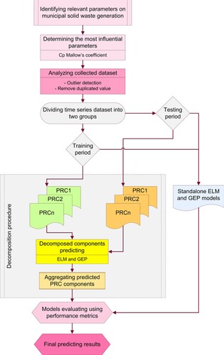
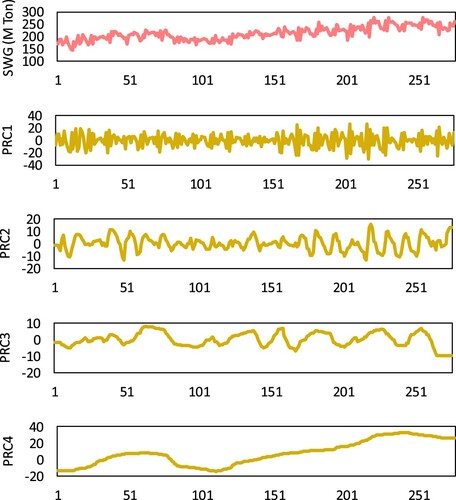
Figure 2. Decomposition results in PRCs and the residual of the monthly SWG.

The idea of decomposing and aggregating input data and then integrated with two DDM techniques (ITD-GEP and ITD-OPELM) formulates an accurate estimation of SWG with ten input values in Tehran megacity. The decomposed input data can simplify the data structure, and aggregating help the modelers to generate an appropriate formula. Finally, to define the best model, all generated models are evaluated with statistical performance metrics.

As stated above, ITD method is used to decompose input data signals into several PRCs to extract the main components. Searching the pattern of input data series and changing these patterns from high dimensions to lower dimensions is essential. Figure 2 demonstrates the initial SWG data in pink color. ITD method decomposes SWG data into four permanent PRCs and the residual lines, which are shown in yellow color (with the x-axis of the month). From Figure 2, it is evident that the sum of all PRCs results in the input signal.

3. Case study and data collection

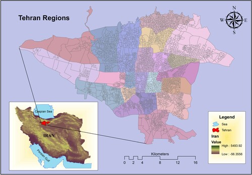
Tehran, the capital city of Iran, is located in the slope of central Alborz mountain between the 35° 42’ 55.0728” N and 51° 24’ 15.6348” E. The area of Tehran is over 700 km² with approximately 12.5 million population, which is the largest city of Iran. Moreover, the elevation of Tehran varies from 1800 m in the north, 1200 m in central, and 1050 m in southern parts. Tehran climate is categorized as semi-arid with an annual rainfall of 245–316 mm. The temperature of Tehran varies from a minimum of 18°C to a maximum of 38.7°C annually. TWMO has the duty of collecting waste, measuring its weight at landfill sites and reporting the data. A vast amount of waste (around 8000 Tons/day) is generated daily as a result of the massive population, according to TWMO. A significant proportion (70%) of waste belongs to organic and biodegradable waste wastes, which are almost categorized as wet waste. Figure 3 shows the map of the study area with input data for SWG modeling.

Figure 3. The study area (22 regions of Tehran) along with input waste generation data.

As mentioned above, there are lots of factors related to waste. Therefore, in this study, the parameters such as a month, rainfall, maximum temperature, average temperature, population, household size, educated man, educated women, GDP, and income, are selected from the period of 1991 to 2013 as input variables considering MSW as output in SWG modeling.

Some studies found that an increase in income can change the consumption patterns of households, resulting in changed composition and quantities of waste (Trang et al., 2017; Abbasi & El Hanandeh, 2016). According to Silva et al. (2020), socio-economic factors such as income, education level and GDP also contribute significantly to variations in SWG. Climate change is one of the influential factors that is already happening due to human activities. It is founded that the world may experience changes in seasonal precipitation, higher temperatures, and more extreme rainfall events. In future, these changes can be effective on the range of economic, social, and environmental processes straightforwardly. Accordingly, waste generation activities are evolving due to economic, social, and environmental change (Bebb & Kersey, 2003).

The whole input data include 22 years of monthly data (274 months), 75% of which (207 months) are defined as training, and the remaining 25% (69 months) are selected as testing data. The statistical characteristics are shown in Table 1 for the training and testing periods.

Table 1. Statistical parameters of input and output variables.

Variables	Mean	Variance	Standard deviation	Min	Max	Skewness	Kurtosis
Training stage
Tave (°C)	18.137	90.33575	9.504512	1.1	32.5	−0.066	−1.391
Tmax (°C)	28.610	86.00275	9.273767	9.4	42.6	−0.241	−1.252
Rain (mm)	21.022	686.5978	26.20301	0	141.7	1.874	4.615
GDP (Rial)	38299122	1.01E+15	31744393	3866774	1.22E+08	0.812	−0.385
POP (Person)	7069734	1.99E+11	446260.4	6475527	8015894	0.728	−0.632
EM (Person)	3799458	2.73E+11	522176.5	3314022	5047863	1.260	0.156
EW (Person)	3627054	2.6E+11	509817.1	3161505	4825337	1.198	−0.020
HS	1969210	1.93E+11	439227.5	1468427	2920416	0.901	−0.553
Income (Rial)	27052.08	5.54E+08	23540.52	2840.826	88219.39	0.927	−0.231
Waste (MTon)	202.950	392.359	19.808	146.047	258.225	−0.047	−0.083
Testing stage
Tave (°C)	18.325	91.282	9.554	3.7	32.4	−0.043	−1.500
Tmax (°C)	28.829	88.340	9.399	13.4	42.6	−0.154	−1.451
Rain (mm)	17.899	419.798	20.489	0	105.2	1.693	4.007
GDP (Rial)	1.58E+08	5.35E+14	23124151	1.22E+08	1.87E+08	−0.244	−1.445
POP (Person)	8068212	1.67E+10	129184	7820192	8300546	−0.073	−0.879
EM (Person)	4221856	4.47E+11	668394.3	4079492	8184822	5.617	31.937
EW (Person)	4157739	4.66E+11	682835.5	3906769	8184822	5.529	31.250
HS	2620437	9.03E+11	950442.7	2258688	8184822	5.514	31.111
Income (Rial)	122096.6	1.6E+09	40056	88219.39	204549.2	1.341	0.362
Waste (MTon)	246.084	266.239	16.317	199.228	276.856	−0.451	−0.043

4. Model assessment criteria

The reliability of the proposed models is evaluated using several statistical criteria including coefficient of determination (R²), root mean square error (RMSE), percent mean absolute relative error (PMARE), uncertainty at 95% (U95), Willmott’s index of agreement (WI), which are computed as follows: (16) $\begin{array}{rl}{R}^2& ={\left(\frac{\begin{array}{c}\sum _{i=1}^N\left(SW{G}_o-\overline{SW{G}_o}\right)\\ \left(SW{G}_m-\overline{SW{G}_m}\right)\end{array}}{\sqrt{\begin{array}{c}\sum _{i=1}^N{\left(SW{G}_o-\overline{SW{G}_o}\right)}^2\\ \sum _{i=1}^N{\left(SW{G}_m-\overline{SW{G}_m}\right)}^2\end{array}}}\right)}^2,\\ & \text{ ideal value}=1\end{array}$(16) (17) $\begin{array}{rl}RMSE& =\sqrt{\frac{1}{N}\sum _{i=1}^N{\left(SW{G}_m-SW{G}_o\right)}^2},\\ & \text{ ideal value}=0\end{array}$(17) (18) $\begin{array}{rl}PMARE& =\frac{100}{N}\sum _{i=1}^N(SW{G}_m-SW{G}_o{)}^2,\\ & \text{ideal value}=0\end{array}$(18) (19) $\begin{array}{rl}{U}_{95}& =1.96\sqrt{\left(STDE{V}^2+RMS{E}^2\right)}\\ & \text{ideal value}=0\end{array}$(19) (20) $\begin{array}{rl}WI& =1-\left[\frac{\sum _{i=1}^N{\left(SW{G}_0-SW{G}_m\right)}^2}{\begin{array}{c}\sum _{i=1}^N(|SW{G}_m-\overline{SW{G}_o}|\\ +|SW{G}_o-\overline{SW{G}_o}|{)}^2\end{array}}\right],\\ & \text{ideal value}=1\end{array}$(20) where, $SW{G}_o$ and $SW{G}_m\text{ denote }$ the observed and modeled values of SWG, respectively. Besides, $\overline{SW{G}_o}$ and $\overline{SW{G}_m}$ denote the average values of observed and modeled SWG data, respectively, and N is the number of the entire data.

5. Application results and discussion

After having decomposed input parameters of MSW time series data with ITD algorithm, CP coefficient is used to decrease the model complexity and unessential parameters are omitted. Afterward, two important DDMs, namely GEP and OPELM, are employed in MSW prediction. The advantage of considering these DDMs (GEP and OPELM) is that they consider operational parameters and are able to give a functional set of input variables as well as constant variables.

5.1. Determining optimum input variables

The best subset of input variables is selected by Mallow’s coefficient. Mallow’s CP is the best way to simplify the highest number of parameters (Fadaee et al., 2020). The results of the optimum input variables in SWG modeling are demonstrated in Table 2. This table provides R², CP, and standard deviation of all input variables. Ten subsets and models are structured, considering input variables for SWG forecasting. It can be seen that some parameters, including M, T_ave, GDP, HS, and income in model number 5, with the lowest CP value, are the most critical parameters. While considering R² values, models 5–10 are close to one another. The reported values of R², CP, and Stdev for the selected subset are 71.4, 9.9, and 146.27, respectively.

Table 2. Values of Mallows’ CP results from best subsets regression analysis.

				Variables
Model No.	R^2	CP	Stdev.	M	Tmax	Tave	Rain	GDP	POP	EM	EW	HS	Income
1	62.5	76.1	163.59					X
2	66.5	29.8	155.75		X			X
3	67.8	14.6	151.69			X		X					X
4	68.7	12.7	149.68	X	X			X					X
5	71.4	9.9	146.27	X		X		X				X	X
6	71.4	11.4	146.42	X		X		X	X		X		X
7	71.4	11.4	146.23	X		X	X	X	X			X	X
8	71.5	11.8	145.51	X		X	X	X	X		X	X	X
9	71.5	12.5	145.37	X	X	X	X	X	X		X	X	X
10	71.5	13.1	145.25	X	X	X	X	X	X	X	X	X	X

5.2. Stand-alone model configuration

The primary aim of this section is to define the selected model’s parameters along with their initializations (GEP and OPELM models). Thus, the following subsections discuss each model’s parameters and scenarios.

5.2.1. Development of the GEP model

Table 3 demonstrates input parameters such as function set (+, −, ×, /, exp, power) used in this study with trial and error. The mutation and inversion rate are set as 0.138 and 0.546, respectively. Gene recombination and transportation rate are defined to have the same value as 0.277. The maximum tree depth in each node is selected as 6 and the number of chromosomes is 30 along with three genes.

Table 3. Setting parameters of GEP model for SWG prediction.

Parameters	Description of parameters	Setting of parameters
P1	Function set	+, −, ×, /, exp, power
P2	Mutation rate	0.138
P3	Inversion rate	0.546
P4	One point and two-point recombination rate respectively (%)	0.277
P5	Gene recombination rate	0.277
P6	Gene transportation rate	0.277
P7	Maximum tree depth	6
P8	Number of gene	3
P9	Number of chromosomes	30

The results of SWG modeling with stand-alone GEP are demonstrated in two ways, including the obtained formula along with the decision tree. Based on CP results, a group of parameters including HS, income, m, T_ave, GDP is selected to form the SWG equation by GEP programming. Figure 4 demonstrates the three subsets of the decision tree in SWG forecasting using the GEP model. Moreover, Table 4 provides SWG non-linear mathematical formula (ET_Total) using the optimally selected variables (from CP), which is generated by GEP method.

Figure 4. The decision tree of the GEP model.

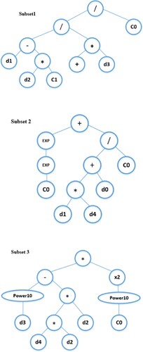
Table 4. Non-linear mathematical formula for SWG in each GEP subset.

Number of ET	Equation
Sub-ET1	$-0.8249\times \left[HS-\left(-5.1899\times \text{Income}\right)\right]/\left(-0.8249M+M^2\right)$
Sub-ET2	$178445072.9+\left[\left(HS\times T_{\text{avg}}\right)+GDP/2.944\right]$
Sub-ET3	$\left[{10}^M-(T_{\text{avg}}\times \text{Incom}{\text{e}}^2\right]/100000$
ETTotal	$\sum _{i=1}^{3}Sub-E{T}_i$

5.2.2. Development of OPELM model

The main aim of designing OPELM algorithm is for vigorous improvement of stand-alone OPELM models in estimating SWG. To achieve this, an elegant OPELM algorithm is utilized by conducting MATLAB code. As previously mentioned, OPELM model scenarios start with the first step of input data training (considering the featured vectors). The second step is on the weight of the input layer for the hidden layer. The hidden matrix is computed in the third step. Next, the inverse of the hidden matrix is computed. Finally, the weight of the hidden layer is designed.

5.3. Comparison of the proposed models for SWG prediction

Tables 5 and 6 provide the performance metrics of four models in SWG forecasting, including GEP, OPELM, ITD-GEP, ITD-OPELM, and MC-based AI models in training and testing stages. For the training phase, the results indicate that by considering the squared R, MC-ITD-GEP model with 0.836 has the highest value, followed by ITD-GEP with 0.821, and then MC-ITD-OPELM and MC-GEP with the values of 0.813 and 0.782, respectively. Based on the root mean square error, MC-ITD-GEP has the lowest value (12.057 M Ton). U95 shows that with the 95% uncertainty confidence, MC-based ITD-GEP has the lowest uncertainty, which indicates that this model has the best performance among other models in SWG forecasting. By considering WI index as shown in Table 5, ITD-GEP with the help of Monte-Carlo resampling technique indicates a satisfactory result in SWG forecasting.

Table 5. The results of the evaluation criteria of the proposed methods in the training stage.

Performance metrics – Training
	R^2	RMSE (M Ton)	PMARE (M Ton)	U95	WI
GEP	0.777	12.621	4.645	56.912	0.923
OPELM	0.727	13.627	4.878	57.796	0.916
MC-GEP	0.782	12.254	4.519	56.758	0.928
MC-OPELM	0.763	12.852	4.798	57.058	0.921
ITD-GEP	0.821	12.279	4.310	56.624	0.942
ITD-OPELM	0.780	12.294	4.382	56.637	0.933
MC-ITD-GEP	0.836	12.057	4.128	55.951	0.957
MC-ITD-OPELM	0.813	12.158	4.221	56.384	0.942

Table 6. The results of the evaluation criteria of the proposed methods in the testing stage.

Performance metrics – Testing
	R^2	RMSE (M Ton)	PMARE (M Ton)	U95	WI
GEP	0.610	13.881	5.845	45.804	0.775
OPELM	0.456	18.183	7.663	51.263	0.651
MC-GEP	0.685	12.368	4.928	42.681	0.795
MC-OPELM	0.612	14.254	6.621	47.627	0.789
ITD-GEP	0.735	12.194	5.195	43.920	0.868
ITD-OPELM	0.516	16.014	6.910	48.404	0.701
MC-ITD-GEP	0.782	11.557	4.621	41.624	0.877
MC-ITD-OPELM	0.62	13.025	5.257	44.339	0.792

The results in the testing stage (Table 6) also demonstrate satisfactory results on the applicability of MC resampling with ensemble ITD-GEP and ITD-OPELM models. By considering R² coefficient, MC-ITD-GEP has a higher value than the ITD-OPELM model. In other words, MC-ITD-GEP has 4.7% and 17.2% increases in accuracy in comparison to stand-alone GEP and ITD-GEP models. Considering RMSE, the error of ITD-GEP using MC technique decreases 1.22 units, while MC-ITD-OPELM error decreases 2.4 units in comparison to their stand-alone models. PMARE metric also demonstrates that MC-ITD-GEP method has the lowest error among other ensemble and stand-alone methods. The uncertainty in 95% of confidence level has the highest value for OPELM model in the testing stage. Finally, WI metric demonstrates that MC-ITD-GEP outperforms all other models.

The scatter plot outcomes of the selected models, including stand-alone GEP and OPELM, along with the coupled version of them (ITD-GEP and ITD-OPELM), are plotted in training and testing stages, which are illustrated in blue and red color, respectively (Figures 5 and 6).

Figure 5. The scatter plot of the proposed method in the Training stage.

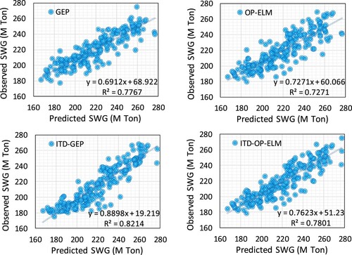
Figure 6. The scatter plot of the proposed method in the Testing stage.

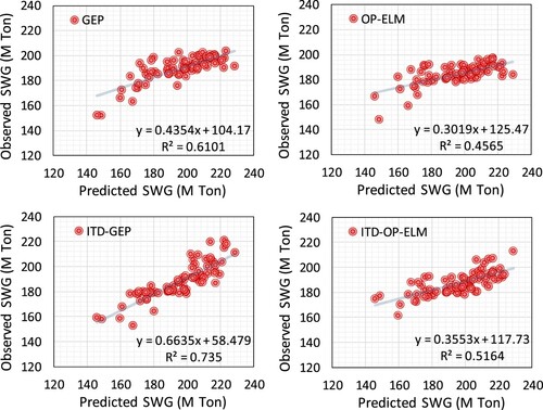
Figure 5 demonstrates the observed and predicted SWG (M Ton) in the training phase for stand-alone models (GEP, OPELM) and ITD integrated models (ITD-GEP and ITD-OPELM). As shown on the above left, the equation of y = 0.6912x + 69.922 demonstrates the relationship between two modeled and observed data sets, and the squared R has a satisfactory value (0.7767), which shows a proper fit between the observed and predicted SWG data. Considering R², OPELM method is followed by stand-alone GEP with a value of 0.7271. However, in the next step, by integrating novel signal processing ITD method with stand-alone models, the squared R values increase to 0.8214 for ITD-GEP and 0.7801 for ITD OPELM, respectively. Comparing the two ITD-hybrid models, ITD-GEP model with the equation of y = 0.8898x + 19.219 representing the observed and predicted values in SWG forecasting has more similarity than that of ITD-OPELM method. Thus, the best-performed method in training stage is ITD-GEP.

Figure 6 provides the information mentioned above for the testing stage, and stand-alone GEP and OPELM models are compared with their ITD-hybrid models utilizing the equation between predicted and observed SWG data. In comparison to the training information, the squared R values are smaller. Nevertheless, again in comparing stand-alone models, GEP outperforms the OPELM in SWG forecasting while in comparing the decomposed ITD-GEP and ITD-OPELM models, ITD-GEP model with the equation of y = 0.6635x + 58.479 and R² = 0.735 has the highest value and this model is selected as the best and accurate model in Tehran city SWG forecasting.

5.4. Further analysis and discussion

A clear understanding of waste generation is one of the essential issues in environmental studies like waste collection and waste treatment in cities, especially megacities in developing counties. Temperature, growing population, GDP, income, household size, number of educated people, etc. are critical parameters in controlling the generation of waste. Having information and historical data of each abovementioned parameter can aid policymakers to manage and make better decision. According to Pan et al. (2019), GDP and population parameters are essential variables in SWG in mega and super megacities, respectively. This study presents a case study on predicting the SWG formula in Tehran megacity in Iran. The best input values are selected using CP coefficient, including M, T_max, T_ave, Rain, GDP, POP, EM, EW, HS, and income. In this study, the applicability of stand-alone models (GEP and OPELM) are evaluated, and results of stand-alone models are combined with ITD-decomposed SWG input values. The results indicate that hybrid ITD-based models (ITD-GEP and ITD-OPELM) have the greatest similarity with the observed SWG data. Figure 7 depicts the time series of predicted and observed values of SWG (M Ton) on a monthly scale. The above plots provide error prediction charts for GEP (in red color), OPELM (in green color), ITD-GEP (in yellow color), and ITD-OPELM (in blue color). As shown in this figure, the error values are fluctuating between −22 and 40 in stand-alone GEP, −22 to 42 in stand-alone GEP and, for ITD based hybrid models, −15 to 30 for ITD-GEP and −30 to 30 for ITD-OPELM. The smallest fluctuation in error shows the best-performed model among all models.

Figure 7. The error prediction plots for SWG predicted time series of the proposed models with historical SWG series.

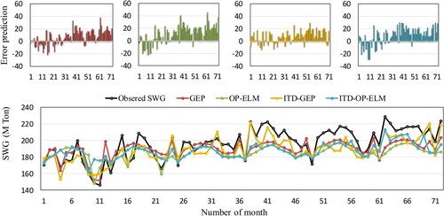
At last, by drawing all predicted SWG time series and comparison among all models, ITD based hybrid models outperform the two stand-alone models, and they improve the accuracy shortcomings of stand-alone GEP and OPELM models. Overall, ITD-GEP is nominated as the best-performed model in SWG forecasting.

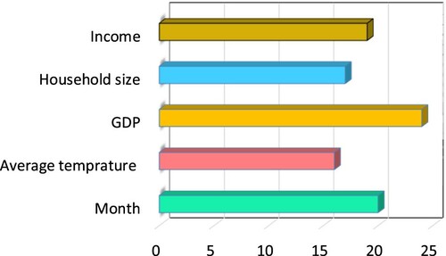
Another analysis that can be addressed in this study is the sensitivity analysis (SA) of variables, which indicates the effect of different values of predictors on target. For each predictor, SA% is as follows [53]: (21) $\begin{array}{rl}{L}_i& =t_{max}\left(x_i\right)-t_{min}\left(x_i\right)\end{array}$(21) (22) $\begin{array}{rl}S{A}_i& =\frac{L_i}{\sum _{j=1}^M{L}_i}\times 100\end{array}$(22) where t_max and t_min = maximum and minimum of the estimated target over the ith input domain, where other predictor values are equal to their average values. Results of variable importance in modeling municipal SWG are indicated in Figure 8 based on GEP model (the best stand-alone model). This figure indicates that the most effective variable in monthly SWG is GDP.

Figure 8. Result of the importance input variables on SWG using SA.

Overall, the performances of noise detection decomposition models (ITD-based) based on 22 years of SWG data are evaluated, and the results reveal that hybrid ITD-GEP and ITD-OPELM outperform their stand-alone models.

6. Conclusion

Since MSWG is an essential issue in the era of increasing population rate, it deserves to be simulated by DDMs to have better management. Many factors have significant influences on SWG, such as a month, Rain, Tmax, Tave, POP, HS, EM, EW, GDP, and income. Considering all parameters and factors as input parameters for designing an appropriate model takes much time and effort. In this regard, CP is utilized as FS technique to determine the optimum input parameters for SWG forecasting. After having defined the best inputs, two stand-alone DDMs, namely GEP and OPELM, are used in this study. As the first step, this study proposes a comprehensive and promising formula in order to predict monthly municipal SWG using less number of predictors and more influential ones. In addition, since the waste data are complex, non-stationary, and non-linear, ITD signal decomposing method is utilized to extract SWG input data features into straightforward and linear baseline signals of predominant PRCs. The critical aspect of ITD based methods is that they generate piecewise linear operators, which render the models easy and faster computation. Decomposing the input data into several PRCs, then modeling with DDMs and aggregating them again in order to report the output value is the other important objective of this study. Then, Monte-Carlo resampling technique is used to handle imbalanced datasets. Several performance metrics, particularly R² and WI, and visual plots, demonstrate that by decomposing the nonstationary and nonlinear SWG into relatively stationary signals and appropriately overcoming the noise terms hidden inside the original SWG, prediction quantities can be improved significantly. Based on the sensitivity analysis, GDP is found as the most important variable on monthly SWG at Tehran, while the average temperature is less important than the rest. To sum up, in the present study, ensemble AI models is proposed, namely MC-ITD-GEP and MC-ITD-OPELM, in which MC-ITD-GEP model outperforms all other models for SWG prediction. Since waste management is a significant issue, future works should be undertaken on SWG prediction using brand-new methods considering other relevant parameters as input.

Acknowledgements

The open access funding by the publication fund of the TU Dresden.

Disclosure statement

No potential conflict of interest was reported by the author(s).

Additional information

Funding

This work is supported by Fund for Reserve Academic Leader 2020–2022 granted by Capital University of Economics and Business and Special Fund for Fundamental Scientific Research of the Beijing Colleges in CUEB granted by Capital University of Economics and Business.

References

- Abbasi, M., & El Hanandeh, A. (2016). Forecasting municipal solid waste generation using artificial intelligence modelling approaches. Waste Management, 56, 13–22. https://doi.org/https://doi.org/10.1016/j.wasman.2016.05.018
- Abbasi, M., Rastgoo, M. N., & Nakisa, B. (2019). Monthly and seasonal modeling of municipal waste generation using radial basis function neural network. Environmental Progress and Sustainable Energy, 38(3), e13033. https://doi.org/https://doi.org/10.1002/ep.13033
- Abdulredha, M., Abdulridha, A., Shubbar, A. A., Alkhaddar, R., Kot, P., & Jordan, D. (2020). Estimating municipal solid waste generation from service processions during the Ashura religious event. IOP Conference Series: Materials Science and Engineering, 671(1), 012075. https://doi.org/https://doi.org/10.1088/1757-899X/671/1/012075
- Ali Abdoli, M., Falah Nezhad, M., Salehi Sede, R., & Behboudian, S. (2012). Longterm forecasting of solid waste generation by the artificial neural networks. Environmental Progress & Sustainable Energy, 31(4), 628–636. https://doi.org/https://doi.org/10.1002/ep.10591
- Araiza-Aguilar, J. A., Rojas-Valencia, M. N., & Aguilar-Vera, R. A. (2020). Forecast generation model of municipal solid waste using multiple linear regression. Global Journal of Environmental Science and Management, 6(1), 1–14. https://doi.org/https://doi.org/10.22034/gjesm.2020.01.01
- Arena, U., Mastellone, M. L., & Perugini, F. (2003). The environmental performance of alternative solid waste management options: A life cycle assessment study. Chemical Engineering Journal, 96(1–3), 207–222. https://doi.org/https://doi.org/10.1016/j.cej.2003.08.019
- Ashrafian, A., Shokri, F., Taheri Amiri, M. J., Yaseen, Z. M., & Rezaie-Balf, M. (2020). Compressive strength of foamed cellular lightweight concrete simulation: New development of hybrid artificial intelligence model. Construction and Building Materials, 230, 117048. https://doi.org/https://doi.org/10.1016/j.conbuildmat.2019.117048
- Azarmi, S. L., Oladipo, A. A., Vaziri, R., & Alipour, H. (2018). Comparative modelling and artificial neural network inspired prediction of waste generation rates of hospitality industry: The case of North Cyprus. Sustainability (Switzerland), 10(9), 2965. https://doi.org/https://doi.org/10.3390/su10092965
- Bebb, J., & Kersey, J. (2003). Potential impacts of climate change on waste management. Environment Agency. https://assets.publishing.service.gov.uk
- Benítez, S. O., Lozano-Olvera, G., Morelos, R. A., & Vega, C. A. (2008). Mathematical modeling to predict residential solid waste generation. Waste Management, 28(Suppl. 1), 7–13. https://doi.org/https://doi.org/10.1016/j.wasman.2008.03.020
- Bokde, N. D., Yaseen, Z. M., & Andersen, G. B. (2020). ForecastTB – An R package as a test-bench for time series forecasting – Application of wind speed and solar radiation modeling. Energies, 13(10), 2578. https://doi.org/https://doi.org/10.3390/en13102578
- Cevik, S., Cakmak, R., & Altas, I. H. (2017). A day ahead hourly solar radiation forecasting by artificial neural networks: A case study for Trabzon province. 2017 International Artificial Intelligence and Data Processing Symposium (IDAP), Malatya, Turkey. https://doi.org/https://doi.org/10.1109/idap.2017.8090223
- Chhay, L., Reyad, M. A. H., Suy, R., Islam, M. R., & Mian, M. M. (2018). Municipal solid waste generation in China: Influencing factor analysis and multi-model forecasting. Journal of Material Cycles and Waste Management, 20(3), 1761–1770. https://doi.org/https://doi.org/10.1007/s10163-018-0743-4
- Duan, N., Li, D., Wang, P., Ma, W., Wenga, T., Zhong, L., & Chen, G. (2020). Comparative study of municipal solid waste disposal in three Chinese representative cities. Journal of Cleaner Production, 254, 120134. https://doi.org/https://doi.org/10.1016/j.jclepro.2020.120134
- El-Fadel, M., Findikakis, A. N., & Leckie, J. O. (1997). Environmental impacts of solid waste landfilling. Journal of Environmental Management, 50(1), 1–25. https://doi.org/https://doi.org/10.1006/jema.1995.0131
- Fadaee, M., Mahdavi-Meymand, A., & Zounemat-Kermani, M. (2020). Seasonal short-term prediction of dissolved oxygen in rivers via nature-inspired algorithms. CLEAN – Soil, Air, Water, 48(2), 1900300. https://doi.org/https://doi.org/10.1002/clen.201900300
- Feng, Y., Cui, N., Zhao, L., Hu, X., & Gong, D. (2016). Comparison of ELM, GANN, WNN and empirical models for estimating reference evapotranspiration in humid region of Southwest China. Journal of Hydrology, 536, 376–383. https://doi.org/https://doi.org/10.1016/j.jhydrol.2016.02.053
- Fernandez Martinez, R., Okariz, A., Ibarretxe, J., Iturrondobeitia, M., & Guraya, T. (2014). Use of decision tree models based on evolutionary algorithms for the morphological classification of reinforcing nano-particle aggregates. Computational Materials Science, 92, 102–113. https://doi.org/https://doi.org/10.1016/j.commatsci.2014.05.038
- Ferreira, C. (2001). Gene expression programming in problem solving. Soft Computing in Industry – Recent Applications, 1996(7), 641–660. https://doi.org/https://doi.org/10.1007/978-1-4471-0123-9_54
- Fox, J. L. (2002, May). Comparison of a Monte Carlo calculation of the escape rate of C from Mars to that obtained using the exobase approximation. AGU Spring Meeting Abstracts (Vol. 2002, pp. SA41A-23).
- Frei, M. G., & Osorio, I. (2007). Intrinsic time-scale decomposition: Time–frequency–energy analysis and real-time filtering of non-stationary signals. Proceedings of the Royal Society A: Mathematical, Physical and Engineering Sciences, 463(2078), 321–342. https://doi.org/https://doi.org/10.1098/rspa.2006.1761
- Ghaemi, A., Rezaie-Balf, M., Adamowski, J., Kisi, O., & Quilty, J. (2019). On the applicability of maximum overlap discrete wavelet transform integrated with MARS and M5 model tree for monthly pan evaporation prediction. Agricultural and Forest Meteorology, 278, 107647. https://doi.org/https://doi.org/10.1016/j.agrformet.2019.107647
- Heddam, S., & Kisi, O. (2017). Extreme learning machines: A new approach for modeling dissolved oxygen (DO) concentration with and without water quality variables as predictors. Environmental Science and Pollution Research, 11(8), 1–23. https://doi.org/https://doi.org/10.1007/s11356-017-9283-z
- Hoque, M., & Rahman, M. T. U. (2020). Landfill area estimation based on solid waste collection prediction using ANN model and final waste disposal options. Journal of Cleaner Production, 256, 120387. https://doi.org/https://doi.org/10.1016/j.jclepro.2020.120387
- Huang, G.-B., & Chen, L. (2006). Universial approximation using incremental constructive feedforward neural networks with random hidden nodes. Transactions on Neural Networks, 17(4), 879–892. https://doi.org/https://doi.org/10.1109/TNN.2006.875977
- Iqbal, M. F., Feng, Q., Azim, I., Zhu, X., Yang, J., Javed, M. F., & Rauf, M. (2020). Prediction of mechanical properties of Green concrete incorporating waste foundry sand based on gene expression programming. Journal of Hazardous Materials, 384, 121322. https://doi.org/https://doi.org/10.1016/j.jhazmat.2019.121322
- Kannangara, M., Dua, R., Ahmadi, L., & Bensebaa, F. (2018). Modeling and prediction of regional municipal solid waste generation and diversion in Canada using machine learning approaches. Waste Management, 74, 3–15. https://doi.org/https://doi.org/10.1016/j.wasman.2017.11.057
- Kisi, O., & Kilic, Y. (2015). An investigation on generalization ability of artificial neural networks and M5 model tree in modeling reference evapotranspiration. Theoretical and Applied Climatology, 6(10). https://doi.org/https://doi.org/10.1007/s00704-015-1582-z
- Kisi, O., & Parmar, K. S. (2016). Application of least square support vector machine and multivariate adaptive regression spline models in long term prediction of river water pollution. Journal of Hydrology, 534, 104–112. https://doi.org/https://doi.org/10.1016/j.jhydrol.2015.12.014
- Kisi, O., Parmar, K. S., Soni, K., & Demir, V. (2017). Modeling of air pollutants using least square support vector regression, multivariate adaptive regression spline, and M5 model tree models. Air Quality, Atmosphere & Health, 10, 873–883. https://doi.org/https://doi.org/10.1007/s11869-017-0477-9
- Kisi, O., Sanikhani, H., & Cobaner, M. (2017). Soil temperature modeling at different depths using neuro-fuzzy, neural network, and genetic programming techniques. Theoretical and Applied Climatology, 129, 833–848. https://doi.org/https://doi.org/10.1007/s00704-016-1810-1
- Koza, J. R. (2007). What is genetic programming (GP). How Genetic Programming Works.
- Kumar, A., Samadder, S. R., Kumar, N., & Singh, C. (2018). Estimation of the generation rate of different types of plastic wastes and possible revenue recovery from informal recycling. Waste Management, 79, 781–790. https://doi.org/https://doi.org/10.1016/j.wasman.2018.08.045
- Liu, J., Li, Q., Gu, W., & Wang, C. (2019). The impact of consumption patterns on the generation of municipal solid waste in China: Evidences from provincial data. International Journal of Environmental Research and Public Health, 16(10), 1717. https://doi.org/https://doi.org/10.3390/ijerph16101717
- Miche, Y., Sorjamaa, A., Bas, P., Simula, O., Jutten, C., & Lendasse, A. (2010). OP-OPELM: Optimally pruned extreme learning machine. IEEE Transactions on Neural Networks, 21(1), 158–162. https://doi.org/https://doi.org/10.1109/TNN.2009.2036259
- Modaresi, F., Araghinejad, S., & Ebrahimi, K. (2018). A comparative assessment of artificial neural network, generalized regression neural network, least-square support vector regression, and K-nearest neighbor regression for monthly streamflow forecasting in linear and nonlinear conditions. Water Resources Management, 32(1), 243–258. https://doi.org/https://doi.org/10.1007/s11269-017-1807-2
- Mohammadi, K., Shamshirband, S., Petković, D., Yee, P. L., & Mansor, Z. (2016). Using ANFIS for selection of more relevant parameters to predict dew point temperature. Applied Thermal Engineering, 96, 311–319. https://doi.org/https://doi.org/10.1016/J.APPLTHERMALENG.2015.11.081
- Mohammadpour, R., Shaharuddin, S., Chang, C. K., Zakaria, N. A., Ghani, A. A., & Chan, N. W. (2015). Prediction of water quality index in constructed wetlands using support vector machine. Environmental Science and Pollution Research, 22(8), 6208–6219. https://doi.org/https://doi.org/10.1007/s11356-014-3806-7
- Mosavi, A., Ozturk, P., Vajda, I., Torabi, M., Varkonyi-Koczy, A., & Istvan, V. (2019). A hybrid machine learning approach for daily prediction of solar radiation design optimization of electric machines view project quantification of margins and uncertainties view project a hybrid machine learning approach for daily prediction of solar radiation. https://doi.org/https://doi.org/10.1007/978-3-319-99834-3_35
- Mozhiarasi, V., Raghul, R., Speier, C. J., Benish Rose, P. M., Weichgrebe, D., & Srinivasan, S. V. (2020). Composition analysis of major organic fractions of municipal solid waste generated from Chennai. In Sustainable waste management: Policies and case studies (pp. 143–152). https://doi.org/https://doi.org/10.1007/978-981-13-7071-7_13
- Naghibi, S. A., Pourghasemi, H. R., & Abbaspour, K. (2018). A comparison between ten advanced and soft computing models for groundwater qanat potential assessment in Iran using R and GIS. Theoretical and Applied Climatology, 131(3–4), 967–984. https://doi.org/https://doi.org/10.1007/s00704-016-2022-4
- Najafzadeh, M., & Zeinolabedini, M. (2019). Prognostication of waste water treatment plant performance using efficient soft computing models: An environmental evaluation. Measurement: Journal of the International Measurement Confederation, 138, 690–701. https://doi.org/https://doi.org/10.1016/j.measurement.2019.02.014
- Nęcka, K., Szul, T., & Knaga, J. (2019). Identification and analysis of sets variables for of municipal waste management modelling. Geosciences, 9(11), 458. https://doi.org/https://doi.org/10.3390/geosciences9110458
- Olejnik, S., Mills, J., & KesOPELMan, H. (2000). Using Wherry’s adjusted R2 and Mallow’s CP for model selection from all possible regressions. Journal of Experimental Education, 68(4), 365–380. https://doi.org/https://doi.org/10.1080/00220970009600643
- Oliveira, V., Sousa, V., & Dias-Ferreira, C. (2019). Artificial neural network modelling of the amount of separately-collected household packaging waste. Journal of Cleaner Production, 210, 401–409. https://doi.org/https://doi.org/10.1016/j.jclepro.2018.11.063
- Pan, Z., Chan, W. P., Veksha, A., Giannis, A., Dou, X., Wang, H., Lisak, G., & Lim, T. T. (2019). Thermodynamic analyses of synthetic natural gas production via municipal solid waste gasification, high-temperature water electrolysis and methanation. Energy Conversion and Management, 202, 112160. https://doi.org/https://doi.org/10.1016/j.enconman.2019.112160
- Şahin, M. (2013). Comparison of modelling ANN and ELM to estimate solar radiation over Turkey using NOAA satellite data. International Journal of Remote Sensing, 34(21), 7508–7533. https://doi.org/https://doi.org/10.1080/01431161.2013.822597
- Samal, B., Mani, S., & Madguni, O. (2020). Open dumping of waste and its impact on our water resources and health – A case of New Delhi, India. https://doi.org/https://doi.org/10.1007/978-981-15-0990-2_10
- Sattar, A. A., Elhakeem, M., Rezaie-Balf, M., Gharabaghi, B., & Bonakdari, H. (2019). Artificial intelligence models for prediction of the aeration efficiency of the stepped weir. Flow Measurement and Instrumentation, 65, 78–89. https://doi.org/https://doi.org/10.1016/j.flowmeasinst.2018.11.017
- Shiri, J., Keshavarzi, A., Kisi, O., Karimi, S., & Iturraran-Viveros, U. (2017). Modeling soil bulk density through a complete data scanning procedure: Heuristic alternatives. Journal of Hydrology, 549, 592–602. https://doi.org/https://doi.org/10.1016/j.jhydrol.2017.04.035
- Shiri, J., Sadraddini, A. A., Nazemi, A. H., Kisi, O., Marti, P., Fard, A. F., & Landeras, G. (2013). Evaluation of different data management scenarios for estimating daily reference evapotranspiration. Hydrology Research, 44(6), 1058–1070. https://doi.org/https://doi.org/10.2166/nh.2013.154
- Silva, L. J., da Santos, V. B., dos, I. F. S., Mensah, J. H. R., Gonçalves, A. T. T., & Barros, R. M. (2020). Incineration of municipal solid waste in Brazil: An analysis of the economically viable energy potential. Renewable Energy, 149, 1386–1394. https://doi.org/https://doi.org/10.1016/j.renene.2019.10.134
- Soni, U., Roy, A., Verma, A., & Jain, V. (2019). Forecasting municipal solid waste generation using artificial intelligence models – A case study in India. SN Applied Sciences, 1(2), 162. https://doi.org/https://doi.org/10.1007/s42452-018-0157-x
- Tenodi, S., Krčmar, D., Agbaba, J., Zrnić, K., Radenović, M., Ubavin, D., & Dalmacija, B. (2020). Assessment of the environmental impact of sanitary and unsanitary parts of a municipal solid waste landfill. Journal of Environmental Management, 258, 110019. https://doi.org/https://doi.org/10.1016/j.jenvman.2019.110019
- Trang, P. T. T., Dong, H. Q., Toan, D. Q., Hanh, N. T. X., & Thu, N. T. (2017). The effects of socio-economic factors on household solid waste generation and composition: A case study in Thu Dau Mot, Vietnam. Energy Procedia, 107, 253–258. https://doi.org/https://doi.org/10.1016/j.egypro.2016.12.144
- Vu, H. L., Ng, K. T. W., & Bolingbroke, D. (2019). Time-lagged effects of weekly climatic and socio-economic factors on ANN municipal yard waste prediction models. Waste Management, 84, 129–140. https://doi.org/https://doi.org/10.1016/j.wasman.2018.11.038
- Wei, C.-C. (2017). Predictions of surface solar radiation on tilted solar panels using machine learning models: A case study of Tainan city, Taiwan. Energies, 10(10), 1660. https://doi.org/https://doi.org/10.3390/en10101660
- Wen, Z., Chen, C., Ai, N., Bai, W., Zhang, W., & Wang, Y. (2019). Environmental impact of carbon cross-media metabolism in waste management: A case study of municipal solid waste treatment systems in China. Science of the Total Environment, 674, 512–523. https://doi.org/https://doi.org/10.1016/j.scitotenv.2019.04.154
- Zamani Sabzi, H., King, J. P., & Abudu, S. (2017). Developing an intelligent expert system for streamflow prediction, integrated in a dynamic decision support system for managing multiple reservoirs: A case study. Expert Systems with Applications, 83, 145–163. https://doi.org/https://doi.org/10.1016/j.eswa.2017.04.039
- Zeng, J., Wang, G., Zhang, F., & Ye, J. (2012). The de-noising algorithm based on intrinsic time-scale decomposition. Advanced Materials Research, 422, 347–352. https://doi.org/https://doi.org/10.4028/www.scientific.net/AMR.422.347
- Zeng, W., Ismail, S. A., & Pappas, E. (2020). '. Artificial Intelligence Review, 53, 3231–3253. https://doi.org/https://doi.org/10.1007/s10462-019-09761-0
- Zeng, W., Li, M., Yuan, C., Wang, Q., Liu, F., & Wang, Y. (2020). Identification of epileptic seizures in EEG signals using time-scale decomposition (ITD), discrete wavelet transform (DWT), phase space reconstruction (PSR) and neural networks. Artificial Intelligence Review, 53, 3059–3088. https://doi.org/https://doi.org/10.1007/s10462-019-09755-y