Simulation based investigation of 2D soft-elastic reactors for better mixing performance

Abstract

Inspired by the animal upper digestive tract, a unique soft-elastic reactor (SER) has recently been researched whose mixing phenomena should be further investigated. Numerical simulation is an excellent method with which to explore the phenomena in SERs for a large number of conditions. It may also offer insights into the ways of effective mixing in this kind of reactor. The mixing processes in 2D SERs driven by bio-inspired wavelike boundary motions are systematically compared in this work. The influences of several key factors (i.e. the aspect ratios of rectangular SERs, the wavenumbers of moving walls, and the location and size of baffles) on the mixing performance are investigated. It has been found that mixing efficiency is better at an aspect ratio close to 1.0. The influence of wavenumber on mixing is not monotonic. Increasing the wavenumber speeds up mixing in parallel boundary type motion, while it slows it down in symmetrical-contraction boundary type motion. Mounting baffles on the left and right sides of the vessel wall (i.e. on the moving boundaries) promotes mixing. Lower porosity (≤ 0.4) of baffles benefits mixing. It has become clear that an efficient SER needs to be designed by considering not only its shape but also the wall moving mode. The work reported in this article has provided useful information on how it might be possible to improve SERs for industrial applications in future.

KEYWORDS:

• Soft-elastic reactor (SER)
• numerical simulation
• mixing performance
• wall moving mode
• baffles

1. Introduction

Biology is a rich source of innovative ideas that can be the inspiration to find successful alternatives for solving specific and challenging problems in the chemical industry (Chen, 2016; Coppens, 2012). Chemical engineering equipment and processes, designed and built by imitating biological systems (including physical, chemical and mechanical structures), can lead to superb performance (Chen, 2016). The digestive systems of people and animals can be thought of as a series of miniature chemical reactors in which various unit operations occur (Chen & Yoo, 2006). The muscle tissues of the digestive organs exhibit peristaltic movements (a series of wavelike muscle contractions), and there is no mixing device (e.g. static mixer or impeller) in the lumen to promote the mixing. From an engineering viewpoint, the digestive tract is composed of multiple soft chemical reactors (Chen, 2016). These chemical reactors are special since none of them has a conventional agitation devices inside. They can be classified as soft-elastic reactors, whose walls are not rigid and the mixing is initiated by wall movements (Liu, Xiao, et al., 2018). The digestive tract can effectively enhance the mixing, crushing and transport of chyme, which mainly attributes to the physiological structure and wall motion of the digestive system (Liu, Xiao, et al., 2018; Liu, Zou, et al., 2018). In recent years, biological reactors in the digestive tract have gained more and more attention (Ji et al., 2021; Li, Yu, et al., 2020; Li, Zhu, et al., 2020; Wu & Chen, 2020). Chen et al. carried out food digestion studies using ‘near real’ in vitro digestive systems. Those systems take into account the physical movements, digestion environment and realistic morphology of digestive organs. For example, the human stomach system was used to investigate the effects of gastric morphology (including the complex geometrical shape and internal wrinkles) on emptying behaviors (Chen et al., 2016). The soft tubular model reactor was used to mimic the small intestine, based on which Deng et al. (2016) concluded that the movement of the reactor wall can accelerate starch hydrolysis. The rat stomach model, fabricated with the aid of 3D-printing technology, was used to explore the effects of the injection pattern of the gastric juice and the contraction frequency on the digestibility of casein powder suspensions (Zhang et al., 2018). Extended from those efforts, a prototype soft-elastic reactor (SER) was constructed to offer one potential alternative to traditional mixing equipment with rigid walls and agitators (Liu, Xiao, et al., 2018; Liu, Zou, et al., 2018). It is a standard cylindrical-shaped container made from silicone, in which the mixing is induced by the wall deformation triggered by the periodic protrusion of a beater from one side of the vessel (Chen & Liu, 2015). It was found that the SER could effectively mix highly viscous fluids (Liu, Xiao, et al., 2018).

Although the preliminary numerical analyses of prototype SERs have shown the potential in mixing high viscosity fluid in an efficient way (Li et al., 2019; Zou et al., 2020), SERs can be improved still further (Delaplace et al., 2018, 2020). The SER in experiments has one fixed shape, and the wall motion is restricted to a one-sided simple movement. Thus mixing-intensification methods need to be explored further (Liu, Xiao, et al., 2018). Gaining in-depth understanding of the flow physics under different operations can help better designs of SERs to be found, thus providing more possibilities of industrial implementations. Computational Fluid Dynamics (CFD) has been applied extensively to investigate flow characteristics and is a recognized method for designing and optimizing devices in a broad range of conventional engineering applications (Gao et al., 2016; Liu et al., 2019; Mosavi et al., 2019; Shamshirband et al., 2020; Zhang et al., 2016). The method can also be applicable to the study of mixing in human digestive organs, such as the stomach and intestines, whose walls keep wriggling during digestion (Alokaily et al., 2019; Ferrua & Singh, 2010; Li et al., 2021; Li & Jin, 2021; Zha et al., 2021). This method is quite suited to analyse the mixing process in SERs for exploring various influencing factors, because carrying out in silico experiments can be cost effective, and comprehensive flow field data can be obtained. In previous works, numerical two-dimensional (2D) models of SERs were developed in ANSYS^® Fluent^®: Li et al. (2019) showed that larger amplitudes and higher frequencies of the moving wall can mix the viscous fluid efficiently by tracking the evolution of the flow fields; an annular SER showed that flow directions should be considered to promote convective mixing (Zou et al., 2020). In this work, an open source package (OpenFOAM^® v.1806) is used to explore potential factors further that may influence the mixing performance of SERs. Structured hexahedral meshes are used for all calculations, which can make the calculation more efficient and accurate. A rational design of a mixing container should take care of the geometric configuration and also how it mixes. From a geometrical perspective, a range of aspect ratios (the longer side $H$ to its shorter side $L$: $H/L$, $H$ and $L$ are indicated in Figure 2) are investigated in this wall-motion-driven and closed 2D mixer. Regarding the mixing method, two basic boundary moving modes are considered, inspired by the wavelike motion of the gastric system: Type 1 moves the left and right walls in parallel; Type 2 moves the walls in a wormlike symmetrical contraction manner, which imitates the segmentation motions of human small intestines. In addition, different wavenumbers of the moving boundaries based on the two motion types are taken into account. It is known that baffles (flow-directing or obstructing panels used in some industrial containers for mixing efficiency improvement) can promote mixing in an agitated vessel (Hashimoto et al., 2011), but whether baffles can influence mixing behaviors in such a soft-elastic system as well as how to configure baffle size and locations for better mixing performance are still open questions. This work implements baffles by a porous media modeling approach, the method was also adopted by Blanco-Aguilera et al. (2020) to account for the effects of baffles in an anaerobic–anoxic reactor.

In short, the objective of our study is to explore potential factors that could affect the mixing performance of SERs with gastrointestinal motility inspired wall motions. The flow characteristics in SERs are carefully analysed with CFD simulations. By implementing baffles and changing the aspect ratios as well as wall-movement parameters, various factors influencing the mixing are investigated. Many of them (e.g. complex wall-motions) are not possible with the current experimental setup. This work can give insights for future design and implementation of highly effective SERs in real industrial applications.

2. Model design and numerical methods

Movements of the left and right walls (a schematic description in Figure 1) are determined by prescribed mathematical formulas that give the position of the mesh points as a function of time, see Equations (1)–(4). These wall movements do not change the volume (or the area in 2D) of SERs, hence the total mass of the fluid is conserved. Moreover, based upon results of the present authors' previous experimental studies of the mixing behavior within an SER induced by a simple one-sided wall deformation (Chen & Liu, 2015; Liu, Xiao, et al., 2018; Liu, Zou, et al., 2018), it is assumed that these complex wall movements of the reactor can as well be realized by an experimental setup in future. The reactor is simplified as a closed 2D vessel without free surfaces: (1) $\text{Type 1 left}:x=ϵL\text{sin}\left(N\frac{2\pi y}{H}\right)\text{sin}\left(\frac{2\pi }{T}t\right)$(1) (2) $\text{Type 1 right}:x=ϵL\text{sin}\left(N\frac{2\pi y}{H}\right)\text{sin}\left(\frac{2\pi }{T}t\right)+L$(2) (3) $\text{Type 2 left}:x=ϵL\text{sin}\left(N\frac{2\pi y}{H}\right)\text{sin}\left(\frac{2\pi }{T}t\right)$(3) (4) $\text{Type 2 right}:x=-ϵL\text{sin}\left(N\frac{2\pi y}{H}\right)\sin \left(\frac{2\pi }{T}t\right)+L$(4) where $ϵ$ is the normalized deformation amplitude, which is defined as the deformation amplitude divided by the SER's length. The mesh point positions are denoted by $x$ (mm) and $y$ (mm). As shown in Figure 2, $L$ (mm) and $H$ (mm) are the length and height of the computational domain, respectively, $L_t$ (mm) and $H_t$ (mm) are the length and height of the tracer domain initially, $L_t$ is one fifth of $L$, $H_t$ is one fifth of $H$ in all calculations. $L_b$ (mm) and $T_b$ (mm) are the length and thickness of the baffle. The moving boundary deforms in a sine shape, and $N$ is the wavenumber (or the repetency of one wavelength) of the moving boundary. $T$ (s) is the period of the moving wall and $t$ (s) is the physical time. The parametric settings used for the study are summarized in Table 1. In the simulation, a fluid with a kinematic viscosity of 1.0 × 10⁻⁶ m²/s is used as an illustration (tracer). The tracer has the same physical properties as the bulk fluid. The mass diffusion coefficient of the tracer is 2.299 × 10⁻⁹ m²/s (Nakashima, 2000).

Figure 1. Wall movement illustration within a period. $\text{①}$, $\text{②}$, $\text{③}$ and $\text{④}$ represent the first, second, third and fourth quarters of the motion cycle from its start, respectively.

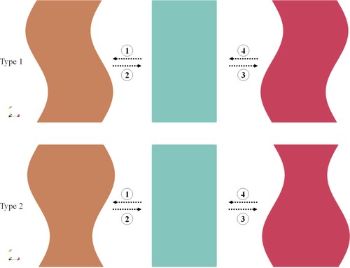
Figure 2. Schematic description of the numerical 2D model. The red rectangular area is located at the central part of the domain and represents the tracer initially distributed, the mass fraction of tracer is one inside and zero outside. The white stripes indicate baffles, which are modeled by porous media. Location 1 represents baffles implemented on bottom and top, Location 2 means baffles mounted on left and right.

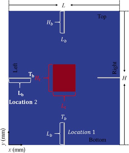
Table 1. Parameter values utilized in the simulation.

Parameters		Value	Notes
Mesh independence study	Grid numbers	12,000	50 × 60^a, 10 × 12^b, N = 1, baffles: no
		48,000
		192,000
		300,000
Effects of aspect ratios	Aspect ratio ($r_{hl}$^c)	1.20	50 × 60^a	10 × 12^b	N = 1, baffles: no
		1.875	40 × 75^a	8 × 15^b
		3.33	30 × 100^a	6 × 20^b
		4.80	25 × 120^a	5 × 24^b
		7.50	20 × 150^a	4 × 30^b
Effects of moving boundary wavenumbers	Wavenumber ($N$)	1	20 × 150^a, 4 × 30^b, baffles: no
		2
		3
Effects of baffles^d	Baffle length (mm)	5	50 × 60^a, 10 × 12^b, N = 1, baffles: 0.01 of porosity, Location 1 or Location 2
		10
		15
	Baffle porosity ($\varphi$)	0.01, 0.2, 0.4, 0.6, 0.8, 1.0, 0.8 on left and 0.01 on right	50 × 60^a, 10 × 12^b, N = 1, baffles: Location 2, 15 mm in length

^a $L\times H$ in millimeters; calculation domain area: 3000 mm². ^b$L_t\times H_t$ in millimeters; tracer domain area: 120 mm². ^c$r_{hl}=\left(H/L\right)$. ^dBaffle thickness: $T_b=0.25\text{mm}$. $ϵ=0.2$ and $T=6\text{s}$ are used in all simulations.

The fluid is considered to be incompressible and Newtonian. The flow in the SER is an isothermal, incompressible, single-phase flow. The continuity and momentum conservation equations are shown below (Ferziger et al., 2002; Schetz & Fuhs, 1999): (5) $\text{Continuity equation}:\frac{\mathrm{\partial }{u}_i}{\mathrm{\partial }{x}_i}=0$(5) (6) $\begin{array}{rl}& \text{Momentum equation}:\frac{\mathrm{\partial }{u}_i}{\mathrm{\partial }t}+\frac{\mathrm{\partial }\left(u_j{u}_i\right)}{\mathrm{\partial }{x}_j}\\ & =-\frac{\mathrm{\partial }p}{\mathrm{\partial }{x}_i}+\frac{\mathrm{\partial }{\tau }_{ij}}{\mathrm{\partial }{x}_j}-\mathrm{\Omega }\frac{\nu }{K}\left(u_i-u_{pi}\right)\end{array}$(6) where $u_{pi}$ (m/s) denotes the velocity of the moving mesh, $\nu$ (m²/s) is the kinematic viscosity of the fluid, $p$ (m²/s²) is the kinematic pressure, which is the static pressure divided by the density, $\mathrm{\Omega }$ is a dimensionless scalar, with $\mathrm{\Omega }=1$ at the baffle region and $\mathrm{\Omega }=0$ otherwise, the viscous stress tensor ${\tau }_{ij}$ (m²/s²) is calculated as (7) ${\tau }_{ij}=2\nu s_{ij}$(7) $s_{ij}=\frac{1}{2}\left(\frac{\mathrm{\partial }{u}_i}{\mathrm{\partial }{x}_j}+\frac{\mathrm{\partial }{u}_j}{\mathrm{\partial }{x}_i}\right)$ is the strain rate (s⁻¹). The permeability $K$ (m²) is defined using the Carman–Kozeny equation (Nield & Bejan, 2006): (8) $K=\frac{D_p^2{\varphi }^3}{180{\left(1-\varphi \right)}^2}$(8) which depends on the geometry of the medium rather than the fluid nature. $D_p$ (set to 1.6 mm) is the effective average diameter of solid grains in the porous media region (the region of the baffles). $\varphi$ is the porosity at the baffle region. It has to be mentioned that the body force term due to the porous baffles $\nu (u_i-u_{pi})/K$ is only accounted for in the baffle regions due to the introduced scalar $\mathrm{\Omega }$. In this system, the tracer is considered to be a dissolved solute. Hence, a species transport equation has to be solved to describe the tracer transport and to track the mixing process: (9) $\frac{\mathrm{\partial }C}{\mathrm{\partial }t}+\frac{\mathrm{\partial }\left(u_{i}C\right)}{\mathrm{\partial }{x}_i}=D_m\frac{{\mathrm{\partial }}^{2}C}{\mathrm{\partial }{x}_i^2}$(9)

Here, $C$ is the local mass fraction of the species, and $D_m$ (m²/s) is the mass diffusion coefficient for the species, which is relevant to the material properties. A finite volume method is employed for solving the above governing equations (5), (6) and (9). The solver used was developed based on the open source code package OpenFOAM^® v.1806. The solution scheme for time is the second-order implicit-backward method. The convection terms of equations (5), (6) and (9) are discretized with a second-order central difference scheme. The Poisson equation is used to determine the pressure at the new time step. The velocity is corrected by the Pressure-Implicit with Splitting of Operators (PISO) algorithm. To solve the continuity, momentum and species equations, suitable boundary conditions have to be imposed for $u_i$, $p$ and $C$, which are Neumann and Dirichlet boundary conditions when non-permeable walls are used (Ferziger et al., 2002). Zero gradient (Neumann type, $\left(\mathrm{\partial }\psi /\mathrm{\partial }t\right)=0$ and $\psi$ represents a general variable) boundary conditions are applied on the left, right, bottom and top boundaries for $p$ and $C$. No-slip boundary conditions (Dirichlet type) for $u_i$: a fixed value ($\psi ={\psi }_{\text{ref}}$, the reference value ${\psi }_{\text{ref}}=0$ is used for each velocity component) conditions are applied on the non-moving boundaries (e.g. the bottom and top); moving wall velocity conditions are applied on the moving boundaries (i.e. the left and right); the time dependent velocity is set by Equations (1)–(4).

3. Mixing performance quantification

The mixing performance is commonly evaluated by the mixing uniformity (or the mixing degree) (Delaplace et al., 2018, 2020; Hitimana et al., 2019; Xiao et al., 2018). In the laboratory, colorimetric methods are commonly used to characterize the mixing status (Cabaret et al., 2008; Liu, Xiao, et al., 2018). After the tracer is added to the system for further mixing, the concentration distribution of the tracer changes continuously as the mixing proceeds. In the current numerical model, a similar method is used to characterize the degree of mixing. As a result, at time $t$, the mixing level in the SER is calculated by (10) $\text{Mixing level}=\left(1-\frac{d_{\text{mix}}\left(t\right)}{d_{\text{mix}}\left(0\right)}\right)\times 100\mathrm{\%}$(10) $d_{\text{mix}}\left(t\right)$ is the averaged mixing difference at time $t$, which is defined as (11) $d_{\text{mix}}\left(t\right)=\underset{S}{\int }(C\left(t\right)-C_{\text{ideal}}{)}^2\text{d}S$(11) Here, $C\left(t\right)$ is the mass fraction in a certain cell at time $t$. $C_{\text{ideal}}$ is the mass fraction of an adequately mixed state (for instance, the ideal state or 100% homogeneity). $S$ (mm²) represents the area.

4. Results and discussion

4.1. Mesh independence study

Four meshes with different grid sizes are used to find a suitable mesh. The magnified views of the top-left corner are shown in Figure 3. For cases of the grid independence study, the SER without baffles, with $L\times H$ = 50 mm × 60 mm and $N=1$ is simulated. More computational information is given in Table 2.

Figure 3. Zoomed view of different meshes designed for the mesh independence study, the grids in the upper-left corner are shown. The computational domain has been divided into uniform and square cell elements, and their sizes are indicated respectively.

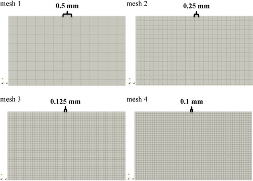
Table 2. Computational information for mesh independence study.

		Computational time (h)
Mesh ID^a	Processor number ($N_p$)^b	Type 1	Type 2
1	24	1.49	1.74
2	24	4.02	3.36
3	24	25.79	27.07
4	24	58.53	52.47

^a mesh 1: 100 × 120 × 1, mesh 2: 200 × 240 × 1, mesh 3: 400 × 480 ;× 1, mesh 4: 500 × 600 × 1. The grid number is written as $N_x\times N_y\times N_{\text{z}}$, where $N_x$, $N_y$ and $N_{\text{z}}$ are grid numbers in the x-, y- and z-directions, respectively. ^bThe calculations were carried out on one node of a cluster machine with CPU type 2 × E5–267.

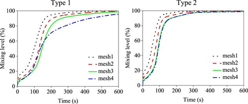
The velocity at half height of the reactor is monitored. In Figure 4, the velocities for different meshes are compared, and they show good agreement. As can be seen in Figure 5, the mixing level shows a similar trend for different mesh resolutions. In Type 1, the difference is more obvious between the various grid sizes, while in Type2, when the number of grids is increased from mesh 3 to mesh 4, the solution can be regarded as mesh independent. Thus, the subsequent simulations use mesh 3, which has 192,000 grid cells.

Figure 4. Velocity profiles at half height of SERs at $t$ = 600 s.

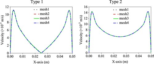
Figure 5. The mixing level evolution in the SER with four different meshes.

4.2. Effects of aspect ratios

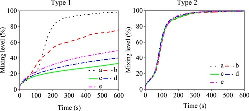
Here, the influence of the aspect ratio ($r_{hl}$) on the mixing is investigated. SER is operated with no baffles at $N=1$ for all aspect ratios considered. The chosen computational domains with different $L\times H$ are considered to ensure 2D SERs have the same area, and also to cover a relatively large range of aspect ratios, where the corresponding aspect ratios are 1.20, 1.875, 3.33, 4.80 and 7.50. It can be seen from Figure 6 that $r_{hl}$ has a great influence on Type 1 but not on Type 2. Overall, an $r_{hl}$ close to unity benefits the mixing more. The mixing level at 600 s (the end time of the mixing) decreases with the increase of $r_{hl}$ from (a) to (c), while it increases from (c) to (e) with increasing $r_{hl}$ in Type 1. In Type 2, $r_{hl}$ has no big influence on the mixing level and it has better performance than Type 1 at all values of $r_{hl}$.

Figure 6. The mixing level of different aspect ratios ($r_{hl}$). The $r_{hl}$ for (a), (b), (c), (d) and (e) are 1.20, 1.875, 3.33, 4.80 and 7.50, respectively.

To analyse differences better in the mixing performance of SERs with different values of $r_{hl}$, the effects of convective and diffusive mixing are considered in the mixing process. Convective mixing involves the bulk movement of the fluid. Diffusive mixing is caused by random motion of molecules. Generally, the mixing rate by diffusion is low compared with convection (Levy & Kalman, 2001). In the present model, owing to the small diffusion coefficient, convection is considered to be a main factor in the mixing; the rate of convective mass transfer is dependent on the extent of the fluid flow.

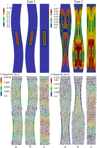
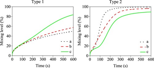
Here, we chose an $r_{hl}$ of 7.50 for further illustrations, because the mixing performance of two different motion types shows a huge difference. Figure 7 shows concentration distributions and corresponding flow fields for the two motion types at 200, 400 and 600 s, respectively. From the scalar field: The tracer does not spread obviously in Type 1 but spreads intensely in Type 2. The concentration distribution is left-right symmetrical in Type 2. From the velocity vector field: Type 1 moves fluid only in the horizontal direction, and there is no obvious transfer in the vertical direction (in general, the velocity vectors are horizontally aligned). It can also be seen that convective mixing is less important compared to Type 2, because the velocity magnitude is almost one order of magnitude smaller, especially in the central region. This is the case because Type 1 wall movements do not trigger any large vortical structures, which can be observed in the case with Type 2 wall movements. Type 2 has a stronger convection from the bottom to the top due to the contraction at the lower half. This symmetric contraction also causes a bilaterally symmetric velocity field; the two counter-rotating vortical structures are the skeleton of the flow. The reflectional symmetries of the velocity field are preserved in the flow, which will lead to inefficient mixing from one side to the other (mainly by means of diffusion). The reactor restores to its original shape at 600 s, and the velocity reaches its maximum, Type 2 has greater maximum velocity than Type 1. The central region of Type 1 tends to have its smallest velocity magnitude in the whole domain at different times, while Type 2 usually has its largest velocity magnitude in the central region. Flow field characteristics determine the tracer distribution and the mixing performance, which explains why Type 2 has better mixing performance in this operating condition. Through the analysis of direction, magnitude and distribution of flow velocity, the intensity of convection can be more accurately obtained. For SERs with the same size, the flow direction that is along the long side or has greater velocity can introduce more mass exchanges, and the high-velocity zone that distributes close to the tracer will also enhance tracer mixing.

Figure 7. Tracer concentration ($C$) and the corresponding flow field at different times for an $r_{hl}$ of 7.50: (a) t = 200 s; (b) t = 400 s; (c) t = 600 s.

4.3. Effects of moving boundary wavenumbers

For further investigating the influences of moving boundary wavenumbers on the mixing behavior, a greater aspect ratio of the computing domain has been chosen based on the research described above. The domain size used is $L\times H$ = 20 mm × 150 mm and the baffles are not taken into account. By using a higher SER, more wavenumbers can be implemented on the boundaries. As can be seen in Figure 8, (a) has one wavenumber (a crest and a trough) for each side, (b) has two wavenumbers and (c) has three wavenumbers. Figure 8 shows the tracer distribution at 400 s, which is at the state of maximum motion amplitude; all crests and troughs can be clearly seen at this time. The tracer distribution in Type 1 is rotationally symmetric, while that in Type 2 is left–right symmetric; this different distribution is determined by the corresponding boundary movements. From the range of the tracer distribution, Type 2 is larger than Type 1, and with increasing $N$ the tracer distribution zone in Type 1 is enlarging, while Type 2 shows the opposite trend.

Figure 8. The comparison of the tracer concentration ($C$) with different wavenumbers of moving boundaries at $t=400s$: (a) $N=1$; (b) $N=1$; (c) $N=3$.

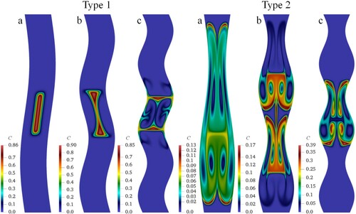
Figure 9 shows the change of mixing level over time. Type 2 has a higher mixing effect compared with that of Type 1 for the same wavenumbers. In Type 1, the increase in $N$ leads to an increase in the mixing level. In Type 2, fewer wavenumbers are beneficial to the mixing. This observation gives a clue to the fact that enhanced local convection may not improve global mixing efficiency. Greater numbers may increase the energy consumption and the operating complexity. For the special SER ($r_{hl}=7.50$) studied in this section, Type 2 motion mode with $N=1$ is the best option for improving global mixing efficiency. Type 2 with fewer motion waves introduces contractions on a large scale, which will significantly promote advections in the vertical direction. By increasing the number of waves, the fluid is trapped in a small region by more waves, see Figure 8 Type 2 (c), which prevents bulk flow in the vertical direction.

Figure 9. Mixing level as influenced by different wavenumbers of moving boundaries: (a) $N$ = 1; (b)$N$ = 1; (c) $N$ = 3.

4.4. Effects of baffles inside SER

The baffles are symmetrically implemented on the bottom and top (Location 1) or on the left and right (Location 2) in the SER, see Figure 2. The lengths of baffles ($L_b$) investigated in this study are 5, 10 and 15 mm, respectively, and the porosity ($\varphi$) of the modeled baffles is 0.01. The reactor is $L\times H$ = 50 mm × 60 mm in size and operates with $N=1$. The mixing effect of the reactor with baffles is compared to the cases without baffles. Figure 10 shows the variation of the mixing level over time for different lengths and locations of baffles. The baffles that are located at Location 2 can always enhance the mixing regardless of the length for both types. Mixing reaches a steady state within 100 s, and the mixing efficiency increases with increasing baffle length. Furthermore, the length increase from (a) to (b) has a stronger enhancement effect of the mixing efficiency than that from (b) to (c). For baffles at Location 1, the effect of the length variation influences the mixing efficiency in a different way. In Type 1, the mixing is significantly enhanced by the longest baffle; (a) mixes faster and also has a larger final mixing level compared to the unbaffled mixer; while for (b), it mixes faster in 0–190 s and slower afterwards, the final mixing level is also lower. In Type 2, the mixing efficiency of the baffled SER decreases, the mixing level curve of the shortest-baffle SER almost coincides with the unbaffled SER, the mixing quality is even inferior with longer baffles. To summarize, the location and length of baffles should be considered together with the SER motion types.

Figure 10. Mixing level changes over time as influenced by the length of baffles. The baffle lengths are 5, 10, 15 and 0 mm for (a), (b), (c) and (d), respectively.

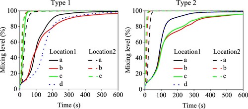
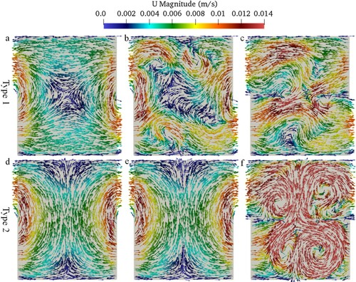
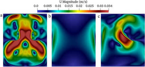
Figure 11 shows the flow field at 600 s, the arrow heads point out the flow direction and their color indicates the velocity magnitude. The presence of baffles produces new flow directions and a more disordered flow field. The flow speed is thus increased and the high velocity region is also enlarged. However, it's worth noting that no such enhancing effects occur if the flow direction is mainly parallel to the baffles, see Figure 11(e). The baffles even have adverse effects on the mixing in this case; the baffles can hinder convection between the left and the right; the low velocity distribution region has been enlarged, see Figure 11(e). Comparing Figures 11(d) and 11(f): For the unbaffled SER, the flow is mainly from the bottom to the top, and the velocity in the central region is relatively small; the flow is much more strengthened with baffles that are against the flow direction, which triggers high-speed circulation in the whole SER.

Figure 11. Velocity vectors at $t$ = 600 s. Type 1: (a) without baffles; (b) baffles of 15 mm length at Location 1; (c) baffles of 15 mm length at Location 2; Type 2: (d) without baffles; (e) baffles of 15 mm length at Location 1; (f) baffles of 15 mm length at Location 2. Baffles are indicated with black stripes.

Since the baffles are modeled by porous media, baffles’ porosity on the mixing performance is further investigated. Figure 12 shows comparisons of the mixing level for seven different cases. In particular, the last case has different porosities for the left and right baffles. In general, lower porosity gives better mixing. For cases with small enough porosities, the mixing efficiency cannot be improved obviously by decreasing the porosity, see baffles with porosities of 0.01 and 0.2. There are no evident strengthening effects on the mixing when the porosity is large. Interestingly, the case with one low-porosity and one high-porosity baffle mounted respectively on the right wall and the left wall can effectively enhance mixing. Baffles with small enough porosities can change the flow field in the SER, speed up the fluid flow and enlarge the high-speed zone, which can be seen in Figure 13. The lower-porosity baffles are therefore introducing a stronger local flow resistance, which can lead to more convection, thus introducing more effective mixing.

Figure 12. Mixing level influenced by the porosity of baffles in Type 2. The baffles have length of 15 mm and mounted at Location 2 (the left and right side of the wall).

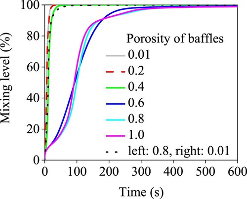
Figure 13. Velocity contours of Type 2 at $t$ = 600 s with baffles implemented on the left and right, the baffle length is 15 mm: (a) 0.2 porosity; (b) 0.8 porosity, (c) 0.8 porosity for the left one and 0.01 porosity for the right one.

5. Conclusions

In order to study the mixing behavior of SERs, especially to explore SERs with potential industrial applications, numerical simulations were performed and two basic motion types were considered. The mixing of the tracer (passive scalar) and the test fluid in 2D closed SERs was simulated using a species transport model. A dynamic mesh method was successfully utilized to handle the moving boundaries of the SERs. The mixing efficiency under different conditions was quantified with the aim of improving the design of SERs. It was found that the aspect ratio has a great influence on the mixing time of an SER with Type 1 motion mode. As the aspect ratio increases, the mixing speed first decreases and then increases slightly, which is not monotonic. For the Type 2 motion mode, a relatively higher mixing efficiency could be observed at all aspect ratios and an increase of the aspect ratio has no obvious effect on the mixing level. More wavenumbers could contribute to better mixing for the Type 1 motion mode, while an opposite trend was identified for the Type 2 motion mode. Under the conditions investigated, even the worst mixing performance in the case of Type 2 was better than the best Type 1 case. Baffles have significant influence on mixing in the SER for both motion types. Baffles implemented on Location 2 (i.e. on moving walls) performed better than on Location 1. At Location 2, the longer the baffle was, the faster the mixing could be. While at Location 1, longer baffles introduce more disordered flows for the SER with the Type 1 motion mode but hindered convective mixing in the SER with the Type 2 motion mode. Baffles with lower porosity were able to offer stronger stirring effects, and hence gave better mixing. Hence, the following configurations are beneficial to achieving a high mixing level within an SER: wave-like symmetrical-contraction boundary motion with a low wavenumber, and the installation of long low-permeable baffles at the moving wall.

Preliminary simulation-based factor explorations of the bio-inspired SERs in this work provide a basis for upgrading SERs to have improved mixing performances. For instance, the benefits of baffles can inspire an optimized design of SERs that are currently unbaffled (Liu, Xiao, et al., 2018). However, the results presented in this work are limited to 2D rectangular SERs, it should be checked whether fluid flow and the shape of the flow systems can be neglected in the third dimension when trying to apply these results. In future, simulations of 3D SERs with more realistic and various geometries should be conducted. Moreover, the mixing of fluids with different rheological properties in SERs should be investigated, which may offer insights into the digestion process since the chyme is often non-Newtonian (Kong & Singh, 2008).

Nomenclature

Symbols

$C$	=	Local mass fraction of the species
$C_{\text{ideal}}$	=	Mass fraction of adequately mixed state
$C\left(t\right)$	=	Mass fraction in a certain cell at time $t$
$D_p$	=	Effective average diameter of solid grains in the porous media region (the region of baffles) (mm)
$D_m$	=	Mass diffusion coefficient for the tracer in the mixture (m2/s)
$d_{\text{mix}}\left(t\right)$	=	Parameter that indicates the mixing uniformity at time $t$
$d_{\text{mix}}\left(0\right)$	=	Zero time of $d_{mix}\left(t\right)$
$H$	=	Height of SER (mm)
$H_t$	=	Height of the initial tracer domain (mm)
$K$	=	Permeability (m2)
$L$	=	Length of SER (mm)
$L_b$	=	Length of the baffle (mm)
$L_t$	=	Length of the initial tracer domain (mm)
$N$	=	Wavenumbers of the moving boundary
$N_p$	=	Processor number
$N_x$	=	Grid numbers in the x-direction
$N_y$	=	Grid numbers in the y-direction
$N_{\text{z}}$	=	Grid numbers in the z-direction
$p$	=	Static pressure divided by density (m2/s2)
$r_{hl}$	=	Aspect ratio of SER
$S$	=	The area of the whole computing domain (mm2)
$s_{ij}$	=	Strain rate (s−1)
$t$	=	Physical time (s)
$T$	=	Period of the boundary movement (s)
$T_b$	=	Thickness of the baffle (mm)
$u_i$	=	Fluid velocity component i (m/s)
$u_j$	=	Fluid velocity component j (m/s)
$u_{pi}$	=	Velocity of the moving mesh (m/s)
$ϵ$	=	Normalized deformation amplitude
$\nu$	=	Kinematic viscosity of the fluid (m2/s)
${\tau }_{ij}$	=	Viscous stress tensor (m2/s2­)
$\varphi$	=	Local porosity
$\psi$	=	General variable
${\psi }_{\text{ref}}$	=	The reference value for the general variable
$\mathrm{\Omega }$	=	Dimensionless scalar that accounts for baffle regions

Acronyms

CFD	=	Computational Fluid Dynamics
PISO	=	Pressure-Implicit with Splitting of Operators
SER	=	Soft-Elastic Reactor

Disclosure statement

No potential conflict of interest was reported by the authors.

Additional information

Funding

This work was supported by the National Natural Science Foundation of China [Grant numbers 21676172, 21978184]; the National Key Research and Development Program of China (International S&T Cooperation Program, ISTCP) [No. 2016YFE0101200]; the Natural Science Foundation of Jiangsu Province [Grant number BK20170062]; the Priority Academic Program Development (PAPD) of Jiangsu Higher Education Institutions.

References

- Alokaily, S., Feigl, K., & Tanner, F. X. (2019). Characterization of peristaltic flow during the mixing process in a model human stomach. Physics of Fluids, 31(10), 103105. https://doi.org/https://doi.org/10.1063/1.5122665
- Blanco-Aguilera, R., Lara, J., Barajas, G., Tejero, I., & Diez-Montero, R. (2020). CFD simulation of a novel anaerobic-anoxic reactor for biological nutrient removal: Model construction, validation and hydrodynamic analysis based on OpenFOAM®. Chemical Engineering Science, 215, 115390. https://doi.org/https://doi.org/10.1016/j.ces.2019.115390
- Cabaret, F., Fradette, L., & Tanguy, P. A. (2008). New turbine impellers for viscous mixing. Chemical Engineering & Technology, 31(12), 1806–1815. https://doi.org/https://doi.org/10.1002/ceat.200800385
- Chen, L., Xu, Y., Fan, T., Liao, Z., Wu, P., Wu, X., & Chen, X. D. (2016). Gastric emptying and morphology of a ‘near real’ in vitro human stomach model (RD-IV-HSM). Journal of Food Engineering, 183, 1–8. https://doi.org/https://doi.org/10.1016/j.jfoodeng.2016.02.025
- Chen, X. D. (2016). Scoping biology-inspired chemical engineering. Chinese Journal of Chemical Engineering, 24(1), 1–8. https://doi.org/https://doi.org/10.1016/j.cjche.2015.07.009
- Chen, X. D., & Liu, M. (2015). Material preparation and procedures for making a soft-elastic reactor and the methods for mixing in this reactor (Patent No. CN104841299A[P].
- Chen, X. D., & Yoo, J. Y. (2006). Food engineering as an advancing branch of chemical engineering. International Journal of Food Engineering, 2(2), 88–91. https://doi.org/https://doi.org/10.2202/1556-3758.1100
- Coppens, M. O. (2012). A nature-inspired approach to reactor and catalysis engineering. Current Opinion in Chemical Engineering, 1(3), 281–289. https://doi.org/https://doi.org/10.1016/j.coche.2012.03.002
- Delaplace, G., Gu, Y., Liu, M., Jeantet, R., Xiao, J., & Chen, X. D. (2018). Homogenization of liquids inside a new soft elastic reactor: Revealing mixing behavior through dimensional analysis. Chemical Engineering Science, 192, 1071–1080. https://doi.org/https://doi.org/10.1016/j.ces.2018.08.023
- Delaplace, G., Liu, M., Jeantet, R., Xiao, J., & Chen, X. D. (2020). Predicting the mixing time of soft elastic reactors: Physical models and empirical correlations. Industrial & Engineering Chemistry Research, 59(13), 6258–6268. https://doi.org/https://doi.org/10.1021/acs.iecr.9b06053
- Deng, R., Selomulya, C., Wu, P., Woo, M. W., Wu, X., & Chen, X. D. (2016). A soft tubular model reactor based on the bionics of a small intestine–starch hydrolysis. Chemical Engineering Research & Design, 112, 146–154. https://doi.org/https://doi.org/10.1016/j.cherd.2016.06.005
- Ferrua, M. J., & Singh, R. P. (2010). Modeling the fluid dynamics in a human stomach to gain insight of food digestion. Journal of Food Science, 75(7), R151–R162. https://doi.org/https://doi.org/10.1111/j.1750-3841.2010.01748.x
- Ferziger, J. H., Perić, M., & Street, R. L. (2002). Computational methods for fluid dynamics (Vol. 3). Springer.
- Gao, T., Wang, Y., Pang, Y., & Cao, J. (2016). Hull shape optimization for autonomous underwater vehicles using CFD. Engineering Applications of Computational Fluid Mechanics, 10(1), 599–607. https://doi.org/https://doi.org/10.1080/19942060.2016.1224735
- Hashimoto, S., Natami, K., & Inoue, Y. (2011). Mechanism of mixing enhancement with baffles in impeller-agitated vessel, part I: A case study based on cross-sections of streak sheet. Chemical Engineering Science, 66(20), 4690–4701. https://doi.org/https://doi.org/10.1016/j.ces.2011.06.032
- Hitimana, E., Fox, R. O., Hill, J. C., & Olsen, M. G. (2019). Experimental characterization of turbulent mixing performance using simultaneous stereoscopic particle image velocimetry and planar laser-induced fluorescence. Experiments in Fluids, 60(2), 28. https://doi.org/https://doi.org/10.1007/s00348-018-2669-y
- Ji, H., Hu, J., Zuo, S., Zhang, S., Li, M., & Nie, S. (2021). In vitro gastrointestinal digestion and fermentation models and their applications in food carbohydrates. Critical Reviews in Food Science and Nutrition, 1–23. https://doi.org/https://doi.org/10.1080/10408398.2021.1884841
- Kong, F., & Singh, R. (2008). Disintegration of solid foods in human stomach. Journal of Food Science, 73(5), R67–R80. https://doi.org/https://doi.org/10.1111/j.1750-3841.2008.00766.x
- Levy, A., & Kalman, C. J. (2001). Handbook of conveying and handling of particulate solids. Elsevier.
- Li, C., & Jin, Y. (2021). A CFD model for investigating the dynamics of liquid gastric contents in human-stomach induced by gastric motility. Journal of Food Engineering, 296, 110461. https://doi.org/https://doi.org/10.1016/j.jfoodeng.2020.110461
- Li, C., Xiao, J., Chen, X. D., & Jin, Y. (2021). Mixing and emptying of gastric contents in human-stomach: A numerical study. Journal of Biomechanics, 118, 110293. https://doi.org/https://doi.org/10.1016/j.jbiomech.2021.110293
- Li, C., Xiao, J., Zhang, Y., & Chen, X. D. (2019). Mixing in a soft-elastic reactor (SER): A simulation study. The Canadian Journal of Chemical Engineering, 97(3), 676–686. https://doi.org/https://doi.org/10.1002/cjce.23351
- Li, C., Yu, W., Wu, P., & Chen, X. D. (2020). Current in vitro digestion systems for understanding food digestion in human upper gastrointestinal tract. Trends in Food Science & Technology, 96, 114–126. https://doi.org/https://doi.org/10.1016/j.tifs.2019.12.015
- Li, Z., Zhu, L., Zhang, W., Zhan, X., & Gao, M. (2020). New dynamic digestion model reactor that mimics gastrointestinal function. Biochemical Engineering Journal, 154, 107431. https://doi.org/https://doi.org/10.1016/j.bej.2019.107431
- Liu, C., Xiang, C., Yan, Q., Wei, W., Watson, C., & Wood, H. G. (2019). Development and validation of a CFD based optimization procedure for the design of torque converter cascade. Engineering Applications of Computational Fluid Mechanics, 13(1), 128–141. https://doi.org/https://doi.org/10.1080/19942060.2018.1562383
- Liu, M., Xiao, J., & Chen, X. D. (2018). A soft-elastic reactor inspired by the animal upper digestion tract. Chemical Engineering & Technology, 41(5), 1051–1056. https://doi.org/https://doi.org/10.1002/ceat.201600617
- Liu, M., Zou, C., Xiao, J., & Chen, X. D. (2018). Soft-elastic bionic reactor. CIESC Journal, 69(1), 414–422. https://doi.org/https://doi.org/10.11949/j.issn.0438-1157.20171120
- Mosavi, A., Shamshirband, S., Salwana, E., Chau, K.-W., & Tah, J. H. (2019). Prediction of multi-inputs bubble column reactor using a novel hybrid model of computational fluid dynamics and machine learning. Engineering Applications of Computational Fluid Mechanics, 13(1), 482–492. https://doi.org/https://doi.org/10.1080/19942060.2019.1613448
- Nakashima, Y. (2000). Effects of clay fraction and temperature on the H2O self-diffusivity in hectorite gel: A pulsed-field-gradient spin-echo nuclear magnetic resonance study. Clays and Clay Minerals, 48(6), 603–609. https://doi.org/https://doi.org/10.1346/CCMN.2000.0480602
- Nield, D. A., & Bejan, A. (2006). Convection in porous media (Vol. 3). Springer.
- Schetz, J. A., & Fuhs, A. E. (1999). Fundamentals of fluid mechanics. John Wiley & Sons.
- Shamshirband, S., Babanezhad, M., Mosavi, A., Nabipour, N., Hajnal, E., Nadai, L., & Chau, K.-W. (2020). Prediction of flow characteristics in the bubble column reactor by the artificial pheromone-based communication of biological ants. Engineering Applications of Computational Fluid Mechanics, 14(1), 367–378. https://doi.org/https://doi.org/10.1080/19942060.2020.1715842
- Wu, P., & Chen, X. D. (2020). On designing biomimic in vitro human and animal digestion track models: Ideas, current and future devices. Current Opinion in Food Science, 35, 10–19. https://doi.org/https://doi.org/10.1016/j.cofs.2019.12.004
- Xiao, J., Zou, C., Liu, M., Zhang, G., Delaplace, G., Jeantet, R., & Chen, X. D. (2018). Mixing in a soft-elastic reactor (SER) characterized using an RGB based image analysis method. Chemical Engineering Science, 181, 272–285. https://doi.org/https://doi.org/10.1016/j.ces.2018.02.019
- Zha, J., Zou, S., Hao, J., Liu, X., Delaplace, G., Jeantet, R., Dupont, D., Wu, P., Chen, X. D., & Xiao, J. (2021). The role of circular folds in mixing intensification in the small intestine: A numerical study. Chemical Engineering Science, 229, 116079. https://doi.org/https://doi.org/10.1016/j.ces.2020.116079
- Zhang, X., Liao, Z., Wu, P., Chen, L., & Chen, X. D. (2018). Effects of the gastric juice injection pattern and contraction frequency on the digestibility of casein powder suspensions in an in vitro dynamic rat stomach made with a 3D printed model. Food Research International, 106, 495–502. https://doi.org/https://doi.org/10.1016/j.foodres.2017.12.082
- Zhang, Y. J., Wang, J. J., Gu, X. P., Feng, L. F., & Wu, B. (2016). CFD simulation of an agitated gas-fluidized bed: Effects of particle–particle restitution coefficient on the hydrodynamics. Chemical Engineering Research & Design, 111, 353–361. https://doi.org/https://doi.org/10.1016/j.cherd.2016.05.021
- Zou, J., Xiao, J., Zhang, Y., Li, C., & Chen, X. D. (2020). Numerical simulation of the mixing process in a soft elastic reactor with bionic contractions. Chemical Engineering Science, 220, 115623. https://doi.org/https://doi.org/10.1016/j.ces.2020.115623