Prediction of daily water level using new hybridized GS-GMDH and ANFIS-FCM models

Abstract

Accurate prediction of water level (WL) is essential for the optimal management of different water resource projects. The development of a reliable model for WL prediction remains a challenging task in water resources management. In this study, novel hybrid models, namely, Generalized Structure-Group Method of Data Handling (GS-GMDH) and Adaptive Neuro-Fuzzy Inference System with Fuzzy C-Means (ANFIS-FCM) were proposed to predict the daily WL at Telom and Bertam stations located in Cameron Highlands of Malaysia. Different percentage ratio for data division i.e. 50%–50% (scenario-1), 60%–40% (scenario-2), and 70%–30% (scenario-3) were adopted for training and testing of these models. To show the efficiency of the proposed hybrid models, their results were compared with the standalone models that include the Gene Expression Programming (GEP) and Group Method of Data Handling (GMDH). The results of the investigation revealed that the hybrid GS-GMDH and ANFIS-FCM models outperformed the standalone GEP and GMDH models for the prediction of daily WL at both study sites. In addition, the results indicate the best performance for WL prediction was obtained in scenario-3 (70%–30%). In summary, the results highlight the better suitability and supremacy of the proposed hybrid GS-GMDH and ANFIS-FCM models in daily WL prediction, and can, serve as robust and reliable predictive tools for the study region.

KEYWORDS:

• Water level prediction
• hybrid models
• GEP
• GMDH
• Cameron highland

1. Introduction

Prediction of river water level is a critical process in river discharge estimation and it is required for better water resources management (Dingman & Bjerklie, 2005; Tsujikura et al., 2016; Vachtman & Laronne, 2014). The accurate prediction of a river water level improves flood prediction systems and can act as a warning alarm for early decision-making and planning to reduce the effect of flood events which is considered as one of the most damaging natural hazards on life and property (Hettiarachchi & Thilakumara, 2014; Morales-Pinzón et al., 2015; Tsujikura et al., 2016; Xu et al., 2019). In Malaysia, floods and flash floods are often happened due to prolonged heavy rainfall; however, the possibility of floods may increase as a result of climate change and global warming (Arbain & Wibowo, 2012; Buslima et al., 2018; Suri et al., 2014). To deal with the flood phenomena, three categories of critical river water levels have been introduced by the Department of Irrigation and Drainage (DID) Malaysia, namely, normal, alert, and danger levels (Gasim et al., 2007). The three categories have been identified by analyzing the characteristics of floods in Malaysia, such as water level, peak discharge, inundated area, the volume of flow, and flood duration, for many years.

Water level prediction in rivers is usually conducted using empirical models. These empirical models are developed based on accumulating long-time-series data using in situ sensors that are expensive, hard to maintain, and available in specific areas (Rigos et al., 2020). However, as per (Hettiarachchi & Thilakumara, 2014) prediction of river water level using non-linear models that includes many environmental parameters (e.g. catchment area and flow rates) imperfectly agreed with the realistic observation data; this may due to the complex nature of the dynamic and rapidly water level fluctuations or due to ignoring some important parameters in the theory (See & Openshaw, 1999). Moreover, modeling these complex processes by differential equations has little use in practice as it results in complex, time-consuming, and mathematically intractable non-linear models.

Soft computing techniques have successfully used in the last three decades to solve different complex hydrological problems (Daliakopoulos et al., 2005; Ehteram et al., 2021; Hadi et al., 2019; Kaloop et al., 2017; Malik et al., 2020b; Parsaie et al., 2015; Sammen et al., 2017; Singh et al., 2018; Tikhamarine et al., 2020c; Yaseen et al., 2020b; Young et al., 2015). For water level prediction, several techniques have been used such as Artificial Neural Networks (ANN) (Alvisi et al., 2006), Autoregressive Integrated Moving Average (ARIMA) (Reza et al., 2018; Sihag et al., 2020; Xu et al., 2019), and Support Vector Machine (SVM) (Khan & Coulibaly, 2006; Liong & Sivapragasam, 2002). These models have been applied for flow and water level prediction of some rivers in Malaysia, such as Muda River, Kedah (Khairuddin et al., 2019), Dungun River, Terengganu (Gasim et al., 2007), Langat River, Selangor (Toriman et al., 2009). Evaluation of soft computing performance conducted by Firat (2008), Toriman et al. (2009), and Khairuddin et al. (2019) acknowledged superiority over statistical and time series methods for flood forecasting. Besides, the soft computing/ machine learning (ML) models received several practical applications in diverse fields like the prediction of solar radiation (Qin et al., 2018; Wang et al., 2016, 2017b), evaporation modeling (Adnan et al., 2019; Ashrafzadeh et al., 2020; Malik et al., 2017, 2018; Wang et al., 2017a, 2017c), rainfall-runoff forecasting (Malik et al., 2020b; Singh et al., 2018; Tikhamarine et al., 2020c), reference evapotranspiration estimation (Malik et al., 2019a; Mohamadi et al., 2020; Tikhamarine et al., 2019, 2020a, 2020b), meteorological and hydrological drought prediction (Malik et al., 2019c, 2020a, 2021a, 2021b, 2021c; Malik & Kumar, 2020), and simulation of seepage flow through embankment dam (Rehamnia et al., 2021).

Moreover, a comparison among ANN, ARMA (Auto-regressive Moving Average), and SVM models that were conducted by Lin et al. (2006) revealed that the SVM model can give a more accurate prediction of long-term flow discharges than the others. A comprehensive review of the applications of genetic programming (GP) in the analysis of water resources systems was conducted by Mohammad-Azari et al. (2020). The review indicates the capability and superiority of the model for solving a wide variety of water-related problems such as modeling rainfall-runoff, streamflow, sedimentation, flood, evaporation, water quality, water demand, and water distribution systems. Moosavi et al. (2017) evaluated the performance of GMDH and wavelet-GMDH models for daily runoff forecasting from Darian-Chay, Ghale-Chay, and Lilan-Chay Rivers in East Azerbaijan (Iran). The evaluation indicates that the performance of the GMDH model was efficiently enhanced when the wavelet-based analyzed data was added to the model to deal with the non- stationarities in the data.

In this study, two hybrid models, namely, Generalized Structure-Group Method of Data Handling (GS-GMDH) and Adaptive Neuro-Fuzzy Inference System with Fuzzy C-Means (ANFIS-FCM) were developed by using data obtained from two water level stations located in Perak River, Malaysia. The study also compared the efficiency and performance of the hybrid models (i.e. GS-GMDH and ANFIS-FCM) with two standalone models, namely, the Gene Expression Programming (GEP) and Group Method of Data Handling (GMDH) through statistical indicators and graphical interpretation. The results of this study promise better accuracy of the hybrid GS-GMDH and ANFIS-FCM models in river water level prediction.

2. Methodology and dataset

2.1. Study area

Cameron Highlands is the smallest region in the province of Pahang Darul Makmur and offers its fringes with the territory of Kelantan and Perak, in the north and west, respectively. It is situated in the Main Range (Banjaran Titiwangsa) between 4° 27′ 53^″ N – 4° 32′ 39^″ N and 101° 23′ 10^″ E – 101° 25′ 25^″ E. The region of Cameron Highlands with an expected region of 71,218 hectares is hilly, extending from 300 m at the stream valleys on the eastern limit to 210 m (Gunung Irau) on the western boundary. The most elevated point open by street in Peninsular Malaysia, Gunung Brinchang (2031 m), is one of the significant tops in Cameron Highlands, side from Gunung Swettenham (1961 m), Gunung Siku (1916 m), Gunung Berembun (1840 m), Gunung Cantik (1802 m) and Gunung Jasar (1704 m). About 75% of the area of the provenance is situated above 1000 m heights. The examination zone falls within Cameron Highlands Districts arranged at Pahang Darul Makmur, which the region assessed to be 712 km². Its temperature falls not more than 25°C and is broadly known as an uneven region with horticultural practices (Eisakhani & Malakahmad, 2009). Cameron Highlands is comprised of three significant catchments of Bertam, Telom, and Lemoi as shown in Figure 1. Bertam comprises five main sub-catchments which are Habu, Ringlet, Lembah Bertam, Tanah Rata, and Brinchang. While, Tringkap, Kampung Raja, and Kuala Terla are the sub-catchments in Telom. Cameron Highlands gets normal yearly precipitation of 2800 mm and normally 2 out of 3 days is raining (Tan & Beh, 2015). Therefore, almost every day precipitation could be felt in Cameron Highlands. The details of the station are organized in Table 1. For modeling the water level, daily data from January 2009 to August 2014 was used for Telom at Batu station, and data from January 2009 to March 20016 was used for Bertam at Rabinson Falls Intake station. Table 2 summarizes statistical parameters i.e. Max. = maximum, Min. = Minimum, SD = standard deviation, Skew = Skewness, Q1, Q2, and Q3 = first, second and third quartiles of WL at both stations.

Figure 1. Location map of study basin (Nasidi et al., 2021).

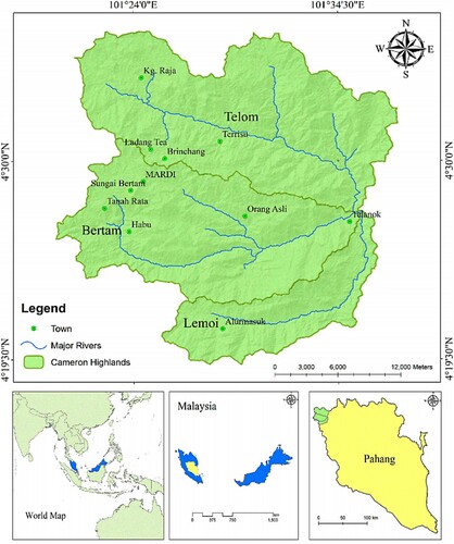
Table 1. List of water level stations with their geographical coordinates.

No.	Station No.	Station Name	Longitude (E)	Latitude (N)
1	6002	Telom at Batu 49	101° 25′ 25^″	4° 32′ 39^″
2	6003	Bertam at Rabinson Falls Intake	101° 23′ 10^″	4° 27′ 53^″

Table 2. The statistical characteristics of two stations.

Station	Mean (m)	Max. (m)	Min. (m)	SD	Skew	Q1	Q2	Q3
Telom	670	1469	399	153.26	1.467	566	643	735
Bertam	391	786	241	82.79	0.937	332	377	435

2.2. Gene expression programming (GEP)

GEP was initially introduced by Ferreira (2002). It is a generated technique with the base of genetic algorithms (GA) and has been broadly adopted in recent investigations (Ebtehaj et al., 2015a; Ferreira, 2002). The PC program of GEP is encoded in linear chromosomes, which are then explained into trees term (Shabani et al., 2018). A systematic diagram of GEP appears in Figure 2. The initial step is to create the underlying population, which occurs with subjective births of chromosomes. Then the chromosomes are converted to expression trees (ETs) that are analyzed by performance measures to shows the solubility of delivered ETs. If the outcomes convince the performance measures criteria, population producing stops, and if the outcomes are not agreeable, the system redeveloped with some improvement to make generation with improved value, and this procedure happens until the best outcomes are accomplished. For additional clarification about GEP, readers and researchers are referred to (Ferreira, 2006; Kiafar et al., 2017). According to that, there is no certain method to find the optimum values of the GEP parameters, the optimum values of the GEP parameters for each station were found through a trial-and-error process (Azimi et al., 2017). The most optimum values of the GEP parameters for each station are provided in Table 3.

Figure 2. Description of GEP model.

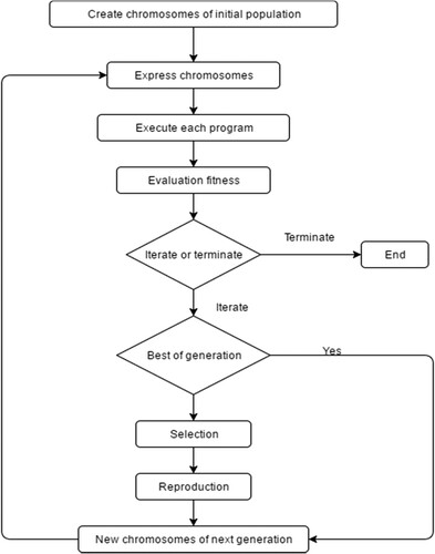
Table 3. The most optimum values of the GEP parameters.

	Telom station	Bertam station
Parameter	Setting
Number of chromosomes	50	50
Head size	10	10
Number of genes	5	3
Linking function	Addition	Addition
Fitness function	RRSE	RRSE
Mutation	0.014	0.01
Inversion	0.15	0.15
IS Transportation	0.15	0.15
RIS Transportation	0.15	0.15
One-point recombination	0.70	0.90
Two-point recombination	0.70	0.90
Gene recombination	0.20	0.10
Gene transposition	0.20	0.10

Note: RRSE = root relative squared error.

2.3. Group method of data handling (GMDH)

Ivakhnenko (1971) initially proposed the GMDH method. It’s practical in different sections for deep learning and science detection and is applied in several fields as forecasting, pattern recognition, and optimization. Analogical GMDH algorithms present the feasibility to discover automatically interrelations in data, to obtain the best structure of model or network, and to enhance the accuracy of existing algorithms. GMDH is containing numerous algorithms for the solution of various types of problems including clusterization, parametric, and probability algorithms. This method is relying on the sorting-out of gradually complex models and chooses the superlative solution via the lowest of outside criterion features. Generally, this method has numerous inputs and one output, which is a subset of elements of the base function (Madala & Ivakhnenko, 2019). To obtain the superior solution this model considers a variety of elements subsets of the initial function (Madala & Ivakhnenko, 2019) known as partial models. Least-squares techniques are used to find the coefficients of these models. GMDH algorithms gently enhance the number of incomplete model elements and discover a model structure with optimal complications represented via the lowest value of an outside criterion. This method is known as the self-organization of models (Schmidhuber, 2015): (1) $\begin{array}{rl}Y\left(x_1,\dots x_n\right)& ={\alpha }_0+\sum _{i=1}^m{\alpha }_i{f}_i\end{array}$(1) (2) $\begin{array}{rl}Y\left(x_1,\dots x_n\right)& ={\alpha }_0+\sum _{i=1}^n{\alpha }_i{x}_i+\sum _{i=1}^n\sum _{j=i}^n{\alpha }_{ij}{x}_{i{x}_j}\\ & +\sum _{i=1}^n\sum _{j=i}^n\sum _{k=j}^n{\alpha }_{ijk}{x}_i{x}_j{x}_k+\dots \end{array}$(2) where $Y\left(x_1,\dots x_n\right)$ represent the input content and $n$ the number of input variables. Also, $\alpha \left({\alpha }_1,\dots {\alpha }_n\right)$ coefficients are acquired via regression techniques for each couple of $x_i\text{and}{x}_j$ input variables (Farlow, 1981). Hence, the GMDH algorithm uses various second-degree polynomials.

2.4. Generalized structure-group method of data handling (GS-GMDH)

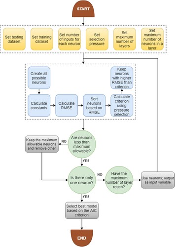
The standard GMDH model has few drawbacks that the low performance of this model in complex and nonlinear problems. In the present investigation, a novel encoding of GMDH has developed to increases the accuracy of the standard GMDH model. The main drawback of this model is the utilize of only two parameters as inputs for every neuron. In standard GMDH models, the input variables of every neuron are chosen from neighboring neurons. In the present study, a new generalized structure of the GMDH algorithm (GS-GMDH) model was developed to decrease the drawbacks of the standard GMDH model. The introduced new method decreases the limitations available in the standard GMDH algorithm. In GS-GMDH, the proposed neurons can be consisting of 2 or 3 input variables. Moreover, the polynomials are considered as second and third order. Besides, the input of every neuron can be chosen from both neighboring and non-neighboring layers. The most favorable structure of GS-GMDH (Figure 3) is obtained based on the Akaike Information Criterion (AIC) as follows (Ebtehaj et al., 2015b): (3) $\text{AIC}=n\ast \log \left(\text{MSE}\right)+2\left(N+1\right)$(3) where N is the number of neurons in the model, n is the number of samples, and MSE is the mean square error.

Figure 3. The flowchart of the proposed GS-GMDH model.

2.5. Adaptive neuro-fuzzy inference system (ANFIS)

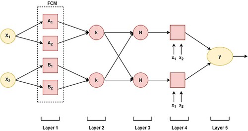
The adaptive neuro-fuzzy inference system (ANFIS) is an amalgamation of ANN and fuzzy logic (FL) for developing non-linear problems and initially, it was developed by Jang et al. IF-THEN fuzzy rules are utilized in model development by ANFIS (Sobhani et al., 2010; Yuan et al., 2014). It draws advantages of both ANN and FL. It could successfully be used where ordinary traditional techniques fail or too weighty (Vakhshouri & Nejadi, 2018). Shape and number of membership functions (MFs) are significant parameters in ANFIS to generate a model with the least error zone. Figure 4 display the structure of an ANFIS model having two input variables. For simplicity of illustration only two inputs p, q, and single target, y is considered in this figure.

Figure 4. The flowchart of the proposed ANFIS-FCM model.

2.6. Fuzzy C-means method (FCM)

The algorithm k-mean is one of the grouping algorithms, which is utilized broadly. This algorithm with unsupervised in large data sets is faced with limitations in preparing. To deal with the shortcoming, distinctive grouping algorithms are given. Fuzzy C-means clustering as an alternative technique is utilized (Kisi & Zounemat-Kermani, 2016). Fuzzy c-means (FCM) were presented by Bezdek et al. (1981), and improved by variables and dependent variables (target) specified in this stage are: (4) $\begin{array}{rl}{S}^1{M}_a& =\mu M_a\left(p\right),a=1,2\end{array}$(4) (5) $\begin{array}{rl}{S}^1{N}_a& =\mu N_a\left(q\right),a=1,2\end{array}$(5) where $p$ and $q$ are crisp inputs, and $M_a$ and $N_a$ are fuzzy set, low, medium, high-class size membership functions are applied, which could any shape such as triangular, trapezoidal, bell-shaped, Gaussian function, etc. (Cai et al., 2007). In Fuzzy clustering, designs in clusters with common are classified, and a pattern can appertain multiple clusters with an alternate proportion. In the FCM algorithm, designs are blocked to the C cluster, truth be told, the quantity of clusters (C) is indicated prior, yet the focal point of the cluster is chosen haphazardly. The level of membership for each example as indicated by the membership function is determined by the focal point of each cluster. The goal of the FCM algorithm is to discover a group that the likeness between designs inside various clusters is minimized. One of the primary benefits of the FCM technique is that in this approach, every data point is related to at least two clusters. The FCM cluster center utilizes the minimization of the objective function, which is considered as the squared separation between each group center and information point and is weighted by its memberships.

2.7. Performance indicators

The accuracy of the hybrid (i.e. GS-GMDH and ANFIS-FCM) and standalone (i.e. GMDH and GEP) models developed for water level prediction at both study stations were evaluated by using four performance or statistical indicators i.e. Root Mean Square Error (RMSE) (Malik et al., 2019b; Pham et al., 2021; Sammen et al., 2020), Nash-Sutcliffe efficiency (NSE) (Nash & Sutcliffe, 1970), Pearson Correlation Coefficient (PCC) (Adnan et al., 2019; Malik & Kumar, 2020), and Willmott Index (WI) (Willmott, 1981), and through graphical inspection (time-variation plot, scatter plot, box–whisker plot, and Taylor diagram). The RMSE, NSE, PCC, and WI are stated as (6) $\begin{array}{rl}\text{RMSE}& =\sqrt{\frac{1}{N}\sum _{i=1}^N{(\text{W}{\text{L}}_{\text{obs},i}-\text{W}{\text{L}}_{\text{pre},i})}^2}\end{array}$(6) (7) $\begin{array}{rl}\text{NSE}& =1-\left[\frac{\sum _{i=1}^N{(\text{W}{\text{L}}_{\text{obs},i}-\text{W}{\text{L}}_{\text{pre},i})}^2}{\sum _{i=1}^N{(\text{W}{\text{L}}_{\text{obs},i}-\overline{\text{W}{\text{L}}_{\text{obs }}})}^2}\right]\end{array}$(7) (8) $\begin{array}{rl}\text{PCC}& =\frac{\begin{array}{c}\sum _{i=1}^N\left(\text{W}{\text{L}}_{\text{obs},i}-\overline{\text{W}{\text{L}}_{\text{obs }}}\right)\\ \left(\text{W}{\text{L}}_{\text{pre},i}-\overline{\text{W}{\text{L}}_{\text{pre}}}\right)\end{array}}{\sqrt{\begin{array}{c}\sum _{i=1}^N{(\text{W}{\text{L}}_{\text{obs},i}-\overline{\text{W}{\text{L}}_{\text{obs }}})}^2\\ \sum _{i=1}^N{(\text{W}{\text{L}}_{\text{pre},i}-\overline{\text{W}{\text{L}}_{\text{pre}}})}^2\end{array}}}\end{array}$(8) (9) $\begin{array}{rl}\text{WI}& =1-\left[\frac{\sum _{i=1}^N{(\text{W}{\text{L}}_{\text{pre},i}-\text{W}{\text{L}}_{\text{obs},i})}^2}{\begin{array}{c}\sum _{i=1}^N(|\text{W}{\text{L}}_{\text{pre},i}-\overline{\text{W}{\text{L}}_{\text{obs }}}|\\ +|\text{W}{\text{L}}_{\text{obs},i}-\overline{\text{W}{\text{L}}_{\text{obs }}}|{)}^2\end{array}}\right]\end{array}$(9) where $N,\text{W}{\text{L}}_{\text{obs}},\text{W}{\text{L}}_{\text{pre}},\overline{\text{W}{\text{L}}_{\text{obs }}}$ and $\overline{\text{W}{\text{L}}_{\text{pre }}}$ are the data points, observed and predicted water level (WL) values for the ith observations, and mean of observed and predicted WL values, respectively. In general, if the applied models follow the criteria of higher values of NSE, PCC, and WI, and the lower value of RMSE designated a relatively better model for WL prediction at study stations. These four statistical indicators are commonly used performance indicators in assessing model performance, which has proven their values in previous studies. They are used together in this study because each of them has both advantages and disadvantages. The use of all four indicators will ensure that an all-around assessment can be made of the model performance.

3. Results and discussion

3.1. Performance assessment using statistical metrics

Four different machine learning techniques, namely, GEP, GMDH, GS-GMDH, and ANFIS-FCM were employed to predict the daily WL for two stations of Cameron Highlands in Malaysia. Table 4 present the results of the performance indices (i.e. RMSE, NSE, PCC, and WI) of the GEP, GMDH, GS-GMDH, and ANFIS-FCM models at Telom station during the validation period under three different scenarios. It is clear from Table 4 that the values of RMSE, NSE, PCC and WI found in the range of 87.340–88.552 m, 0.755–0.761, 0.869–0.873 and 0.923–0.927 for scenario-1, 84.203–84.704 m, 0.769–0.772, 0.878–0.879 and 0.929–0.931 for scenario-2, and 82.987–83.616 m, 0.763–0.767, 0.874–0.876 and 0.927–0.929 for scenario-3, respectively. According to the Table 4, the GS-GMDH models had better performance for all three scenarios, but optimal results yielded under scenario-3 with RMSE = 82.987 m, NSE = 0.767, PCC = 0.876 and WI = 0.929. Likewise, the GS-GMDH model follows the criteria of lower values of RMSE, and higher values of NSE, PCC, and WI for all three scenarios and designated the first (or highest) rank for water level prediction. Similarly, the ANFIS-FCM model closely follows the GS-GMDH model, while the GMDH and GEP models had similar performance for water level prediction for the Telom station.

Table 4. Performance indicators of hybrid and simple ML models at Telom station during the validation phase.

		Performance indicators
Scenario	Model	RMSE	NSE	PCC	WI
	GS-GMDH	87.340	0.761	0.873	0.927
	GMDH	88.053	0.757	0.871	0.925
	ANFIS-FCM	88.552	0.755	0.869	0.923
	GEP	88.224	0.756	0.870	0.924
Scenario-1 (50%–50%)
	GS-GMDH	84.203	0.772	0.879	0.931
	GMDH	84.573	0.770	0.878	0.929
	ANFIS-FCM	84.394	0.771	0.879	0.929
	GEP	84.704	0.769	0.878	0.929
Scenario-2 (60%–40%)
	GS-GMDH	82.987	0.767	0.876	0.929
	GMDH	83.131	0.766	0.876	0.928
	ANFIS-FCM	83.800	0.763	0.874	0.927
	GEP	83.616	0.764	0.875	0.927
Scenario-3 (70%–30%)

Similarly, Table 5 summaries the results of GEP, GMDH, GS-GMDH, and ANFIS-FCM models at Bertam station during validation phase. It was noted from Table 5 that the values of RMSE, NSE, PCC and WI found in the range 48.148–49.86 m, 0.646–0.656, 0.804–0.810 and 0.882–0.887 for scenario-1, 49.047–49.766 m, 0.639–0.649, 0.799–0.806 and 0.882–0.884 for scenario-2, and 48.143–49.041 m, 0.680–0.691, 0.825–0.832 and 0.895–0.900 for scenario-3, respectively. Besides, the GS-GMDH models had better performance for all three scenarios, but improved results produced under scenario-3 (RMSE = 48.143 m, NSE = 0.691, PCC = 0.832 and WI = 0.900).

Table 5. Performance indicators of hybrid and simple ML models at Bertam station during the validation phase.

		Performance indicators
Scenario	Model	RMSE	NSE	PCC	WI
	GS-GMDH	49.148	0.656	0.810	0.887
	GMDH	49.860	0.646	0.804	0.882
	ANFIS-FCM	49.379	0.653	0.808	0.885
	GEP	49.730	0.648	0.805	0.885
Scenario-1 (50%–50%)
	GS-GMDH	49.047	0.649	0.806	0.884
	GMDH	49.766	0.639	0.799	0.879
	ANFIS-FCM	49.197	0.647	0.805	0.884
	GEP	49.672	0.640	0.800	0.882
Scenario-2 (60%–40%)
	GS-GMDH	48.143	0.691	0.832	0.900
	GMDH	49.041	0.680	0.825	0.895
	ANFIS-FCM	48.379	0.688	0.830	0.899
	GEP	48.495	0.687	0.829	0.900
Scenario-3 (70%–30%)

Furthermore, the prediction accuracy of the GS-GMDH model improved by 0.81%, 1.37%, 1.00% in scenario-1; 0.44%, 0.23%, 0.59% in scenario-2, and 0.17%, 0.97%, 0.75% in scenario-3 with respect to RMSE over GMDH, ANFIS-FCM and GEP models at Telom station. Likewise, the prediction accuracy of the GS-GMDH model enhanced by 1.43%, 0.47%, 1.17% in scenario-1, 1.44%, 0.30%, 1.26% in scenario-2, and 1.83%, 0.49%, 0.73% in scenario-3 regarding the RMSE over GMDH, ANFIS-FCM and GEP models at Bertam station. Therefore, for the Telom and Bertam stations, the obtained results indicate that the best performance was attained under scenario-3 where the data was divided by 70% for the calibration and the remaining 30% for validating the models.

3.2. Performance assessment using graphical interpretation

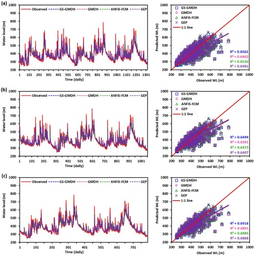
Besides the statistical assessment of the results, graphical methods have been widely used for model assessment. Accordingly, three different graphical methods namely temporal and scatter plots, Box–Whisker plot, and Taylor diagram were adopted in the study to assess the model performance graphically. Figures 5 and 6 illustrate the temporal and scatter plots of GS-GMDH, GMDH, ANFIS-FCM, and GEP models under scenario-1, scenario-2, and scenario-3 during the validation period at Telom and Bertam stations, respectively. As can see from these two figures that the GS-GMDH model had a higher value of the coefficient of determination: R² = 0.7619, 0.7724, and 0.7679 for scenario-1, scenario-2, and scenario-3 respectively at Telom station. Similarly, the high value of R² = 0.6562, 0.6494, and 0.6916 for scenario-1, scenario-2, and scenario-3, respectively was obtained when the GS-GMDH model was applied at Bertam station.

Figure 5. Comparison of observed and predicted WL values by GS-GMDH, GMDH, ANFIS-FCM, and GEP models under (a) scenario-1, (b) scenario-2, and (c) scenario-3 during validation period at Telom station.

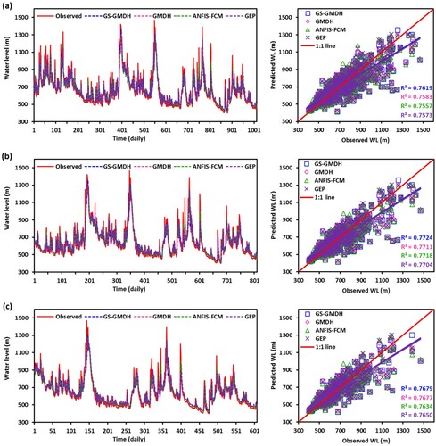
Figure 6. Comparison of observed and predicted WL values by GSGMDH, GMDH, ANFIS-FCM, and GEP models over (a) scenario-1, (b) scenario-2, and (c) scenario-3 during validation period at Bertam station.

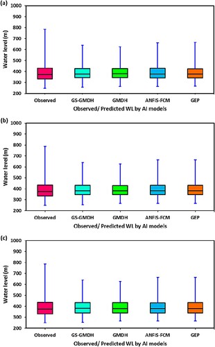
Furthermore, the performance of the GS-GMDH, GMDH, ANFIS-FCM, and GEP models in this study was evaluated by using the Box–Whisker plot. According to this diagram, it is easy to explain if there is any skew in the distribution of the data or there are any outliers. Figures 7 and 8 display the Box–Whisker plots for Telom and Bertam, respectively. In these figures, the distribution of the predicted values over the observed values during the validation period was explained. It was seen from the figures the distributional variation among predicted vs observed water level values were relatively minor. Therefore, the verdict based on performance measures (RMSE, NSE, PCC, and WI) and graphical inspection (coefficient of determination of regression line in scatter plots) showed the better water level prediction accuracy of the hybrid GS-GMDH model than the GMDH, ANFIS-FCM, and GEP models.

Figure 7. Box-Whisker plot of observed and predicted WL by GS-GMDH, GMDH, ANFIS-FCM, and GEP models in (a) scenario-1, (b) scenario-2, and (c) scenario-3 during validation period at Telom station.

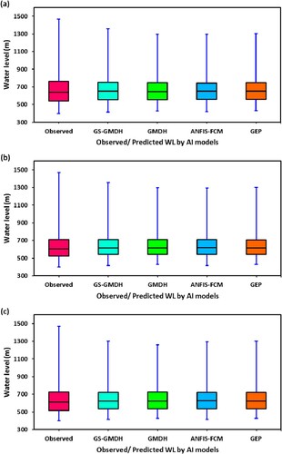
Figure 8. Box-Whisker plot of observed and predicted WL by GS-GMDH, GMDH, ANFIS-FCM, and GEP models in (a) scenario-1, (b) scenario-2, and (c) scenario-3 during validation period at Bertam station.

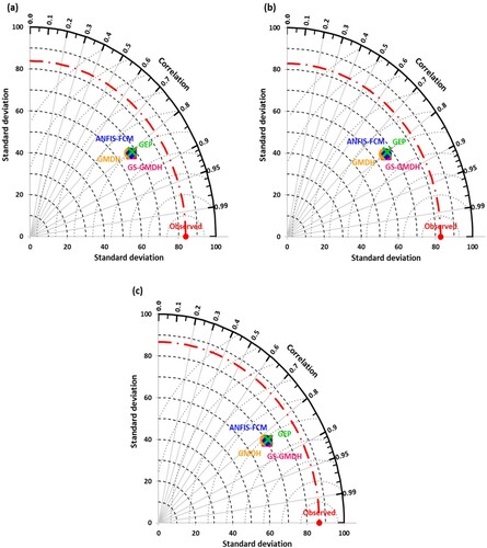
Likewise, the Taylor diagram (Taylor, 2001), an association of standard deviation, RMSE, and the correlation coefficient was employed to display the spatial variation of predicted water level using all four models in three different scenarios over the observed one in a single topology. Figures 9 and 10 demonstrate the Taylor diagram for the relative performance at Telom and Bertam sites, respectively. These diagrams clearly show the better performance of the GS-GMDH model for both stations. It is clear from Figures 9 and 10 that the obtained results by the GS-GMDH models are closer to the observed values of water level prediction and it has the superior performance as discussed before in the previous section.

Figure 9. Taylor diagram of GS-GMDH, GMDH, ANFIS-FCM, and GEP models under (a) scenario-1, (b) scenario-2, and (c) scenario-3 during validation phase at Telom station.

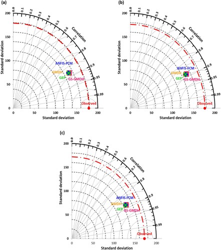
Figure 10. Taylor diagram of GSGMDH, GMDH, ANFIS-FCM, and GEP models under (a) scenario-1, (b) scenario-2, and (c) scenario-3 during validation phase at Bertam station.

The final equation of the GEP for both stations are provided as follow: (10) $\begin{array}{rl}WL\left(t\right)\mathrm{\_}Telom& =\left(\right(WL\left(t-3\right)-WL\left(t-1\right))\\ & /(-4.87/(\left(\right(WL\left(t-3\right)-WL\left(t-1\right))\\ & -WL\left(t-1\right)\left)/\right(WL\left(t-3\right)+9.44\left)\right)\left)\right)\\ & +\left(\right(\left(\right(\left(\right(WL\left(t-2\right)+WL\left(t-6\right))\\ & \ast -5.32\left)/WL\right(t-4\left)\right)\ast WL\left(t-2\right))\\ & /WL\left(t-5\right))-5.32)\\ & +\left(sqrt\left(WL\left(t-6\right)\right)+WL\left(t-1\right)\right)\\ & +\left(\right((8.82-(WL(t-3{)}^{\left(1/3\right)}\left)\right)\\ & \ast \left(sqrt\right(WL(t-1))\ast WL(t-1\left)\right))\\ & /WL(t-3))+((-1.61{)}^3)\end{array}$(10) (11) $\begin{array}{rl}\text{WL}\left(t\right)\mathrm{\_}\text{Bertam}& =2+\left(\right(\left(\right(\text{WL}\left(t-5\right)-\text{WL}\left(t-1\right))\\ & -\left(-0.56+\text{WL}\left(t-1\right)\right))\\ & +\left(\text{WL}\left(t-3\right)-\text{WL}\left(t-1\right)\right)\left)/8.88\right)\\ & +\left(\right(\left(\right(7.49+\text{WL}\left(t-3\right))\\ & +\left(\text{WL}\right(t-2)+7.49)\left)/\right(\left(\text{WL}\right(t-2)\\ & -\text{WL}\left(t-3\right))-\text{WL}(t-5\left)\right))\\ & +\text{WL}\left(t-1\right))\end{array}$(11)

The results of the current research were compared with existing studies on water level prediction by employing machine learning techniques. Altunkaynak (2019) predicted monthly WL in Lake Van, Tukey by employing the multilayer perceptron (MLP), wavelet-MLP (W-MLP), and MLP-ASA (additive season algorithm). Their prediction performance was evaluated using RMSE and NSE criteria. They found that the MLP-ASA model (RMSE = 3.550 cm, NSE = 0.992) outperformed the other models. Alizamir et al. (2020) employed a deep echo state network (DESN) to predict the monthly WL of lake Van (Turkey), and its outcomes were compared against the ANN, extreme learning machine (ELM), and regression tree (RT) based on RMSE, R², and NSE performance indicators. The investigation shows better performance of the DESN model with RMSE = 0.025 m, NSE = 0.998, and R² = 0.998 than the ANN, ELM, and RT models. Nhu et al. (2020) applied four decision tree-based algorithms i.e. M5 pruned (M5P), random forest (RF), RT, and reduced error pruning tree (REPT) for predicting the daily WL in Zrebar Lake, Iran during 2011–2017. These models were optimized with 70% data for training and 30% data for testing. Their performance was evaluated using RMSE, MAE, (mean absolute error), R², PBIAS (percent bias), and RSR (ratio of RMSE to standard deviation of observed data) indicators and graphical interpretation (Taylor and Box plots). They reported the M5P model produced better estimates (R² = 0.99, RMSE = 0.05 m, MAE = 0.01 m, NSE = 0.98, PBIAS = 0.00, RSR = 0.11) than the other models. Yaseen et al. (2020a) examined the comparative potential of the hybrid MLP-WOA (Whale Optimization Algorithm) model against the CCNN (Cascade Correlation Neural Network), SOM (Self Organizing Map), DTR (Decision Tree Regression), RFR (Random Forest Regression), and Classical MLP to predict the monthly WL of Van Lake, Turkey. The comparison demonstrates that the hybrid MLP-WOA models produced superior prediction (RMSE = 0.047 m, MAE = 0.035 m, NSE = 0.969, WI = 0.992, Legate McCabe’s Index: LMI = 0.836, and R²= 0.970) over other models during validation phase. Zhu et al. (2020) forecasted the monthly WL of 69 temperate lakes in Poland by utilizing Feed Forward Neural Network (FFNN), and Long Short-Term Memory (LSTM) models. Their finding reveals the better feasibility of FFNN and LSTM models in forecasting the monthly WL of the 69 lakes. Overall, the findings of the listed studies and current research confirm the superiority of ML models in predicting the daily/ monthly Lake water levels.

4. Conclusions

The present study has presented two new hybrid machine learning models, namely, generalized structure with GMDH algorithm (GS-GMDH) and adaptive neuro-fuzzy inference system with fuzzy C-means (ANFIS-FCM) for daily water level prediction at Telom, and Bertam stations positioned on Perak River in Malaysia. The performance of the hybrid models was compared with standalone models i.e. GEP and GMDH. To meet the objectives, the daily water level data of two stations for the Cameron Highlands in Malaysia were used. In addition, three different percentage ratios were used to divide the data for calibration and validation sets which include 50%–50%, 60%–40%, and 70%–30%, respectively. The results of the analysis reveal that the performance of the GMDH model could be enhanced with a new general structure (GS-GMDH) model. According to the best performance, the models were ordered as GS-GMDH > ANFIS-FCM > GEP > GMDH for both study locations. In addition, the results of the hybrid GS-GMDH model can be utilized to formulate the smart and truthful intelligent system for managing the water-related operations over the study sites.

Acknowledgements

The authors are grateful to the Tenaga Nasional Berhad (TNB) (Malaysia) for providing the original dataset and Universiti Tenaga Nasional (UNITEN) for providing the financial support for this study.

Disclosure statement

No potential conflict of interest was reported by the author(s).

References

- Adnan, R. M., Malik, A., Kumar, A, Parmar, K. S., Kisi, O. (2019). Pan evaporation modeling by three different neuro-fuzzy intelligent systems using climatic inputs. Arabian Journal of Geosciences, 12(19), 606. https://doi.org/https://doi.org/10.1007/s12517-019-4781-6
- Alizamir, M., Kisi, O., Kim, S., & Heddam, S. (2020). A novel method for lake level prediction: Deep echo state network. Arabian Journal of Geosciences, 13(18). https://doi.org/https://doi.org/10.1007/s12517-020-05965-9
- Altunkaynak, A. (2019). Predicting water level fluctuations in Lake Van using hybrid season-neuro approach. Journal of Hydrologic Engineering, 24(8), 04019021. https://doi.org/https://doi.org/10.1061/(asce)he.1943-5584.0001804
- Alvisi, S., Mascellani, G., Franchini, M., & Bárdossy, A. (2006). Water level forecasting through fuzzy logic and artificial neural network approaches. Hydrology and Earth System Sciences, 10 (1), 1–17. https://doi.org/https://doi.org/10.5194/hess-10-1-2006
- Arbain, S. H., & Wibowo, A. (2012). Time Series methods for water level forecasting of Dungun River in Terengganu Malaysia. Int J Eng Sci Technol, 4, 1803–1811.
- Ashrafzadeh, A., Malik, A., Jothiprakash, V., et al. (2020). Estimation of daily pan evaporation using neural networks and meta-heuristic approaches. ISH Journal of Hydraulic Engineering, 26(4), 421–429. https://doi.org/https://doi.org/10.1080/09715010.2018.1498754
- Azimi, H., Bonakdari, H., & Ebtehaj, I. (2017). A highly efficient gene expression programming model for predicting the discharge coefficient in a side weir along a trapezoidal canal. Irrigation and Drainage, 66(4), 655–666. https://doi.org/https://doi.org/10.1002/ird.2127
- Bezdek, J. C., Coray, C., Gunderson, R., & Watson, J. (1981). Detection and characterization of cluster substructure I. Linear structure: Fuzzy c -lines. SIAM Journal on Applied Mathematics, 40(2), 339–357. https://doi.org/https://doi.org/10.1137/0140029
- Buslima, F. S., Omar, R. C., Jamaluddin, T. A., & Taha, H. (2018). Flood and flash flood geo-hazards in Malaysia. International Journal of Engineering & Technology, 7(4.35), 760–764. https://doi.org/https://doi.org/10.14419/ijet.v7i4.35.23103
- Cai, W., Chen, S., & Zhang, D. (2007). Fast and robust fuzzy c-means clustering algorithms incorporating local information for image segmentation. Pattern Recognition, 40(3), 825–838. https://doi.org/https://doi.org/10.1016/j.patcog.2006.07.011
- Daliakopoulos, I. N., Coulibaly, P., & Tsanis, I. K. (2005). Groundwater level forecasting using artificial neural networks. Journal of Hydrology, 309(1–4), 229–240. https://doi.org/https://doi.org/10.1016/j.jhydrol.2004.12.001
- Dingman, S. L., & Bjerklie, D. M. (2005). Estimation of river discharge. Encycl Hydrol Sci John Wiley Sons.
- Ebtehaj, I., Bonakdari, H., Zaji, A. H., et al. (2015a). Gene expression programming to predict the discharge coefficient in rectangular side weirs. Applied Soft Computing, 35, 618–628. https://doi.org/https://doi.org/10.1016/j.asoc.2015.07.003
- Ebtehaj, I., Bonakdari, H., Zaji, A. H., et al. (2015b). GMDH-type neural network approach for modeling the discharge coefficient of rectangular sharp-crested side weirs. Engineering Science and Technology, an International Journal, 18(4), 746–757. https://doi.org/https://doi.org/10.1016/j.jestch.2015.04.012
- Ehteram, M., Ferdowsi, A., Faramarzpour, M., et al. (2021). Hybridization of artificial intelligence models with nature inspired optimization algorithms for lake water level prediction and uncertainty analysis. Alexandria Engineering Journal, 60(2), 2193–2208. https://doi.org/https://doi.org/10.1016/j.aej.2020.12.034
- Eisakhani, M., & Malakahmad, A. (2009). Water quality assessment of Bertam River and its tributaries in Cameron highlands. Malaysia. World Appl Sci J, 7, 769–776.
- Farlow, S. J. (1981). The GMDH algorithm of Ivakhnenko. The American Statistician, 35(4), 210. https://doi.org/https://doi.org/10.2307/2683292
- Ferreira, C. (2002). Gene expression programming in problem solving. Soft Computing and Industry.
- Ferreira, C. (2006). Gene Expression Programming Mathematical Modeling by an Artificial Intelligence.
- Firat, M. (2008). Comparison of artificial intelligence techniques for river flow forecasting. Hydrology and Earth System Sciences, 12(1), 123–139 https://doi.org/https://doi.org/10.5194/hess-12-123-2008
- Gasim, M. B., Adam, J. H., Toriman, M. E. H., et al. (2007). Coastal flood phenomenon in terengganu. Malaysia: Special Reference to Dungun. Res J Environ Sci, 1, 102–109. https://doi.org/https://doi.org/10.3923/rjes.2007.102.109
- Hadi, S. J., Abba, S. I., Sammen, S. S. H., et al. (2019). Non-linear input variable selection approach integrated with non-tuned data intelligence model for streamflow pattern simulation. IEEE Access, 7, 141533–141548. https://doi.org/https://doi.org/10.1109/ACCESS.2019.2943515
- Hettiarachchi, N., & Thilakumara, R. P. (2014). Water Level Forecasting and Flood Warning System A Neuro-Fuzzy Approach. International Conference in Video Image and Signal Processing, at India.
- Ivakhnenko, A. G. (1971). Polynomial theory of complex systems. IEEE Transactions on Systems, Man, and Cybernetics, SMC-1(4), 364–378. https://doi.org/https://doi.org/10.1109/TSMC.1971.4308320
- Kaloop, M. R., El-Diasty, M., & Hu, J. W. (2017). Real-time prediction of water level change using adaptive neuro-fuzzy inference system. Geomatics, Natural Hazards and Risk, 8(2), 1320–1332. https://doi.org/https://doi.org/10.1080/19475705.2017.1327464
- Khairuddin, N., Aris, A. Z., Elshafie, A., et al. (2019). Efficient forecasting model technique for river stream flow in tropical environment. Urban Water Journal, 16(3), 183–192. https://doi.org/https://doi.org/10.1080/1573062X.2019.1637906
- Khan, M. S., & Coulibaly, P. (2006). Application of support vector machine in lake water level prediction. Journal of Hydrologic Engineering, 11(3), 199–205. https://doi.org/https://doi.org/10.1061/(ASCE)1084-0699(2006)11:3(199)
- Kiafar, H., Babazadeh, H., Marti, P., et al. (2017). Evaluating the generalizability of GEP models for estimating reference evapotranspiration in distant humid and arid locations. Theoretical and Applied Climatology, 130, 377–389. https://doi.org/https://doi.org/10.1007/s00704-016-1888-5
- Kisi, O., & Zounemat-Kermani, M. (2016). Suspended sediment modeling using neuro-fuzzy embedded fuzzy c-means clustering technique. Water Resources Management, 30(11), 3979–3994 https://doi.org/https://doi.org/10.1007/s11269-016-1405-8
- Lin, J.-Y., Cheng, C.-T., & Chau, K.-W. (2006). Using support vector machines for long-term discharge prediction. Hydrological Sciences Journal, 51(4), 599–612. https://doi.org/https://doi.org/10.1623/hysj.51.4.599
- Liong, S. Y., & Sivapragasam, C. (2002). Flood stage forecasting with support vector machines. Journal of the American Water Resources Association, 38(1), 173–186. https://doi.org/https://doi.org/10.1111/j.1752-1688.2002.tb01544.x
- Madala, H. R., & Ivakhnenko, A. G. (2019). Inductive learning algorithms for complex systems modeling.
- Malik, A., & Kumar, A. (2020). Meteorological drought prediction using heuristic approaches based on effective drought index: A case study in uttarakhand. Arabian Journal of Geosciences, 13(1), 1–17. https://doi.org/https://doi.org/10.1007/s12517-020-5239-6
- Malik, A., Kumar, A., Ghorbani, M. A., et al. (2019a). The viability of co-active fuzzy inference system model for monthly reference evapotranspiration estimation: Case study of Uttarakhand State. Hydrology Research, 50(6), 1623–1644. https://doi.org/https://doi.org/10.2166/nh.2019.059
- Malik, A., Kumar, A., & Kisi, O. (2017). Monthly pan-evaporation estimation in Indian central Himalayas using different heuristic approaches and climate based models. Computers and Electronics in Agriculture, 143, 302–313. https://doi.org/https://doi.org/10.1016/j.compag.2017.11.008
- Malik, A., Kumar, A., & Kisi, O. (2018). Daily pan evaporation estimation using heuristic methods with Gamma test. Journal of Irrigation and Drainage Engineering, 144(9), 04018023. https://doi.org/https://doi.org/10.1061/(ASCE)IR.1943-4774.0001336
- Malik, A., Kumar, A., Kisi, O., & Shiri, J. (2019b). Evaluating the performance of four different heuristic approaches with Gamma test for daily suspended sediment concentration modeling. Environmental Science and Pollution Research, 26(22), 22670–22687. https://doi.org/https://doi.org/10.1007/s11356-019-05553-9
- Malik, A., Kumar, A., Rai, P., & Kuriqi, A. (2021a). Prediction of multi-scalar standardized precipitation index by using artificial intelligence and regression models. Climate, 9(2), 28. https://doi.org/https://doi.org/10.3390/cli9020028
- Malik, A., Kumar, A., Salih, S. Q., et al. (2020a). Drought index prediction using advanced fuzzy logic model: Regional case study over kumaon in India. PLoS One, 15(5), e0233280. https://doi.org/https://doi.org/10.1371/journal.pone.0233280
- Malik, A., Kumar, A., & Singh, R. P. (2019c). Application of heuristic approaches for prediction of hydrological drought using multi-scalar Streamflow drought index. Water Resources Management, 33(11), 3985–4006. https://doi.org/https://doi.org/10.1007/s11269-019-02350-4
- Malik, A., Tikhamarine, Y., Sammen, S. S., et al. (2021b). Prediction of meteorological drought by using hybrid support vector regression optimized with HHO versus PSO algorithms. Environmental Science and Pollution Research, 28(29), 39139–39158. https://doi.org/https://doi.org/10.1007/s11356-021-13445-0
- Malik, A., Tikhamarine, Y., Souag-Gamane, D., et al. (2020b). Support vector regression optimized by meta-heuristic algorithms for daily streamflow prediction. Stochastic Environmental Research and Risk Assessment, 34(11), 1755–1773. https://doi.org/https://doi.org/10.1007/s00477-020-01874-1
- Malik, A., Tikhamarine, Y., Souag-Gamane, D., et al. (2021c). Support vector regression integrated with novel meta-heuristic algorithms for meteorological drought prediction. Meteorology and Atmospheric Physics, 133(3), 891–909. https://doi.org/https://doi.org/10.1007/s00703-021-00787-0
- Mohamadi, S., Sammen, S. S., Panahi, F., et al. (2020). Zoning map for drought prediction using integrated machine learning models with a nomadic people optimization algorithm. Natural Hazards, 104(1), 537–579. https://doi.org/https://doi.org/10.1007/s11069-020-04180-9
- Mohammad-Azari, S., Bozorg-Haddad, O., & Loáiciga, H. A. (2020). State-of-art of genetic programming applications in water-resources systems analysis. Environ. Monit. Assess, 192, 73 (2020). https://doi.org/https://doi.org/10.1007/s10661-019-8040-9.
- Moosavi, V., Talebi, A., & Hadian, M. R. (2017). Development of a hybrid wavelet packet-group method of data handling (WPGMDH). Model for Runoff Forecasting. Water Resour Manag, 31(1), 43–59. https://doi.org/https://doi.org/10.1007/s11269-016-1507-3
- Morales-Pinzón, T., Céspedes-Restrepo, J. D., & Flórez-Calderón, M. T. (2015). Daily river level forecast based on the development of an artificial neural network case study in La Virginia-Risaralda. Revista Facultad de Ingeniería Universidad de Antioquia, 2015(76), 46–57. https://doi.org/https://doi.org/10.17533/udea.redin.n76a06
- Nash, J. E., & Sutcliffe, J. V. (1970). River flow forecasting through conceptual models part I – a discussion of principles. Journal of Hydrology, 10(3), 282–290. https://doi.org/https://doi.org/10.1016/0022-1694(70)90255-6
- Nasidi, N. M., Wayayok, A., Abdullah, A. F., et al. (2021). Dynamics of potential precipitation under climate change scenarios at Cameron highlands. SN Applied Sciences, 3(3), 334. https://doi.org/https://doi.org/10.1007/s42452-021-04332-x
- Nhu, V. H., Shahabi, H., Nohani, E., et al. (2020). Daily water level prediction of zrebar lake (Iran): A comparison between m5p, random forest, random tree and reduced error pruning trees algorithms. ISPRS International Journal of Geo-Information, 9(8), 479. https://doi.org/https://doi.org/10.3390/ijgi9080479
- Parsaie, A., Yonesi, H. A., & Najafian, S. (2015). Predictive modeling of discharge in compound open channel by support vector machine technique. Modeling Earth Systems and Environment, 1(1–2). https://doi.org/https://doi.org/10.1007/s40808-015-0002-9
- Pham, Q. B., Mohammadpour, R., Linh, N. T. T., et al. (2021). Application of soft computing to predict water quality in wetland. Environmental Science and Pollution Research, 28(1), 185–200. https://doi.org/https://doi.org/10.1007/s11356-020-10344-8
- Qin, W., Wang, L., Lin, A., et al. (2018). Comparison of deterministic and data-driven models for solar radiation estimation in China. Renew. Sustain. Energy Rev, 81(1), 579–594. https://doi.org/https://doi.org/10.1016/j.rser.2017.08.037
- Rehamnia, I., Benlaoukli, B., Jamei, M., et al. (2021). Simulation of seepage flow through embankment dam by using a novel extended Kalman filter based neural network paradigm: Case study of Fontaine Gazelles Dam, Algeria. Measurement, 176, 109219. https://doi.org/https://doi.org/10.1016/j.measurement.2021.109219
- Reza, M., Harun, S., & Askari, M. (2018). Streamflow forecasting in Bukit Merah Watershed by using Arima and Ann. Portal: Jurnal Teknik Sipil, 9(1), 18–26. https://doi.org/https://doi.org/10.30811/portal.v9i1.612.
- Rigos, A., Krommyda, M., Tsertou, A., & Amditis, A. (2020). A polynomial neural network for river’s water-level prediction. SN Applied Sciences, 2(4. https://doi.org/https://doi.org/10.1007/s42452-020-2328-9.
- Sammen, S. S., Ghorbani, M. A., Malik, A., Tikhamarine, Y., AmirRahmani, M., Al-Ansari, N., Chau, K. W., (2020). Enhanced artificial neural network with Harris hawks optimization for predicting scour depth downstream of ski-jump spillway. Applied Sciences, 10(15), 5160. https://doi.org/https://doi.org/10.3390/app10155160
- Sammen, S. S., Mohamed, T. A., Ghazali, A. H., El-Shafie, A. H., Sidek, L. M., (2017). Generalized regression neural network for prediction of peak outflow from dam breach. Water Resources Management, 31(1), 549–562. https://doi.org/https://doi.org/10.1007/s11269-016-1547-8
- Schmidhuber, J. (2015). Deep learning in neural networks: An overview. Neural Networks, 61, 85–117. https://doi.org/https://doi.org/10.1016/j.neunet.2014.09.003
- See, L., & Openshaw, S. (1999). Applying soft computing approaches to river level forecasting. Hydrological Sciences Journal, 44(5), 763–778. https://doi.org/https://doi.org/10.1080/02626669909492272
- Shabani, S., Candelieri, A., Archetti, F., & Naser, G. (2018). Gene expression programming coupled with unsupervised learning: A two-stage learning process in multi-scale, short-termwater demand forecasts. Water, 10(2), 142. https://doi.org/https://doi.org/10.3390/w10020142
- Sihag, P., Al-Janabi, A. M. S., Alomari, N. K., & Ghani, A. A. (2020). Tree regression for river discharge estimation: Application to the Baitarani River Basin. Modeling Earth Systems and Environment. https://doi.org/https://doi.org/10.1007/s40808-020-01045-9
- Singh, A., Malik, A., Kumar, A., & Kisi, O. (2018). Rainfall-runoff modeling in hilly watershed using heuristic approaches with gamma test. Arabian Journal of Geosciences, 11(1), 1–12. https://doi.org/https://doi.org/10.1007/s12517-018-3614-3
- Sobhani, J., Najimi, M., Pourkhorshidi, A. R., & Parhizkar, T. (2010). Prediction of the compressive strength of no-slump concrete: A comparative study of regression, neural network and ANFIS models. Construction and Building Materials, 24(5), 709–718. https://doi.org/https://doi.org/10.1016/j.conbuildmat.2009.10.037
- Suri, S., Ahmad, F., Yahaya, A. S., Mokhtar, Z. A., Halim, M. H., et al. (2014). Climate change impact on water level in Peninsular Malaysia. 4, 228–232. https://doi.org/https://doi.org/10.5923/c.jce.201402.39
- Tan, K. W., & Beh, W. C. (2015). Water quality monitoring using biological indicators in Cameron Highlands Malaysia. Journal of Sustainable Development, 8(3). https://doi.org/https://doi.org/10.5539/jsd.v8n3p28
- Taylor, K. E. (2001). Summarizing multiple aspects of model performance in a single diagram. Journal of Geophysical Research: Atmospheres, 106(D7), 7183–7192. https://doi.org/https://doi.org/10.1029/2000JD900719
- Tikhamarine, Y., Malik, A., Kumar, A., Gamane, D. S., Kisi, O, et al. (2019). Estimation of monthly reference evapotranspiration using novel hybrid machine learning approaches. Hydrological Sciences Journal, 64(15), 1824–1842. https://doi.org/https://doi.org/10.1080/02626667.2019.1678750
- Tikhamarine, Y., Malik, A., Pandey, K., Sammen, S. , Gamane, D. , Heddam, S., Kisi, O. , (2020a). Monthly evapotranspiration estimation using optimal climatic parameters: Efficacy of hybrid support vector regression integrated with whale optimization algorithm. Environmental Monitoring and Assessment, 192(11). https://doi.org/https://doi.org/10.1007/s10661-020-08659-7
- Tikhamarine, Y., Malik, A., Souag-Gamane, D., & Kisi, O. (2020b). Artificial intelligence models versus empirical equations for modeling monthly reference evapotranspiration. Environmental Science and Pollution Research, 27(24), 30001–30019. https://doi.org/https://doi.org/10.1007/s11356-020-08792-3
- Tikhamarine, Y., Souag-Gamane, D., Ahmed, A. N., et al. (2020c). Rainfall-runoff modelling using improved machine learning methods: Harris hawks optimizer vs. particle swarm optimization. Journal of Hydrology, 589, 125133. https://doi.org/https://doi.org/10.1016/j.jhydrol.2020.125133
- Toriman, M. E., Juahir, H., Mokhtar, M., et al. (2009). Predicting for discharge characteristics in Langat River, Malaysia using neural network Application model. Res J Earth Sci.
- Tsujikura, H., Tanaka, K., & Tachikawa, Y. (2016). Development of a water surface level prediction method affected by river mouth sandbar collapse. Procedia Engineering, 154, 1349–1358. https://doi.org/https://doi.org/10.1016/j.proeng.2016.07.491
- Vachtman, D., & Laronne, J. B. (2014). Remotely sensed estimation of water discharge into the rapidly dwindling dead sea. Hydrological Sciences Journal, 59(8), 1593–1605. https://doi.org/https://doi.org/10.1080/02626667.2013.852278
- Vakhshouri, B., & Nejadi, S. (2018). Prediction of compressive strength of self-compacting concrete by ANFIS models. Neurocomputing, 280, 13–22 https://doi.org/https://doi.org/10.1016/j.neucom.2017.09.099
- Wang, L., Kisi, O., Hu, B., et al. (2017a). Evaporation modelling using different machine learning techniques. International Journal of Climatology, 37, 1076–1092. https://doi.org/https://doi.org/10.1002/joc.5064
- Wang, L., Kisi, O., Zounemat-Kermani, M., et al. (2016). Solar radiation prediction using different techniques: Model evaluation and comparison. Renewable and Sustainable Energy Reviews, 61, 384–397. https://doi.org/https://doi.org/10.1016/j.rser.2016.04.024
- Wang, L., Kisi, O., Zounemat-Kermani, M., et al. (2017b). Prediction of solar radiation in China using different adaptive neuro-fuzzy methods and M5 model tree. International Journal of Climatology, 37(3), 1141–1155. https://doi.org/https://doi.org/10.1002/joc.4762
- Wang, L., Kisi, O., Zounemat-Kermani, M., & Li, H. (2017c). Pan evaporation modeling using six different heuristic computing methods in different climates of China. Journal of Hydrology, 544, 407–427. https://doi.org/https://doi.org/10.1016/j.jhydrol.2016.11.059
- Willmott, C. J. (1981). On the validation of models. Physical Geography, 2(2), 184–194. https://doi.org/https://doi.org/10.1080/02723646.1981.10642213
- Xu, G., Cheng, Y., Liu, F., et al. (2019). A water level prediction model based on ARIMA-RNN. 2019 IEEE Fifth International Conference on Big Data Computing Service and Applications (BigDataService) (pp. 221–226).
- Yaseen, Z. M., Naghshara, S., Salih, S. Q., et al. (2020a). Lake water level modeling using newly developed hybrid data intelligence model. Theoretical and Applied Climatology, 141(3–4), 1285–1300. https://doi.org/https://doi.org/10.1007/s00704-020-03263-8
- Yaseen, Z. M., Sihag, P., Yusuf, B., & Al-Janabi, A. M. S. (2020b). Modelling infiltration rates in permeable stormwater channels using soft computing techniques*. Irrigation and Drainage, 70(1), 117–130. https://doi.org/https://doi.org/10.1002/ird.2530
- Young, C. C., Liu, W. C., & Hsieh, W. L. (2015). Predicting the water level fluctuation in an alpine Lake using physically based, artificial neural network, and time series forecasting models. Mathematical Problems in Engineering, 2015, 1–11. https://doi.org/https://doi.org/10.1155/2015/708204
- Yuan, Z., Wang, L. N., & Ji, X. (2014). Prediction of concrete compressive strength: Research on hybrid models genetic based algorithms and ANFIS. Advances in Engineering Software, 67, 156–163. https://doi.org/https://doi.org/10.1016/j.advengsoft.2013.09.004
- Zhu, S., Hrnjica, B., Ptak, M., et al. (2020). Forecasting of water level in multiple temperate lakes using machine learning models. Journal of Hydrology, 585, 124819. https://doi.org/https://doi.org/10.1016/j.jhydrol.2020.124819